AlessandroManfredini A/h/H → τ τ → eµ +4 ν DecayswiththeATLASDetector SearchforNeutralMSSMHiggsBosonsin Fakult¨atf¨urPhysikderTechnischenUniversit¨atM¨unchenMax-Planck-Institutf¨urPhysik(Werner-Heisenberg-Institut)

Fakult¨ at f¨ ur Physik der Technischen Universit¨ at M¨ unchen Max-Planck-Institut f¨ ur Physik

(Werner-Heisenberg-Institut)

Search for Neutral MSSM Higgs Bosons in A/h/H → τ ⁺ τ ⁻ → eµ + 4 ν Decays

with the ATLAS Detector

Alessandro Manfredini

Vollst¨andiger Abdruck der von der Fakult¨at f¨ ur Physik der Technischen Universit¨at M¨ unchen zur Erlangung des akademischen Grades eines

Doktors der Naturwissenschaften (Dr. rer. nat.) genehmigten Dissertation.

Vorsitzender: Univ.-Prof. Dr. B. Garbrecht Pr¨ ufer der Dissertation:

1. Priv.-Doz. Dr. H. Kroha 2. Univ.-Prof. Dr. L. Oberauer

Die Dissertation wurde am 22.7.2014 bei der Technischen Universit¨at M¨ unchen

eingereicht und durch die Fakult¨at f¨ ur Physik am ... angenommen.

Abstract

In this thesis, a search for the neutral Higgs bosons of the Minimal Supersymmetric extension of the Standard Model has been performed with the ATLAS detector at the Large Hadron Collider (LHC). The search focuses on Higgs boson decays into a pair of τ leptons which subsequently decays via τ ⁺ τ ⁻ → eµ + 4ν. The prospects for enhancing the sensitivity of this search by using jet reconstruction based on inner detector tracks has also been investigated.

The search for the neutral MSSM Higgs bosons A, h and H has been performed using proton-proton collision data at a centre-of-mass energy of 8 TeV correspond- ing to an integrated luminosity of 20.3 fb ⁻¹ . To enhance the signal sensitivity, the events are split into two mutually exclusive categories without and with b-tagged jets indicating the two dominant Higgs boson production modes, via gluon fusion and in association with b-quarks, respectively. The results are interpreted in terms of the MSSM m ^mod _h benchmark scenario. No significant excess of events above the estimated Standard Model background has been found. Upper limits have been derived in the plane of the two free MSSM parameters m _A and tan β, where the latter is the ratio of the vacuum expectation values of the two MSSM Higgs dou- blets. Values of tan β ? 10 are excluded in the mass range 90 < m _A < 200 GeV.

The most significant excess of events with a local p-value of 2.9% for the back- ground only hypothesis is observed in the mass rage 250 < m _A < 300 GeV, corresponding to a signal significance of 1.9 σ. In addition, less model-dependent upper limits on the cross section for the production of a generic scalar boson φ with mass m _φ via the processes pp → b ¯ bφ and gg → φ have been derived.

The neutral MSSM Higgs boson production in association with b-quarks is char-

acterised by the presence of low transverse momentum b-jets. The reconstruction

and calibration of low transverse momentum jets based on energy deposits in

the calorimeters is strongly affected by pile-up effects due to the multiple proton

interactions per bunch crossing. An alternative approach employing jet recon-

struction based on inner detector tracks have been investigated. For jets with low

transverse momenta the track-based reconstruction provides a higher jet recon-

struction efficiency compared to calorimeter-based one and is more suitable for

the identification of low momentum b-jets. This preliminary study shows that

the sensitivity of the search for neutral MSSM Higgs bosons, produced in associ-

ation with b-quarks, can be improved by up to a factor of two if track-based jet

reconstruction is employed instead of the canonical calorimeter-based one. How-

ever, additional studies are needed to fully evaluate the systematic uncertainties of

track-based jets reconstruction. Furthermore a dedicated calibration of the b-jet

identification and mis-identification rates is necessary to complete the study.

To my friends of Munich:

Sebastian N., Sebastian P.

Takeshi T., Shang-yu S., Ana S.B., Marlene E.

Sergey A.

Contents

1. Introduction 11

2. Higgs Bosons in Standard Model and MSSM 13

2.1. The Standard Model of Particle Physics . . . 14

2.1.1. Introduction . . . 14

2.1.2. The Higgs Mechanism in the SM . . . 15

2.1.3. Precision Tests and Limitations of the SM . . . 15

2.2. The Minimal Supersymmetric Standard Model . . . 17

2.2.1. Introduction to the MSSM . . . 17

2.2.2. The Higgs Sector of the MSSM . . . 20

2.3. Phenomenology of the Neutral MSSM Higgs Bosons . . . 21

2.3.1. MSSM Higgs Bosons Couplings to SM Particles . . . 21

2.3.2. MSSM Benchmark Scenarios . . . 22

2.3.3. Production and Decay of Neutral MSSM Higgs Bosons at the LHC . . . 24

2.3.4. Status of the Search for Neutral MSSM Higgs Bosons . . . . 28

3. The ATLAS Detector at the LHC 31 3.1. The Large Hadron Collider . . . 32

3.2. The ATLAS Detector . . . 34

3.2.1. The ATLAS coordinate system . . . 35

3.2.2. The Inner Detector . . . 36

3.2.3. The Calorimeter System . . . 36

3.2.4. The Muon Spectrometer . . . 38

3.2.5. The Trigger System . . . 39

3.2.6. Luminosity Measurement . . . 40

4. Reconstruction of Physics Objects 41

4.1. Reconstruction of Charged Particle Tracks . . . 42

4.2. Vertex Reconstruction . . . 42

4.3. Electron Reconstruction and Identification . . . 43

4.4. Muon Reconstruction . . . 45

4.5. Jet Reconstruction and Energy Calibration . . . 46

4.6. Identification of b-Jets . . . 47

4.7. Tau-Jet Reconstruction . . . 49

4.8. Missing Transverse Energy . . . 49

4.9. Overlap Removal . . . 50

4.10. Trigger . . . 51

4.11. Truth Particles . . . 51

5. Neutral MSSM Higgs Bosons Search 53 5.1. Introduction . . . 54

5.1.1. The Higgs Sector in the MSSM . . . 54

5.1.2. Signal and Background Processes . . . 56

5.1.3. Analysis Strategy . . . 57

5.1.4. Data and Simulated Event Samples . . . 60

5.2. Event Selection and Categorisation . . . 61

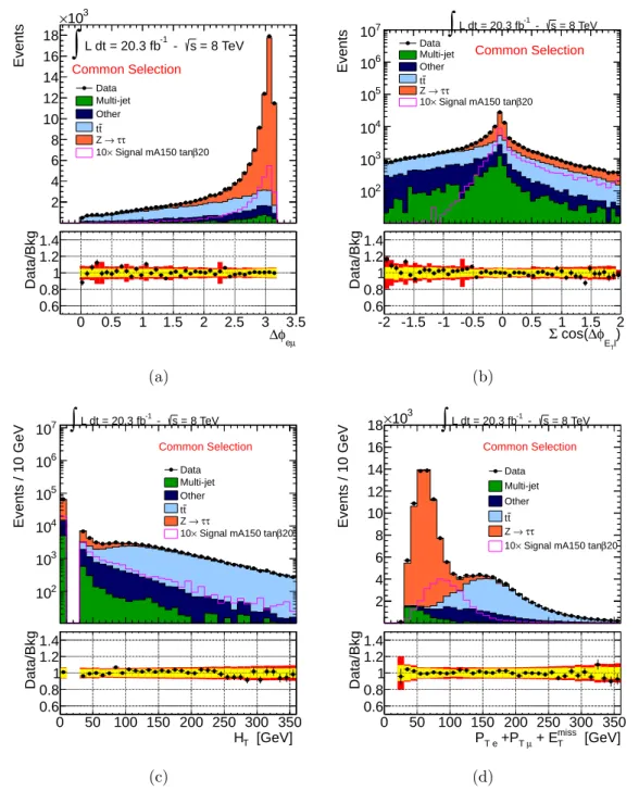
5.2.1. The Common Selection Criteria . . . 61

5.2.2. b-Vetoed Event Category . . . 62

5.2.3. b-Tagged Event Category . . . 63

5.2.4. Mass Reconstruction with the MMC Technique . . . 66

5.3. Background Prediction and Validation . . . 67

5.3.1. Validation of the t ¯ t Background Simulation . . . 70

5.3.2. Measurement of Multi-jet Background . . . 70

5.3.3. Z → τ τ + Jets Background Measurement . . . 76

5.4. Systematic Uncertainties . . . 80

5.4.1. Detector-Related Systematic Uncertainties . . . 80

5.4.2. Theoretical Uncertainties . . . 85

5.4.3. Systematic Uncertainties of Z/γ ^∗ → τ τ Embedded Sample . 86 5.4.4. QCD Multi-Jet Systematic Uncertainties . . . 87

5.5. Results . . . 90

5.5.1. Statistical Interpretation of the Data . . . 90

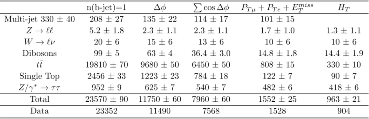
5.5.2. Expected and Observed Events . . . 94

5.5.3. Exclusion Limits on the Signal Production . . . 97

5.5.4. Combination with Other Search Channels . . . 102

Contents

6. Improvements to the MSSM Higgs Boson Search Using Track-

Jets 107

6.1. Track-Based Jets . . . 108

6.2. Performance of the Track-based Jets . . . 110

6.2.1. Track-based Jets Reconstruction . . . 110

6.2.2. B-tagging with Track-Based Jets . . . 112

6.2.3. Use of Track-jets for the MSSM Higgs Boson Search . . . . 116

6.3. Systematic Uncertainties of Track-Jet Reconstruction . . . 118

6.3.1. Material Budget Uncertainty on Track-Based Jets Recon- struction . . . 119

6.3.2. Validation of the Track Subtraction Method . . . 119

6.4. Conclusions . . . 126

7. Summary and Conclusions 127 Acknowledgments 131 Bibliography 133 Appendix A. Additional QCD Studies 145 A.1. Trigger Bias . . . 145

A.2. QCD Additional Plots . . . 147

Appendix B. Additional Plots and Results 149 Appendix C. Further Details on Limit 155 C.1. The ABCD Method . . . 155

C.2. Shape Systematics . . . 156

C.3. Additional Limit Checks . . . 157

C.3.1. Regularization of Signal Samples . . . 163

C.3.2. Pre Fit and Post Fit MMC mass Plots . . . 164

C.3.3. Checks in Mass range 230-300 GeV . . . 167

1. Introduction

The Standard Model (SM) of particle physics describes the strong and electroweak interactions of quarks and leptons and has been confirmed extremely well by exper- iments at energy scales below about 1 TeV. The interactions between the elemen- tary constituents of matter are mediated by gauge bosons based on the principle of local gauge invariance. Masses for all these particles are introduced without spoiling the electroweak gauge symmetry via the mechanism of spontaneous sym- metry breaking. An additional complex scalar field is required for this purpose which give rise to a new scalar particle, the Higgs boson.

The recent discovery at the Large Hadron Collider (LHC) of a new boson of mass of about 125 GeV by the ATLAS and CMS experiments [1,2] is in agreement with the Higgs boson prediction by the SM. The measurements of its properties [3–6] are well compatible with those of the SM Higgs boson. However, the question remains whether this new particle is the only missing piece of the electroweak symmetry breaking sector or whether it is one of several Higgs bosons as predicted by many models beyond the SM. Supersymmetric extension of the SM are theoretically favoured since they offer an elegant solution to limitations of the SM. The minimal supersymmetric extension of the SM (MSSM) predicts the existence of five Higgs bosons, two of them neutral and CP-even (h and H), one neutral and CP-odd (A) and two charged (H ^± ). In this thesis, a search for the neutral MSSM Higgs bosons is performed with 20.3 fb ^{− 1} of proton-proton collision data at a centre-of- mass energy of 8 TeV recorded by the ATLAS experiment at the LHC. Chapter 2 is devoted to an introduction to the MSSM focusing on the Higgs sector and on the neutral MSSM Higgs boson phenomenology.

An overview of the ATLAS experiment is given in Chapter 3. The ATLAS de-

tector consist of four main sub-detectors, the inner detector, the electromagnetic

and hadronic calorimeters and the muon spectrometer. These sub-detectors are

installed cylindrically around the beam pipe in the central barrel part and in disks

in the end-caps which are symmetrical in forward and backward direction with re- spect to the proton beams. The data recorded by the ATLAS experiment undergo several steps of offline reconstruction before being ready for analysis. The physics object reconstruction and data quality criteria used in this thesis are described in Chapter 4.

In Chapter 5, the search for the neutral MSSM Higgs bosons performed in A/h/H → τ ⁺ τ ⁻ → eµ+4ν decays is discussed. This final state corresponds to 6% of the total decay rate of the two τ leptons. In spite of the rather small branching fraction, this final state provides a signal sensitivity which is competitive with the other channels, especially for low Higgs boson masses, because of the high background rejection. The events are split into two mutually exclusive categories based on the presence or absence of b-tagged jets indicating the two main Higgs production modes, in association with b-quarks and via gluon fusion, respectively.

The Higgs boson production in association with b-quarks is characterised by the presence of low transverse momentum b-jets. The reconstruction and calibration of low transverse momenta jets from energy deposits in the calorimeters are strongly deteriorated by pile-up effects of multiple proton interactions per bunch crossing, causing a large loss of efficiency for the A/h/H search in the b-tagged category. As an alternative, jet reconstruction based on inner detector tracks has been studied for the purpose of b-tagging. The inner detector tracks are associated to their original interaction vertex which makes track-based jet reconstruction more robust against pile-up effects than calorimeter-based jets. A study on the prospects for enhancing the sensitivity of the neutral MSSM Higgs boson search by using track- based b-jet identification is presented in Chapter 6.

A summary of the neutral MSSM Higgs boson search and of the prospects for its

improvement by employing track-based jet reconstruction is given in Chapter 7.

2. Higgs Bosons in

Standard Model and MSSM

In this chapter, the theoretical concepts relevant for the experimen-

tal search presented in this thesis are introduced. A brief overview

of the Standard Model of particle physics is given in Section 2.1

based on reference [7]. Among the extensions of the Standard

Model, the minimal supersymmetric extension (MSSM) is theoreti-

cally favoured as one of the most predictive scenarios. The MSSM is

introduced in Section 2.2 with emphasis on the Higgs boson sector

based on references [8,9]. Finally, a review of the phenomenological

aspects of the MSSM Higgs boson production and decays is given

in Section 2.3 based on reference [10].

2.1. The Standard Model of Particle Physics

2.1.1. Introduction

A detailed description of the Standard Model (SM) of particle physics can be found in reference [12]. A brief overview is given below.

The SM of particle physics describes the interactions of the known fermionic mat- ter particles, quarks and leptons, via the strong, the electromagnetic and the weak forces based on the principle of local gauge invariance, i.e. invariance under phase transformations depending on the space-time coordinates. The gravitational force is negligible in atomic and nuclear physics since quantum gravity effects are ex- pected only at very high energies at the Planck scale of ∼ 10 ¹⁹ GeV.

The gauge symmetries of the SM are described by the group SU(3) c ⊗ SU (2) L ⊗ U (1) Y which has 8 + 3 + 1 = 12 generators and gauge fields. The electromagnetic and weak interactions [13–15] are described by the SU (2) _L ⊗ U (1) _Y symmetry group, while SU (3) c is the group of the strong colour forces of Quantum Chro- modynamics (QCD) [16]. A vector boson is associated to each generator of the gauge symmetry groups of the SM acting as mediator of the interaction. Eight gluons are associated to the SU (3) c colour group, while four gauge bosons, W ^± , Z ⁰ and γ, are associated to the electroweak symmetry SU(2) L ⊗ U (1) Y . The gluons and the photon are massless while the remaining weak gauge bosons have mass.

These masses are introduced without spoiling the electroweak gauge symmetry via the mechanism of spontaneous symmetry breaking [17–21], an additional complex scalar field is required for this purpose and give rise to a new scalar particle, the Higgs boson, which interacts with other particles with a strength proportional to their masses.

Quarks are subject to all SM interactions. Each quark flavour is a colour triplet and

carries electroweak charges including electric charges of +2/3 and −1/3 for up-type

and down-type quarks respectively. Leptons are colourless but have electroweak

charges. The electrons, muons and τ leptons carry electric charge −1, while the

associated neutrinos ν _e , ν _µ and ν _τ are electrically neutral. Opposite sign electric

charges are carried by the respective anti-particles. Quarks and leptons group in

three “generations” with equal charge quantum numbers but increasing masses.

2.1. The Standard Model of Particle Physics

2.1.2. The Higgs Mechanism in the SM

The Higgs mechanism extends the Standard Model by a complex scalar field Φ, in its minimal realisation [17–21] one scalar SU (2) L doublet

Φ = φ ⁺

φ ⁰

(2.1) with four degrees of freedom and weak hypercharge Y = +1 is introduced. The Higgs potential

V (Φ) = µ ² Φ ^† Φ + λ(Φ ^† Φ) ² , (2.2) with the mass parameter µ and self coupling λ is invariant under SU(2) L ⊗ U (1) Y

symmetry transformations. For µ ² < 0 the scalar field has an infinite set of degenerate ground states. If a non vanishing vacuum expectation value is chosen for the neutral component of the scalar filed Φ, the SU (2) L ⊗ U (1) Y symmetry is spontaneously broken with the electromagnetic gauge symmetry U(1) _Q remaining as a symmetry of the ground state. Therefore, three of the original four degrees of freedom of the scalar field are absorbed as longitudinal polarisation states of the W ^± and Z bosons, which in this way acquire their masses, while the photon remains massless. The remaining degree of freedom corresponds to a physical massive scalar particle, the Higgs boson.

The masses of the fermions can be generated by means of Yukawa couplings to the Higgs field Φ [22].

2.1.3. Precision Tests and Limitations of the SM

The Standard Model has been successfully tested in a vast number of experiments

over a wide range of energies during the last decades. Precision tests of the elec-

troweak theory performed at LEP, SLC and Tevatron accelerators [25] confirmed

that the couplings of quark and leptons to the weak gauge bosons W ^± and Z fully

agree with the predictions of the SM. Due to the high experimental accuracy of

the per-mille level, not only the tree-level predictions, but also the impact of quan-

tum corrections have been verified. Measurements of weak hadron decays together

with several other experimental results [24] provide additional tests of the Stan-

dard Model at low energies. The recent discovery at the LHC of a Higgs boson

with a mass of about 125 GeV [1, 2] is another success of the SM. The measured

mass is in agreement with the allowed range from the combined measurement of electroweak observables [26]. The spin and coupling strength of the new boson are also in good agreement with the SM predictions for the measured mass.

Tension between the SM predictions and experimental data is found for only very few observables. The most significant discrepancies, of slightly above three stan- dard deviations, are observed for the anomalous magnetic moment of the muon a µ [27] and for the forward-backward asymmetry in bottom quark production at LEP [25] and in the top quark production at the Tevatron [28].

In spite of this success, the Standard Model is conceptually unsatisfactory due to a number of deficiencies and is widely believed to be an effective theory valid only for energies up to the electroweak scale. In addition to the fact that the SM does not include the gravitational force, it does not explain the pattern of fermion masses and, in its simplest version, does not allow for neutrino masses, the theory has other deficiencies indicating the need for new physics beyond the Standard Model (BSM). Some of the most important are discussed below.

Hierarchy and Fine-Tuning Problem The radiative corrections to the Higgs boson mass introduce quadratic divergences in the cut-off energy scale Λ up to which the theory is considered to be valid [29]. If the cut-off scale chosen is the Planck scale or the GUT scale (see below), a fine tuning of the higher order corrections is needed with an unnaturally high precision of O(10 ⁻³⁰ ) to give a Higgs boson mass near the electroweak scale O(100 GeV ) as measured [30–32].

Dark Matter The SM does not contain a particle candidate for the observed large contribution of dark non-barionic matter to the energy density of the Uni- verse [33–35]. Dark matter candidates have to be massive, stable and only weakly interacting particles.

Gauge Unification Problem Another unsatisfactory aspect of the SM is that

the electroweak and strong gauge couplings do not evolve to the same value at

high energies. Motivated by the successful unification of electromagnetic and weak

interaction, the existence of a Grand Unified Theory (GUT) has been suggested [36,

37], which predicts the unification of the three gauge symmetries of the SM in a

2.2. The Minimal Supersymmetric Standard Model

single gauge group with just one coupling constant at the GUT energy scale of about 10 ¹⁶ GeV.

Among many possible extensions of the SM, supersymmetry is theoretically favoured as it provides natural solutions to the above problems. As discussed in Section 2.2, it can solve the hierarchy problem, provide a suitable dark matter particle candi- date and predicts unification of the three SM gauge couplings at the GUT scale.

2.2. The Minimal Supersymmetric Standard Model

2.2.1. Introduction to the MSSM

Supersymmetry (SUSY) [38–40] was first introduced in the 1970s as a new sym- metry relating fermions and bosons. The SUSY generators Q transform fermion fields into boson and vice versa:

Q|Fermioni = |Bosoni, Q|Bosoni = |Fermioni . (2.3) In a supersymmetric extension of the SM, each of the known fundamental particle states is either in a chiral or gauge supermultiplet together with a superpartner with spin differing by unit 1/2.

SUSY naturally solves the hierarchy problem since the quadratically divergent loop contributions to the Higgs mass from SM particles are cancelled by loop contributions from the superpartners. The quark and lepton superpartners are labelled by adding an “s” in front of the name, standing for scalar. The SM gauge bosons also have spin-1/2 partners named by adding “ino” as suffix to the name.

The symbol of superpartners results from adding “(˜)” to the SM symbol. The SUSY particles share the same couplings with their SM partners. Since the left- and right-handed components of fermions shows to transform differently under the weak SU (2) gauge symmetry, their superpartner inherit this feature.

The minimal supersymmetric extension of the Standard Model (MSSM) [41–46],

is defined by requiring the minimal gauge group as in the SM and minimal particle

content: the three generations of fermions (without right-handed neutrinos) and

Table 2.1.: The chiral supermultiplets of the first generation in the minimal su- persymmetric Standard Model (see ref. [8]). The spin-0 fields are complex scalars and the spin-1/2 left-handed two-component Weyl spinors.

Names Supermultiplets Spin 1/2 Spin 0 quarks, squarks Q (u L d L ) (˜ u L d ˜ L )

¯

u u ^† _R u ˜ ^∗ _R

d ¯ d ^† _R d ˜ ^∗ _R leptons, sleptons L (ν e L ) (˜ ν e ˜ L )

¯

e e ^† _R ˜ e ^∗ _R Higgs bosons, Higgsinos H 1 ( ˜ H ₁ ⁰ H ˜ ₁ ⁻ ) (H ₁ ⁰ H ₁ ⁻ )

H 1 ( ˜ H ₂ ⁺ H ˜ ₂ ⁰ ) (H ₂ ⁺ H ₂ ⁰ )

gauge bosons of the SM and two Higgs doublets with their superpartners. The chiral and gauge supermultiplets of the MSSM are listed in Tables 2.1 and 2.2, respectively. The superpartners of the Higgs bosons, the higgsinos, the wino and bino mix with each other resulting in the following mass eigenstates: two charginos χ ^± _1,2 and four neutralinos χ ⁰ _1,2,3,4 .

R-parity conservation

The MSSM requires an additional discrete and multiplicative symmetry called R-parity [40] which ensures the baryon and lepton number conservation. The R-parity quantum number is defined by:

R p = (−1) ^{2s+3B − L} , (2.4)

where L and B are the lepton and baryon numbers and s the spin quantum num-

ber. The R-parity quantum number has a value of +1 for ordinary SM particles

and of −1 for their superpartners. This symmetry was originally introduced as

2.2. The Minimal Supersymmetric Standard Model

Table 2.2.: The gauge supermultiplets in the minimal supersymmetric Standard Model (see ref. [8]).

Names Supermultiplets Spin 1 Spin 1/2 gluons, gluinos G a (a =1,...,8) g g ˜ W bosons, winos W a (a=1,...,3) W ^± , W ⁰ W ˜ ^± , W ˜ ⁰

B boson, bino B B ⁰ B ˜ ⁰

a simple solution to prevent fast proton decay. Lepton and baryon number vio- lation usually leads to proton decays via supersymmetric particle exchange with a life-time shorter than the experimental lower bound. R-parity conservation has also other important phenomenological consequences: SUSY particles are always produced in pairs and decay into an odd number of SUSY particles. Furthermore, the lightest SUSY particle, often chosen to be one of the neutralinos, is stable and therefore is a candidate for the dark matter.

The Soft SUSY Breaking

If supersymmetry is an exact symmetry of nature, the SM particles and their cor-

responding superpartners have the same mass. However, SUSY particles have not

yet been observed, suggesting that these particles, if they exist, must be much

heavier than their SM partners, leading the breaking of supersymmetry at low

energies. To achieve SUSY breaking without reintroducing the quadratic diver-

gences in the Higgs mass radiative corrections, so called “soft” SUSY breaking

terms are introduced in the Lagrangian [47, 48]. These terms introduce explic-

itly the mass terms for the higgsinos, gauginos and sfermions as well as tri-linear

coupling terms between sfermions and higgsinos. In general, if generation mixing

and complex phases are allowed, the soft SUSY breaking terms introduce a large

number of unknown parameters (about 125) [49]. However, in the absence of such

phases and mixing, and by requiring the soft terms to obey certain boundary con-

ditions [47,48], the number of free parameters can be strongly reduced by an order

of magnitude.

2.2.2. The Higgs Sector of the MSSM

In the MSSM, two SU (2) _L doublets of complex scalar fields of opposite hypercharge are required to break the electroweak symmetry. This requirement is necessary to separately generate the masses of up-type and down-type fermions [39, 50, 51] and to cancel chiral anomalies that otherwise would spoil the renormalizability of the theory [52]. The two Higgs doublets are

H 1 = H ₁ ⁰

H ₁ ⁻

with Y H 1 = −1, and H 2 = H ₂ ⁺

H ₂ ⁰

with Y H 2 = +1 . (2.5) The Higgs mechanism in the MSSM [41, 53] is similar to the one in the SM. Non vanishing vacuum expectation values of the neutral components of the two Higgs doublets

hH ₁ ⁰ i = √ v 1

2 , and hH ₂ ⁰ i = √ v 2

2 , (2.6)

break the SU (2) L ⊗ U (1) Y symmetry while preserving the electromagnetic sym- metry U (1) _Q . Three of the original eight degrees of freedom of the scalar fields are absorbed as longitudinal polarization states of the W ^± and Z bosons, which in this way acquire their masses. The remaining degrees of freedom correspond to five physical Higgs bosons: two neutral CP-even bosons h and H, a neutral CP-odd boson A and a pair of charged bosons H ^± .

The MSSM Higgs sector is described by six parameters: the Higgs bosons masses m h , m H , m A , m _H ^± , the mixing angle α of the neutral CP-even Higgs bosons and the ratio between the two vacuum expectation values tan β = v 1 /v 2 . At tree level, only two of these parameters are independent, commonly chosen to be tan β and m A . Supersymmetry imposes a strong hierarchical structure of the Higgs boson mass spectrum: where h is the lightest boson with m h < M Z at three level, while m _A < m _H and M _H ² ± = m ² _A M _W ² . Furthermore, the following relation holds between the mixing angles:

cos ² (β − α) = m ² _h (M _Z ² − m ² _h )

m ² _A (m ² _H − m ² _h ) . (2.7)

These relations are broken by large radiative corrections to the Higgs bosons

masses [54] which raise the upper bound on the h boson mass from M _Z to about

140 GeV. In addition, the requirement of gauge coupling unification restricts tan β

to the range 1 > tan β > m t /m b [55].

2.3. Phenomenology of the Neutral MSSM Higgs Bosons

H i

V µ

V ν

(a)

V µ

H i

H j

(b)

V µ

V ν

H j

H i

(c)

Figure 2.1.: Feynman diagrams for the couplings of (a) one Higgs boson and two gauge boson fields, (b) two Higgs bosons and one gauge boson and (c) two Higgs bosons and two gauge bosons in the MSSM [9].

2.3. Phenomenology of the Neutral MSSM Higgs Bosons

2.3.1. MSSM Higgs Bosons Couplings to SM Particles

The phenomenology of the MSSM Higgs bosons depends on their couplings to the Standard Model and to supersymmetric particles. A short overview of the former is given below based on the ref. [9]. Supersymmetric particles are assumed to be too heavy for direct Higgs bosons decays into them.

The possible couplings between the MSSM Higgs bosons and vector bosons are shown in Figure 2.1. There are the tri-linear couplings V _µ V _ν H _i and V _µ H _i H _j of one Higgs boson and two gauge bosons and of one gauge boson and two Higgs bosons, respectively, as well as quartic couplings V µ V ν H i H j between two Higgs bosons and two gauge bosons. The most relevant coupling for MSSM Higgs boson phenomenology is the tri-linear coupling V µ V ν H i . Since the photon is massless, there are no Higgs-γγ and Higgs-Zγ couplings at tree level. CP-invariance also forbids W W A, ZZA and W ZH ^± couplings. Therefore, for the tri-linear coupling V µ V ν H i only the following terms remain:

Z µ Z ν h ∼ ig z M Z sin(β − α)g µν , Z µ Z ν H ∼ ig z M Z cos(β − α)g µν . (2.8) W _µ ⁺ W _ν ⁻ h ∼ ig w M W sin(β − α)g µν , W _µ ⁺ W _ν ⁻ H ∼ ig w M W cos(β − α)g µν .

(2.9)

The coupling strengths G V V h and G V V H of the neutral CP-even Higgs bosons h and H to a pair of vector bosons are proportional to sin(β − α) and cos(β − α) respectively, where cos(β − α) is given at tree level by equation (2.7). The following relationship holds

G ² _{V V h} + G ² _{V V H} = g _{V V H} ² _SM (2.10) with the SM Higgs boson coupling g V V H SM and has interesting phenomenological consequences. Equations (2.8)-(2.10) imply that the coupling of h (H) to vector bosons increases (decreases) with tan β. For relatively large values ¹ of tan β, h has SM-like couplings to vector bosons while H virtually decouples from them.

An overview of the coupling properties of vector bosons with neutral and charged Higgs bosons, of the tri-linear and quartic couplings among Higgs bosons and of the couplings to SUSY particles is given in [9].

The couplings of the MSSM Higgs bosons to the up-type (u) and down-type (d) fermions also depend on tan β as follows:

G _huu ∝ m u [sin(β − α) + cot β cos(β − α)], G _hdd ∝ m u [sin(β − α) − tan β cos(β − α)] , G _Huu ∝ m _u [cos(β − α) − cot β sin(β − α)], G _Hdd ∝ m _d [cos(β − α) + tan β sin(β − α)] ,

G _Auu ∝ m _u cot β, G _Add ∝ m _d tan β .

The couplings of either the h or H boson to down-type (up-type) fermions is enhanced (suppressed) by a factor tan β depending on the magnitude of cos(β − α) or sin(β − α), while the coupling of the A boson to down-type (up-type) fermions is directly enhanced (suppressed) by tan β.

2.3.2. MSSM Benchmark Scenarios

At tree level, the MSSM Higgs boson masses, decay branching fractions and pro- duction cross sections are all determined by two independent parameters, which by convention are chosen to be m A and tan β. As pointed out in Section 2.2.2, the MSSM Higgs bosons masses are strongly affected by radiative corrections which introduce dependence of physics observables on additional MSSM parameters [54].

The main corrections arise from the top-stop (s)quark sector. For large tan β values, also the bottom-sbottom (s)quark sector becomes increasingly important.

1 For most scenarios this is valid for tan β ? 10 large range of m _A .

2.3. Phenomenology of the Neutral MSSM Higgs Bosons

[GeV]

m A

50 100 150 200 250 300 350 400 [GeV] φ m

50 100 150 200 250 300 350 400

h, Higgs boson H, Higgs boson

mod+

m h

Figure 2.2.: Prediction for the mass of H and h bosons as a function of the mass of the A boson in the m ^mod+ _h scenario with tan β = 10.

Furthermore, the corrections depend on the SUSY-breaking scale M SU SY , the tri- linear Higgs-stop and Higgs-sbottom Yukawa couplings and on the electroweak gaugino and gluino masses.

Due to the large number of free parameters, a complete scan of the MSSM parame- ter space is not practical. To cope with this difficulty, several benchmark scenarios have been proposed [10, 57], which define specific values of the SUSY parameters entering the predictions via radiative corrections and leading to characteristic phe- nomenological features. The parameters m A and tan β are left free and the results are presented in the m A − tan β plane.

The m ^max _h benchmark scenario [56] has been used frequently in the past for neutral MSSM Higgs bosons searches at LEP, Tevatron and the LHC [71–74]. In this scenario, the MSSM parameters are fixed such that the mass m h of the light CP- even Higgs boson assumes its maximum value as a function of m A and tan β. The m ^max _h scenario allows for setting conservative lower bounds on the values of m A , m ^± _H and tan β [57]. However, after the recent discovery of a Higgs boson with mass of about 125 GeV, this scenario predicts a too heavy SM-like Higgs boson h, thus becoming inconsistent with the Higgs boson observation in large regions of the MSSM parameter space. This scenario is now only used for comparison with the result of previous experiments.

Recently, several new benchmark scenarios have been proposed [10] to accom-

modate the experimental constraints from previous searches for neutral MSSM

Higgs bosons and from the observation of a SM-like Higgs boson at the LHC.

An interesting updated benchmark scenario is the m ^mod _h scenario which predicts m h ' 125.5 ± 3 GeV in a large region of the MSSM parameter space, Figure 2.2 shows the prediction for the mass of H and h bosons as a function of the mass of the A boson in the m ^mod _h scenario. The m ^mod _h scenario is obtained by reduc- ing the amount of mixing in the stop sector (between the electroweak eigenstate) with respect to the m ^max _h scenario. This is possible for both signs of the MSSM parameter X t , which determinates the amount of stop mixing, giving rise to two complementary scenarios m ^mod+ _h and m ^mod _h ⁻ . The difference between these two scenarios is found to be negligible for experimental searches and the m ^mod+ _h bench- mark scenario has been used throughout this thesis as a reference. For simplicity, the m ^mod+ _h scenario is referred in the following to as m ^mod _h .

Other interesting benchmark scenarios are the light-stop and the light-stau sce- nario. The first alters the gluon fusion production cross section, while the second leads to a modification of the branching fraction of the decays of the MSSM Higgs boson h into two photons. An overview of the different benchmark scenarios is given in reference [10].

2.3.3. Production and Decay of Neutral MSSM Higgs Bosons at the LHC

The MSSM predicts in large regions of its parameter space a Higgs boson with SM- like couplings. The requirement on this boson to have a mass of about 125 GeV and to be compatible with the previous searches puts stringent constraints on the MSSM parameter space. Scenarios interpreting the discovered SM-like Higgs boson as the lightest CP-even MSSM Higgs boson h are favoured since they have a relatively large region of parameter space still unexplored. This approach is adopted in this thesis.

From the discussion of the Higgs bosons couplings in Section 2.3.1, it turns out that the MSSM Higgs bosons H and A tend to be degenerate in mass and to decouple from gauge bosons. Furthermore their couplings to down-type (up-type) fermions are enhanced (suppressed) proportional to tan β depending on cos(β − α).

Therefore, for large tan β, bottom-quarks and τ-leptons play an important role in

the production and decays of the H and A Higgs bosons compared to the SM

Higgs boson case.

2.3. Phenomenology of the Neutral MSSM Higgs Bosons

g

g b

b

b b

A/h/H τ

τ

(a)

g

b b

b

A/h/H

τ

τ

(b)

q

q g

b

b

A/h/H b

τ

τ

(c)

g

g t/b

A/h/H τ

τ

(d)

Figure 2.3.: Tree-level Feynman diagrams for the production of the neutral MSSM Higgs bosons in association with b-quarks (a,b,c) and via gluon fusion (d) with subsequent Higgs boson decays into a pair of τ leptons.

The production of the neutral CP -even MSSM Higgs bosons h and H at hadron colliders proceeds via the same processes as for the SM Higgs boson production [11].

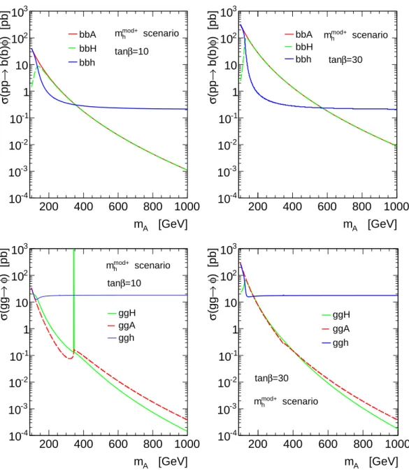
The pseudoscalar boson A, instead, cannot be produced in association with gauge bosons or through vector boson fusion (VBF) at tree-level as the coupling gauge bosons is forbidden by CP -invariance. At the LHC, the dominant neutral MSSM Higgs boson production mechanisms are gluon fusion, gg → A/H/h, and the production in association with b-quarks, pp → b(b)A/h/H. The latter becomes important for relatively large values of tan β (tan β ? 10). Figure 2.3 shows examples of tree-level Feynman diagrams for these processes. The corresponding production cross sections are shown in Figure 2.4 s a function of the A boson mass assuming the m ^max _h benchmark scenario.

The branching fractions for decays of the neutral MSSM Higgs boson h are the same as for the SM Higgs boson (under the assumption that all supersymmet- ric particle are too heavy) while for H and A decays into τ leptons, studied in this thesis, dominate after decays to b ¯ b in large regions of the parameter space.

Figure 2.5 shows the branching fractions for various decays of h, H and A as a

function of m A for two values of tan β in the m ^mod+ _h benchmark scenario.

[GeV]

m A

200 400 600 800 1000

) [pb] φ b(b) → (pp σ

10 -4

10 -3

10 -2

10 -1

1 10 10 2

10 3

bbA bbH bbh

scenario

mod+

m h

β =10 tan

[GeV]

m A

200 400 600 800 1000

) [pb] φ b(b) → (pp σ

10 -4

10 -3

10 -2

10 -1

1 10 10 2

10 3

bbA bbH bbh

scenario

mod+

m h

β =30 tan

[GeV]

m A

200 400 600 800 1000

) [pb] φ → (gg σ

10 -4

10 -3

10 -2

10 -1

1 10 10 2

10 3

ggH ggA ggh

scenario

mod+

m h

β =10 tan

[GeV]

m A

200 400 600 800 1000

) [pb] φ → (gg σ

10 -4

10 -3

10 -2

10 -1

1 10 10 2

10 3

ggH ggA ggh

scenario

mod+

m h

β =30 tan

Figure 2.4.: Predictions of the total cross section for MSSM Higgs bosons produc- tion via gluon fusion and in association with bottom quarks at √

s = 8 TeV using

NNLO calculations and NLO MSTW2008 parton density functions of the proton,

in the m ^mod _h scenario for (left) tan β = 10 and (right) tan β = 30 [11].

2.3. Phenomenology of the Neutral MSSM Higgs Bosons

100 200 300 400 500 600

M

[GeV]

10

10

10

10

10

BR(h)

BR(h -> bb) BR(h -> cc) BR(h -> ττ) BR(h -> µµ) BR(h -> WW) BR(h -> ZZ) BR(h -> γγ) BR(h -> Zγ) BR(h -> gg)

LHC Higgs XS WG 2013

m_h^mod+, tanβ = 10

100 200 300 400 500 600

M

[GeV]

10

10

10

10

10

BR(h)

BR(h -> bb) BR(h -> cc) BR(h -> ττ) BR(h -> µµ) BR(h -> WW) BR(h -> ZZ) BR(h -> γγ) BR(h -> Zγ) BR(h -> gg)

LHC Higgs XS WG 2013

m_h^mod+, tanβ = 50

100 200 300 400 500 600

M

[GeV]

10

10

10

10

10

BR(A)

BR(A -> bb) BR(A -> ττ) BR(A -> µµ)

LHC Higgs XS WG 2013

m_h^mod+, tanβ = 10

100 200 300 400 500 600

M

[GeV]

10

10

10

10

10

BR(A)

BR(A -> bb) BR(A -> ττ) BR(A -> µµ)

LHC Higgs XS WG 2013

m_h^mod+, tanβ = 50

100 200 300 400 500 600

M

[GeV]

10

10

10

10

10

BR(H)

BR(H -> bb) BR(H -> ττ) BR(H -> µµ) BR(H -> WW)

LHC Higgs XS WG 2013

m_h^mod+, tanβ = 10

100 200 300 400 500 600

M

[GeV]

10

10

10

10

10

BR(H)

BR(H -> bb) BR(H -> ττ) BR(H -> µµ) BR(H -> WW)

LHC Higgs XS WG 2013

m_h^mod+, tanβ = 50

Figure 2.5.: Branching fractions of decays of the neutral MSSM Higgs bosons

h/H/A in the m ^mod+ _h scenario for tan β = 10 (left) and tan β = 50 (right) [10].

[GeV]

m A

200 300 400 500 600 700 800 900 1000

β tan

0 1 2 3 4 5 6 7 8 9 10

Preliminary ATLAS

Ldt = 4.6-4.8 fb

∫

= 7 TeV, s

Ldt = 20.3 fb

∫

= 8 TeV, s

b τ , b τ , ZZ*, WW*, γ γ

→ Combined h

d

] κ

u

, κ

V

, κ Simplified MSSM [

Exp. 95% CL Obs. 95% CL

Figure 2.6.: Regions of the m A − tan β plane of a simplified MSSM model [59, 60]

excluded by fits of Higgs couplings (k V and k u,d to vector bosons and up- and down-type fermions, respectively) to the measured Higgs boson production and decays rates. The the observed (shaded) and expected (hashed) exclusions limits at a 95% confidence level [58] are shown.

2.3.4. Status of the Search for Neutral MSSM Higgs Bosons

Constraint of the MSSM Higgs sector may be obtained in two ways: by the measure of the couplings of the observed SM-like Higgs boson to known SM particles or by direct searches for additional Higgs bosons in a well defined scenario.

In case the discovered SM-like Higgs boson with a mass of about 125 GeV is interpreted as the light CP-even Higgs boson of the MSSM, the couplings of the Higgs boson to vector bosons (k V ), up-type fermions (k u ) and down-type fermions (k _d ), can be expressed as a function of m _A and tan β allowing to exclude certain region of the m A −tan β plane [58]. Figure 2.6 shows the excluded parameter region for a so-called “simplified MSSM” model [59,60] obtained from the fits of the Higgs boson production and decay rates to the corresponding observed values.

The latest constraints on m A − tan β plane from direct searches for neutral MSSM

Higgs bosons searches at ATLAS [61] and CMS [73] are shown in Figure 2.7.

2.3. Phenomenology of the Neutral MSSM Higgs Bosons

[GeV]

m A

100 200 300 400 500 600 700 800 9001000

β tan

0 10 20 30 40 50 60

Observed CLs Expected CLs 1 σ 2 σ

1 σ Observed CLs ± theory cross section unc.

τ τ

→ h/H/A

=8 TeV, s

Preliminary, ATLAS

L dt = 19.5 - 20.3 fb -1

∫

>0 µ

max , MSSM m h

= 1 TeV M SUSY

[GeV]

m A

200 400 600 800 1000

β tan

0 10 20 30 40 50 60

scenario

max

MSSM m h

= 1 TeV M SUSY

95% CL Excluded:

observed expected

expected σ

± 1

expected σ

± 2 LEP

at 8 TeV at 7 TeV, 19.7 fb

, 4.9 fb

τ τ

→ CMS Preliminary, H

Figure 2.7.: Expected and observed limits 95% confidence level upper limits on

tan β as a function of m A in the m ^max _h scenario from (top) the ATLAS [61] and

(bottom) CMS [73] experiments.

3. The ATLAS Detector at the LHC

The Large Hadron Collider (LHC) located at the European Organi- sation for Nuclear Research (CERN) in Geneva, Switzerland, is the largest particle collider facility in the world, colliding protons and heavy ions at the so far largest centre-of-mass energies. The ATLAS experiment is one of the experiments at the LHC designed to search for a wide range of new physics phenomena and to perform preci- sion measurements of Standard Model processes. Proton-proton collision data recorded by the ATLAS detector in 2012 has been used for the search for the neutral MSSM Higgs bosons presented in this thesis.

The chapter is organised as follows: the design and performance of

the LHC are summarised in Section 3.1, based on [62], while the

ATLAS detector is described in Section 3.2, based on [63].

3.1. The Large Hadron Collider

The LHC is a hadron synchrotron collider with superconducting magnets. It is installed in the tunnel of the former Large Electron-Positron collider (LEP) with a circumference of about 27 km. LHC is designed to collide proton beams at a centre- of-mass energy of 14 TeV and an unprecedented peak luminosity of 10 ³⁴ cm ^{− 2} s ^{− 1} . It can also collide heavy ion (lead) beams carrying an energy of 2.8 TeV per nucleon at a peak luminosity of 10 ²⁷ cm ^{− 2} s ^{− 1} .

Figure 3.1 shows the layout of the CERN accelerator complex. The protons un- dergo several acceleration steps before injection into the LHC machine. A linear accelerator (Linac 2) brings the protons to an energy of 50 MeV at which they are injected into the Booster where they are further accelerated to 1.4 GeV. The proton energy is successively increased to 25 GeV and to 450 GeV in the Proton Synchrotron (PS) and the Super Proton Synchrotron (SPS), respectively. Finally the protons are injected in two opposite directions into the LHC ring where they reach their final energy.

The proton beams are housed in two separate vacuum pipes and consist of up to 2835 proton bunches, each of them containing about 10 ¹¹ protons. Radiofrequency cavities are employed to accelerate the protons while superconducting magnets bend and focus the beams. The nominal bunch spacing allows for bunch crossings every 25 ns which represents a challenge for the detector read-out electronics.

First proton-proton collisions took place at the LHC in 2009 at a centre-of-mass

energy of 900 GeV followed by collision at 7 TeV in 2010. The LHC successfully

delivered data with increasing instantaneous luminosity during the years 2011 and

2012. The centre-of-mass energy was increased to 8 TeV in 2012. Peak luminosities

of about 4×10 ³³ cm ^{− 2} s ^{− 2} and 8×10 ³³ cm ^{− 2} s ^{− 2} have been reached in years 2011 and

2012, respectively. The physics program of the LHC is carried out by four major

experiments, ATLAS [63], CMS [65], LHCb [66] and ALICE [67]. The ATLAS

experiment recorded proton-proton collision data corresponding to an integrated

luminosity of 4.57 fb ^{− 1} during 2011 and additional 20.3 fb ^{− 1} during 2012. The

data recorded during these two years led to one of the major milestones in particle

physics, the discovery of a Higgs boson with a mass of about 125 GeV.

3.1. The Large Hadron Collider

Figure 3.1.: Illustration of the CERN accelerator complex [64]. The acceleration

of the protons starts in Linac2 followed by the Booster. The Proton Synchrotron

(PS) and the Super Proton Synchrotron (SPS) further accelerate the protons until

their final injection into the LHC, where they acquire their final collision energy.

Figure 3.2.: Cut-away view of the ATLAS detector with its sub-detectors [63].

3.2. The ATLAS Detector

The ATLAS detector is a multi-purpose detector aiming to explore a wide range

of physics phenomena at the Teraelectronvolt energy scale. The physics goals

impose strong requirements on particle reconstruction efficiency and accuracy. A

schematic view of the ATLAS detector is shown in Figure 3.2 . With a length of

44 m and a height of 25 m it is the largest detector at the LHC, it is installed

at one of the LHC interaction points about 100 below ground. ATLAS consists

of four sub-detectors which are installed cylindrically around the beam pipe in

the central barrel part and in disks in the endcap parts which are symmetrically

in the forward and backward direction with respect to the proton beams. The

innermost sub-detector is the inner detector (ID), followed by the electromagnetic

calorimeter, the hadronic calorimeter and finally the muon spectrometer (MS) in

the outermost layer. Each of these sub-detectors is briefly described below based

on reference [63].

3.2. The ATLAS Detector

Figure 3.3.: Cut-away view of the ATLAS inner detector [63].

3.2.1. The ATLAS coordinate system

The right-handed ATLAS coordinate system has its origin at the interaction point.

The z−axis is pointing along the beam direction, the y−axis upwards and the x−axis towards the centre of the LHC ring. The azimuthal angle φ is defined in the transverse plane orthogonal to the beam axis starting from the positive side of the x−axis. The polar angle θ is defined with respect to the z−axis.

A commonly used kinematical variable at collider experiments is the rapidity y = 1/2 · ln

E + p z

E − p z

, (3.1)

where E and p z are the particle energy and the momentum component in z- direction, respectively. The difference in rapidity of two particles is independent of Lorentz boosts along the beam axis. In the limit where the particle veloc- ity approaches the speed of light and for massless particles the rapidity can be approximated by the pseudo rapidity

η = 1/2 · ln θ

2

. (3.2)

The ATLAS detector is divided into the barrel region with cylindrical geometry extending up to |η| > 1.5 (depending on the particular sub-detector) and the endcap regions with a disk structure at larger η values. The angular separation between two particles is commonly measured by ∆R = p

∆η ² + ∆φ ² , where

∆η and ∆φ are the difference in pseudo rapidity and azimuthal angle between the particles, respectively.

3.2.2. The Inner Detector

In the inner detector curved trajectories of charged particles are reconstructed in a 2 T solenoidal magnetic field providing measurements of the particle momenta and of the position of the interaction vertices. The layout of the inner detector is illustrated in Figure 3.3. It has a length of 5.3 m, a diameter of 2.5 m and consists of three independent detector modules with high granularity covering the pseudo rapidity region |η| < 2.5 . The innermost inner detector module is the pixel detector which consists of three cylindrical layers of silicon pixel sensors in the barrel and three disks in the endcap regions. The pixel layer closest to the beam pipe is referred to as B-layer, since it provides crucial informations for the identification of b-quarks. The pixel sensors have a spatial resolution of 10 µm in the transverse and 115 µm in the longitudinal direction with respect to the beam.

The Semi-Conductor Tracker (SCT) surrounds the pixel detector in four cylindrical layers of silicon microstrip sensors in the barrel and nine disks in each of the endcap regions. The spatial resolution of the SCT sensors is 17 µm in the transverse and 590 µm in the longitudinal direction.

The outermost inner detector module is the Transition Radiation Tracker (TRT).

It is composed of 4 mm diameter Kapton straw tubes with a tungsten wire in their centre. The tubes are filled with a gas mixture of 70% Xe, 27% CO 2 and 3%

O 2 which allows for the detection of transition radiation photons. This detector measures the particle position only in the transverse plane.

3.2.3. The Calorimeter System

An illustration of the ATLAS calorimeter system is given in Figure 3.4. It con-

sists of an electromagnetic calorimeter (EM) surrounded by a hadron calorimeter

3.2. The ATLAS Detector

Figure 3.4.: Cut-away view of the ATLAS calorimeter system [63].

which cover the pseudorapidity range |η| < 4.9. Both calorimeters are sampling calorimeters alternating passive absorber plates to active material where the signals are produced. The total detector material at η = 0 corresponds to 9.7 hadronic interaction length λ.

The liquid-argon (LAr) EM calorimeter is ideally suited for precision measurement of electron and photon energies. Liquid argon is used as active material while lead is used as absorber. The EM calorimeter extends up to |η| = 3.2 . The total thickness of the EM calorimeter is about 22 radiation lengths in the barrel and greater than 24 in the end-caps. In the barrel part, it is divided in depth into three cylindrical layers which are segmented into η − φ cells of varying size depending on the layer and on pseudorapidity. The φ cell sizes rage from 0.025 to 0.1, while the η sizes range from 0.0035 to 0.075 . The energy resolutions for electrons and for photons are ranges from 9 − 22%/ √

E and from 8 − 14%/ √

E, respectively, depending on pseudorapidity.

The hadron calorimeter has a coarser granularity than the EM calorimeter and

serves for the reconstruction of hadron jets and the measurement of the missing

transverse energy. It is divided into three sub-detector systems which use differ-

ent technologies to cope with the η-dependent radiation environment. The tile

Figure 3.5.: Cut-away view of the ATLAS muon spectrometer system [63].

calorimeter covers the pseudorapidity range |η| < 1.7 . Scintillating tiles are em- ployed as active material and steel as absorber. In the end-cap regions, a LAr hadron calorimeter (HEC) is used which extends up to |η| = 3.2 and uses Argon as active and copper as absorber material. The forward regions at 3.1 < |η| < 4.9 are instrumented with liquid-Argon Forward CALorimeters (FCAL) which are di- vided into three modules. In the module closest to the interaction point, copper is used as absorber material, while the other two modules employ tungsten. The jet energy resolution in the barrel is about 15% for jets with p T = 50 GeV and about 7% for jets with p T = 1 TeV [117].

3.2.4. The Muon Spectrometer

The muon spectrometer is instrumented with separate high-precision tracking and

muon trigger chambers. The muon momenta are measured by reconstructing the

curvature of the muon trajectory in a toroidal magnetic field of 0.3-1.2 T which

is produced by large superconducting air-core toroid magnets. The layout of the

muon spectrometer is shown in Figure 3.5.

3.2. The ATLAS Detector

Precision measurement of the track coordinates in the bending plane of the mag- netic field is provided by three layers of Monitored Drift Tube (MDT) chambers covering the pseudo rapidity range |η| < 2.7 . Because of the high background rates at large pseudo rapidities, |η| > 2, Cathode Strip Chambers (CSC) are used close to the beam-pipe in the inner end-cap layers. The CSC are multi-wire proportional chambers with cathodes segmented into strips. The muon spectrometer allows for a muon momentum resolution of better than 10% for momenta up to 1 TeV. The best momentum resolution of 3-4% is achieved for muons with transverse momenta of about 100 GeV.

The muon trigger chambers cover the pseudo rapidity range |η| < 2.4 . Resistive Plate Chambers (RPC) are used in the barrel and Thin Gap Chambers (TGC) in the end-cap regions provide a relatively coarse but fast muon momentum mea- surement for the Level-1 muon trigger.

3.2.5. The Trigger System

At a nominal LHC bunch crossing rate of 40 MHz, it is impossible to record and store the data of each bunch crossing. A highly selective trigger system is designed to reduce the initial rate to about 300 Hz keeping the interesting events. The triggering is performed in three stages with increasing sophistication: the Level-1 (L1), the Level 2 (L2) triggers and the event filter (EF). Each trigger level refines the decisions made at the previous level.

The L1 trigger is hardware based and designed to reach a decision within a la- tency of less than 2.5 µs reducing the initial rate to about 75 KHz. It relies on coarse energy measurement in the calorimeters and on muon momenta information provided by the RPC and TGC chambers. It selects high transverse-momentum muons, electrons, photons, jets and τ leptons decaying into hadrons, as well as large missing and total transverse energy. The L1 defines in each triggered event regions of interest (RoI) in η and φ which are further investigated by the higher- level triggers.

The L2 trigger selection is seeded by the RoI information provided by the L1 trigger. Unlike the L1 trigger, the L2 trigger uses the full detector granularity within the RoIs allowing for a more precise reconstruction of particle properties.

The L2 triggers reduce the event rate to approximately 3.5 kHz.

The final stage of the event selection is the event filter which reduces the event rate to 300 Hz. It uses the offline reconstruction algorithms described in Chapter 4 .

3.2.6. Luminosity Measurement

A precise measurement of the recorded instantaneous and integrated luminosity is essential for all physics studies. Several luminosity measurement techniques are employed as described in [69]. The detectors relevant for the luminosity monitoring are the inner detector, the beam conditions monitor (BCM) [69] and the LUCID detector [70]. The inner detector provides a luminosity measurement from the average number of reconstructed proton-proton interactions per bunch crossing. The LUCID detector surrounds the beam pipe on both sides of the interaction point at a distance of 17 m. It consist of Cherenkov detectors which measure the particle flux from the interaction point in very forward direction.

The BCM detector consists of four small diamond sensors arranged around the

beam pipe in a cross pattern on each side of the interaction point. It is a fast

detector primarily designed to monitor the beam condition which also provides an

independent luminosity determination. The overall uncertainty in the luminosity

measurement using these methods is about 3%.

4. Reconstruction of Physics Objects

The raw ATLAS data containing signals of all detector read-out chan-

nels, need to undergo several reconstruction steps before they can be

analyzed. The event reconstruction software is implemented in the AT-

LAS software framework ATHENA [97]. This chapter describes the pro-

cedure for the reconstruction of physics objects relevant for the analysis

presented in this thesis. For a detailed overview of the ATLAS detector

reconstruction software see [98].

4.1. Reconstruction of Charged Particle Tracks

The reconstruction of charged particles tracks and interaction vertices is based on the measurements in the inner detector which allow for the reconstruction of tracks within the pseudorapidity range of |η| < 2.5. A track is characterized by its four-momentum vector and two impact parameters: d 0 , i.e., the distance of closest approach between the track and the interaction point in the transverse plane and z 0 , i.e. the z coordinate of the track calculated at the same point of closest approach.

Tracks are reconstructed by the inner detector track reconstruction software [99].

First raw data from the pixel and SCT detectors are transformed into three- dimensional space points (so called “hits”), while the TRT detector information is translated into drift circles. Subsequently, track seeds are formed from a combina- tion of space-points in the three pixel layers and the first SCT layer. These seeds are then extrapolated through the SCT to form track candidates from all hits on the track path. The track candidates are obtained by a fit trough all hits using a Kalman filter algorithm [100]. Ambiguities in the association of the hits to the track are resolved by this fitting procedure and tracks produced by a random asso- ciation of hits are rejected. The selected tracks are then extrapolated to the TRT and finally refitted using the full information of all three tracking detectors. In order to improve the tracking efficiency for secondary tracks from photon conver- sion or decays of long-lived particles (like kaons), a complementary algorithm [99]

searches for unassociated track segments in the TRT, these segments are then extrapolated towards the SCT and the pixel detector in a similar manner as in the default algorithm. All tracks with p T > 100 MeV are considered for physics analysis.

4.2. Vertex Reconstruction

The vertex reconstruction algorithm and its performance are described in detail

in [98,101] and only briefly summarized here. The vertex finding algorithm selects

a set of well reconstructed tracks and generates a vertex seed according to the

average value of the tracks z coordinate. The z coordinate of the tracks is computed

relative to the expected average position of the collision point. An adaptive vertex

fitting algorithm [102] determines the vertex position based on the vertex seed and

4.3. Electron Reconstruction and Identification

on the tracks around it via a χ ² fit. Based on this fit, tracks that are incompatible with the found vertex by more than seven standard deviations are used to seed the next vertex. The procedure is performed iteratively until either all tracks are associated to a vertex or no additional vertex can be found. The performance of this procedure depends on the expected position of the average interaction point which is monitored during LHC data taking and is computed in intervals of a few minutes as described in [103].

The vertex with the largest sum of transverse momentum of all associated tracks is identified as the primary vertex (PV), corresponding to the interaction point of the hard scattering process in the event. All other vertices in the event are assumed to result from minimum bias interactions and are called pile-up vertices. In data recorded during 2012, there were on average 21 multiple interactions occurring per bunch crossing. Such a high vertex multiplicity strongly affects the ambient energy density in the event, such that an accurate pile-up description in simulation is crucial for the modelling of physics processes. In ATLAS, events are simulated assuming various pile-up conditions and weighted such to reproduce the observed average number of interactions per bunch crossing.

4.3. Electron Reconstruction and Identification

Electron are reconstructed and identified by combining EM calorimeter and in- ner detector measurements. The corresponding dedicated algorithm is described in [104]. The electron candidate is reconstructed as a clusters of EM calorimeter cells which is matched to a track in the inner detector. Special care during the matching is taken to account for Bremsstrahlung losses of the charged particle.

The electron energy is computed as a weighted average between the cluster energy and the track momentum. Several corrections are applied to take into account energy losses in the material of the inner detector and effect of electromagnetic shower leakage. The electron direction is defined by the corresponding track pa- rameters.

Further identification criteria are applied to electron candidates to reduce con-

taminating contribution of photon conversions and hadronic jets. Three differ-

ent identification criteria are provided based on a multi-variate analysis program

(TMVA [105]) and several selection criteria :