ATLAS-CONF-2013-090 17/04/2014
ATLAS NOTE
ATLAS-CONF-2013-090
August 25, 2013 Minor revision: April 16, 2014
Search for charged Higgs bosons in the τ + jets final state with pp collision data recorded at √
s = 8 TeV with the ATLAS experiment
The ATLAS Collaboration
Abstract
The experimental observation of charged Higgs bosons,
H±, which are predicted by many models with an extended Higgs sector, would indicate physics beyond the Standard Model. This note presents the results of a search for charged Higgs bosons in 19.5 fb
−1of proton-proton collision data recorded at
√s=
8 TeV with the ATLAS experiment, using the
τ+jets channel with a hadronically decaying
τlepton in the final state. For light charged Higgs bosons (m
H+ < mtop), the
tt¯
→ H+bWbproduction mode is dominant, while for heavy charged Higgs bosons, associated production of
tH+is dominant. No evidence for a charged Higgs boson is found. For the mass range 90 GeV
< mH+ <160 GeV, 95%
confidence level upper limits on
B(t → H+b) are set in the range 0.24−2.1%, and for the mass range 180 GeV
< mH+ <600 GeV, 95% confidence level upper limits are set on the production cross section of a charged Higgs boson in the range 0.017
−0.9 pb, both with the assumption that
B(H+→τν)=1.
Minor textual correction with respect to the version of August 25, 2013.
c Copyright 2014 CERN for the benefit of the ATLAS Collaboration.
Reproduction of this article or parts of it is allowed as specified in the CC-BY-3.0 license.
1 Introduction
Charged Higgs bosons, H
+and H
−, are predicted by several non-minimal Higgs scenarios [1, 2], such as models containing Higgs triplets [3] and Two-Higgs-Doublet Models (2HDM) [4]. The observation of a charged Higgs boson
1would clearly indicate physics beyond the Standard Model (SM). In a type-II 2HDM, which is the Higgs sector of the Minimal Supersymmetric Standard Model (MSSM) [5], the main production mode at the Large Hadron Collider (LHC) for charged Higgs bosons with masses m
H+smaller than the top quark mass m
top(in the following called light charged Higgs bosons) is through the top quark decay t
→H
+b. For charged Higgs bosons with m
H+ >m
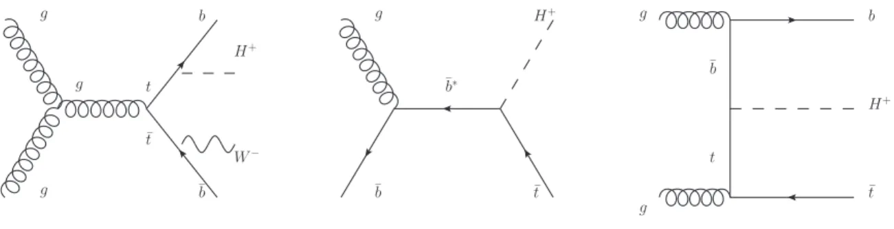
top(called heavy charged Higgs bosons in the following), the main production mode is top quark associated. Feynman diagrams of these processes are shown in Fig. 1. For tan
β >3, where tan
βis the ratio of the vacuum expectation values of the two Higgs doublets, light charged Higgs bosons decay mainly via H
+ →τν[6]; for heavy charged Higgs bosons the branching fraction to
τνcan still be sizeable.
g
g
g t
¯ t
¯b b
H+
W−
H+ g
¯b t¯
g
g
b
H+
¯ t
¯b∗
¯b
t
Figure 1: Example of leading-order Feynman diagrams for the production of charged Higgs bosons at masses below (left) and above (center and right) the top quark mass.
The combined LEP lower limit for the charged Higgs boson mass in a type-II 2HDM with B(H
+→ τν) =1 is m
H+ >94 GeV [7], and the lower limit for any B(H
+ → τν) is 80 GeV. The D0 [8] andCDF [9] collaborations at the Tevatron placed upper limits on B(t
→H
+b) in the 15
−20% range for light charged Higgs bosons. Both the CMS [10] and ATLAS [11, 12] collaborations searched for light charged Higgs bosons assuming B(H
+→τν)=1 and improved the Tevatron limits to the 1
−4% range for a mass range 90 GeV
<m
H+ <160 GeV. The recent discovery of a Higgs boson at the LHC with mass of 125.3
−125.5 GeV and properties resembling those of the SM Higgs boson [13, 14] can be compatible with an extended scalar sector. The new particle can be easily incorporated as one of the scalar particles that are predicted by these theories, e.g. in the MSSM [15].
This note describes the search for a charged Higgs boson produced and decaying as follows:
t¯ t
→[H
+b] [W
−b] ¯
→[(τ
++ντ)b] [q q ¯ b] ¯ (1)
gb ¯
→[¯ t] [H
+]
→[q q ¯ b] [τ ¯
++ντ] (2)
gg→[¯ tb] [H
+]
→[(q q ¯ b)b] [τ ¯
++ντ] (3) where the top quark in Eqs. (2) and (3) decays to a W boson and b quark, and the W boson decays hadronically. The decay products of the W bosons (q, ¯ q) can be observed as jets and the b jets can be identified as such experimentally. In this analysis, only final states with hadronically decaying
τleptons are selected. The visible decay products of the
τlepton (τ
had−vis) can be observed as narrow jets. The neutrinos cannot be detected, leading to missing transverse momentum (E
Tmiss).
1In the following, charged Higgs bosons will be denotedH+, with the charge-conjugateH−always implied.
2 Data and simulated events
This search is performed using data recorded in 2012 by the ATLAS detector at
√s
=8 TeV at the LHC.
The ATLAS detector [16] is a general-purpose particle detector with a cylindrical geometry that consists of several subdetectors surrounding the interaction point and covering almost the full solid angle
2. The trajectory and momenta of charged particles are measured within the pseudorapidity region
|η| <2.5 by multi-layer silicon pixel and strip detectors and a transition radiation tracker. The tracking system is immersed in a superconducting solenoid producing a 2 T axial magnetic field and is surrounded by a high-granularity liquid-argon (LAr) sampling electromagnetic calorimeter with coverage up to
|η|<3.2.
A steel and scintillator tile hadronic calorimeter provides coverage in the range
|η|<1.7. In the forward region LAr calorimeters provide both electromagnetic and hadronic measurements and extend the cover- age to
|η|<4.9. The calorimeters provide good containment for electromagnetic and hadronic showers.
The muon spectrometer surrounds the calorimeters and consists of three large air-core superconducting magnets, each with eight coils, providing an approximately 4 Tm toroidal field, a system of precision tracking chambers, and fast detectors for triggering; it provides coverage up to
|η|<2.7.
Only events recorded with all ATLAS sub-systems operational are used for this analysis. Stringent detector and data quality requirements are applied, including the requirement of having 8 TeV pp colli- sions with stable beams and the availability of the
τhad−vis+E
Tmisstriggers used in this analysis, resulting in a 2012 data sample of 19.5 fb
−1. The uncertainty on the integrated luminosity is 2.8% [17]. It is derived following the same methodology as that detailed in [18], from a preliminary calibration of the luminosity scale derived from beam-separation scans performed in November 2012.
The simulation samples used in this analysis are processed with the ATLAS full GEANT4 simula- tion [19] and are reconstructed using the same analysis chain as the data. Simulated events are overlaid with additional minimum bias events generated with PYTHIA 8 [20] to account for the effect of mul- tiple interactions occurring in the same and neighboring bunch crossings (called pile-up). Prior to the analysis, the simulated events are reweighted to match the distribution of the average number of pile-up interactions in the data.
The event generators are tuned to describe the ATLAS data. In samples where PYTHIA 6 [21] is interfaced to AcerMC [22] the AUET2B [23] tune is used and the PythiaPerugia2011C tune [24] is used if PYTHIA 6 is used with POWHEG [25]. For samples with HERWIG [26], the AUET2 [27] tune is used. In all samples with
τleptons, except for those simulated with PYTHIA 8, TAUOLA [28] is used for the
τdecays, and PHOTOS [29] is used for photon radiation from charged leptons in all samples where applicable.
The background processes that contribute to the search for a charged Higgs boson decaying via H
+ → τνinclude the SM pair production of top quarks (t t ¯
→b bW ¯
+W
−), the production of single top quark events, W boson
+jets, Z boson/γ
∗ +jets, diboson and multi-jet events. The samples of t¯ t and single top quark events are simulated using the generator MC@NLO [30] , except for the t- channel single top quark production, where AcerMC is used. The parton shower and the underlying event simulation are performed with HERWIG and JIMMY [31], respectively, for the MC@NLO samples and with PYTHIA 6 for the AcerMC samples. The top quark mass is set to 172.5 GeV and the CT10 parton distribution function set [32] is used. Inclusive cross sections are taken from the approximate next-to- next-to-leading-order (NNLO) predictions for t t ¯ production [33], for single top quark production in the t-channel and s-channel [34, 35], as well as for Wt production [36]. Overlaps between SM t t ¯ and Wt final states are removed [37]. Single vector boson (W and Z/γ
∗) production with up to five additional
2ATLAS uses a right-handed coordinate system with its origin at the nominal interaction point (IP) in the center of the detector and thez-axis along the beam pipe. Thex-axis points from the IP to the center of the LHC ring, and they-axis points upwards. Cylindrical coordinates (r,φ) are used in the transverse plane,φbeing the azimuthal angle around the beam pipe. The pseudorapidity is defined in terms of the polar angleθasη=−ln tan(θ)/2.
partons is simulated using ALPGEN [38] interfaced to HERWIG and JIMMY, using CTEQ6.L1 [39]
parton distribution functions and cross sections taken from Ref. [40]. Dedicated samples are used with matrix elements for the production of massive c quarks, b b ¯ and c¯ c pairs. Double counting of events with heavy quarks is avoided [41]. Diboson events (WW , WZ and ZZ) are generated with HERWIG. The cross sections are normalized to NNLO predictions for single vector boson production and to next-to- leading-order (NLO) predictions for diboson production [42]. No simulation samples of gluon-initiated multi-jet events are used because of very small selection efficiencies and only limited statistical precision of the samples available. Furthermore, these processes are generally not well-described in simulation.
For 90 GeV
<m
H+ <160 GeV, PYTHIA 6 is used to produce events in the signal processes t t ¯
→b bH ¯
+W
−, t¯ t
→b bH ¯
−W
+and t¯ t
→b bH ¯
+H
−, where the charged Higgs bosons decay as H
+ → τν.W bosons coming from top quarks are allowed to decay inclusively. For 180 GeV
<m
H+ <600 GeV, the signal simulation for top quark associated H
+production is performed with PYTHIA 8 interfaced to POWHEG. The production cross section for the heavy charged Higgs boson is computed using the four- flavor and five-flavor schemes, including theoretical uncertainties, and combined according to Ref. [43].
The samples are generated with the width of the charged Higgs boson much smaller than the detector resolution.
3 Object reconstruction
3.1 Data quality
Basic data quality checks are performed by discarding events where any jet with p
T >25 GeV fails the quality cuts discussed in Ref. [44]. This ensures that no jet in the event is consistent with having originated from instrumental effects, such as large noise signals in the hadronic end-cap calorimeter, coherent noise in the electromagnetic calorimeter, or non-collision backgrounds. In addition, events are discarded if the primary vertex
3has less than five associated tracks.
3.2 Jets
Jets are reconstructed from topological clusters in the calorimeter using the anti-k
talgorithm [45, 46], with a size parameter value R
=0.4. They have a local calibration [47] and correction factors derived from simulation are applied. The local calibration method classifies calorimeter clusters as either elec- tromagnetic or hadronic by considering properties such as the energy density of the cluster, isolation and depth in the calorimeter. Corrections based on jet areas [48] are applied to reduce the effects of pile-up on the jet calibration [49]. Only jets with p
T >25 GeV and
|η|<2.5 are considered.
Additional suppression of the effects of pile-up on jets is achieved through the use of tracking and vertexing information to select jets originating from the hard-scatter interaction. By combining tracks and their vertices with calorimeter jets, a discriminant that measures the probability that a jet originated from a particular vertex can be defined, the Jet Vertex Fraction (JVF) [49]. It is given by the sum of the transverse momenta of tracks that are matched to a jet and originate in the primary vertex divided by the total transverse momenta of all tracks in that jet. If no tracks are matched to a jet, a JVF value of
−1 isassigned. If p
T <50 GeV and
|η|<2.4,
|JVF|>0.5 is required.
A dedicated algorithm combining impact-parameter information with the explicit determination of an inclusive secondary vertex is used to identify jets initiated by b quarks [50]. A working point corre- sponding to an average efficiency of about 70% for b jets in t¯ t events is chosen. Jets tagged as b jets are required to pass the same p
T,
ηand JVF selection as imposed for the nominal jet selection.
3The vertex with the largest sum of trackp2Tin the event is defined as the primary vertex.
3.3 τs
Hadronic decays of
τleptons are characterized by the presence of one or three charged tracks, accompa- nied by a neutrino and possibly neutral pions. This results in a collimated shower profile in the calorime- ter and only a few nearby tracks. Before the object selection and identification, candidates for hadronic
τlepton decays are seeded by jets. In order to reconstruct hadronically decaying
τleptons [51, 52], all anti-k
tjets depositing at least p
T>10 GeV in the calorimeter are considered as
τcandidates. Dedicated algorithms are used in order to reject electrons and muons. Hadronic
τdecays are separated from jets based on the output of a boosted decision tree algorithm. This analysis uses the “tight”
τidentification selection point, yielding an efficiency of about 40% for a
τcandidate with p
T >20 GeV in Z
→ττevents and a rejection factor of about 100− 1000 for quark- and gluon-initiated jets. Only candidates with one or three associated tracks reconstructed in the inner detector are considered. The hadronic decay products of the
τare required to have a visible transverse momentum (p
τT) of at least 20 GeV and to be within
|η|<
2.3.
3.4 Electrons
Since there are no electrons in the final states searched for in this analysis, events containing recon- structed and identified isolated electrons are vetoed. Electron reconstruction begins with tracks in the inner detector that are matched to clustered energy deposits in the electromagnetic calorimeter [53].
Electron candidates are required to pass a “tight” identification selection point, have E
T >25 GeV, and to be in the fiducial volume of the detector,
|η|<2.47. The transition region between the barrel and end- cap calorimeters (1.37
< |η| <1.52) is excluded. Electron candidates must fulfill quality requirements based on the expected shower shape [54]. In addition, the distance of closest approach to the primary vertex along the beam axis,
|z0|, has to be less than 2 mm. Isolation criteria that areE
T- and
η-dependentare imposed in a cone of a radius
4∆R=0.2 (0.3) for calorimeter (tracking) isolation around the electron position, excluding the electron object itself.
3.5 Muons
Events containing reconstructed and identified isolated muons are also vetoed in this analysis. Objects are considered as muon candidates if an inner detector track matches a track reconstructed in the muon spectrometer [55, 56]. Muon candidates are required to have p
T >25 GeV,
|η| <2.5 and
|z0| <2 mm.
Only isolated muons are accepted by passing a mini-isolation algorithm [57] in which the isolation cone around a muon shrinks with increasing muon p
T(maximum
∆R =0.4). The scalar sum of the p
Tof tracks inside that cone, excluding the muon track itself, must be less than 5% of the p
Tof the muon.
When a muon candidate shares the same inner detector track as a selected electron, the full event is discarded.
3.6 Removal of objects with geometric overlaps
ATLAS reconstruction can assign each energy deposit to more than one object. The following removal procedure for overlapping objects is applied in this order before any selected objects are vetoed:
•
Any electrons within
∆R <0.4 of jets passing the nominal p
T,
η, and JVF requirements areremoved.
4∆R ≡ p
(∆η)2+(∆φ)2, where ∆ηis the difference in pseudorapidity of the two objects in questions, and∆φ is the difference between their azimuthal angles.
•
Muon candidates are rejected if they are found within
∆R<0.4 of any jet that passes the nominal p
T,
η, and JVF requirements.•
A
τcandidate is rejected when it is found within
∆R<0.2 of a selected muon or electron.
•
Finally, a jet is removed if found within
∆R<0.2 of a selected
τobject.
3.7 Missing transverse momentum
The missing transverse momentum (E
missT) definition used in this analysis is an object-based defini- tion [58]. It is computed using fully calibrated and reconstructed physics objects.
4 Event selection
The triggers used for this search require a threshold on the transverse momentum of the
τobject of p
τT >29 GeV or
>27 GeV and a requirement that E
missT >40 GeV or
>50 GeV. The
τhad−vis+E
missTtrigger definition varied slightly during the 2012 data-taking period as trigger object thresholds were adjusted to maintain a high efficiency without exceeding the bandwidth of the trigger system while the luminosity increased.
The following requirements are then applied to select events compatible with the signal hypothesis:
•
at least 4 (3) jets pass the p
T,
ηand JVF criteria as described in Sec. 3.2 for the light (heavy) signal selection,
•
at least one of the selected jets must be b-tagged,
•
exactly one hadronically decaying
τhas p
T >40 GeV (this
τhad−viscandidate must match to the
τobject used in the trigger decision),
•
there must be no additional hadronically decaying
τleptons with p
T >20 GeV, nor any muon or electron with p
T>25 GeV,
•
E
missT >65 (80) GeV for the light (heavy) charged Higgs boson search,•
a requirement is placed on the quantity
ETmiss0.5·√P
pPV trkT >13 (12) GeV1/2
in the light (heavy) H
+search. Here p
PV trkTis the transverse momentum of a track originating from the primary vertex and the sum is taken over all tracks from the PV.
The final discriminating variable is the
τhad−vis+E
Tmisstransverse mass, defined as m
T =q
2p
τTE
Tmiss(1
−cos
∆φτ,miss), (4)
where
∆φτ,missis the azimuthal angle between the hadronic decay products of the
τlepton and the di- rection of the missing transverse momentum. In the case of backgrounds that produce a real W boson decaying to (τ
+ν) with a subsequent hadronicτdecay, m
Tcorresponds to the transverse W boson mass.
For the signal hypothesis it corresponds to the transverse H
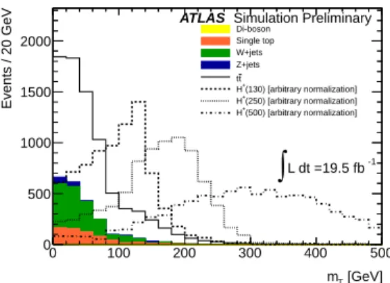
+boson mass. The simulated m
Tdistributions of the dominant SM backgrounds are shown in Fig. 2, overlaid with mass distributions for several signal mass points. Backgrounds are scaled to luminosity while signals are scaled arbitrarily for shape compar- ison. Signal selection efficiencies, including
ηand p
Tcuts on selected objects are given in Table 1 for various H
+mass points.
The m
Tdistribution in data is modeled using a combination of background components and a hypo-
thetical signal component. The background components are described below. The hypothetical signal
component is modeled using simulation across a range of charged Higgs boson masses.
[GeV]
mT
0 100 200 300 400 500
Events / 20 GeV
0 500 1000 1500 2000
Di-boson Single top W+jets Z+jets
t t
(130) [arbitrary normalization]
H+
(250) [arbitrary normalization]
H+
(500) [arbitrary normalization]
H+
L dt = 19.5 fb-1
∫
ATLAS Simulation Preliminary
Figure 2: The transverse mass,
mT, shown for events passing the heavy
H+signal selection. Background contributions from
t¯t, single top quark, single boson and diboson events estimated from simulation areshown stacked while hypothetical signal distributions for different charged Higgs boson masses are over- laid, scaled arbitrarily for shape comparison.
mH+[GeV] 90 100 110 120 130 140 150 160
Efficiency (%) 0.72 0.76 0.85 0.92 1.02 1.19 1.19 1.18
mH+[GeV] 180 190 200 225 250 275 300 350
Efficiency (%) 1.78 1.88 2.00 2.31 2.75 2.93 3.15 3.60
mH+[GeV] 400 450 500 550 600
Efficiency (%) 4.05 4.19 4.48 4.78 4.89
Table 1: The signal selection efficiency, as determined from simulation, as a function of the charged Higgs boson mass.
5 Background modeling
Backgrounds to the search for charged Higgs bosons in the
τ+jets final state can be categorized accord- ing to the origin of the hadronically decaying
τcandidate in the event. For the cases where an electron, muon, or true
τis reconstructed as the
τcandidate of the event, the background prediction is taken from simulated events. The background contribution from events with a correctly identified
τis modified by scale factors that correct the efficiency of the
τhad−visidentification algorithm in simulation to that mea- sured in data [51]. The background contribution with a
τcandidate reconstructed from an electron or muon is suppressed by dedicated lepton veto algorithms. Scale factors are also applied to correct the simulated efficiency of the electron veto algorithm to that measured in data [51].
The final source of background is from events where a jet is misidentified as the
τcandidate of the event. This background arises from both gluon-initiated and quark-initiated jets, and it is assessed using a data-driven method that applies weights calculated from identification and misidentification efficiencies to data events.
The weights for this method are determined based on several relations. First, “loose” and “tight”
τcandidate selections are defined. The loose selection requires the
τhad−visobject selection and trigger- matching, with no requirement on the
τhad−visidentification. The tight
τcandidate selection requires the object to pass both the loose selection and the nominal
τhad−visidentification criteria.
The collections of loose and tight
τcandidates contain both real and misidentified objects, so the total number of events with a single loose or tight
τcandidate can be expressed as:
N
L=N
mL+N
rL; (5)
N
T =N
mT +N
rT,(6) where N
mrefers to the number of misidentified
τcandidates in each case and N
rrefers to the number of real
τs. The superscriptsL and T refer to loose and tight
τcandidates, respectively. Two probabilities are also defined: the probability for a real
τpassing the loose criteria to also pass the tight criteria (p
r), and the probability for a misidentified
τcandidate passing the loose criteria to also pass the tight criteria ( p
m). These can be defined as:
p
m=N
mT/NmL; (7)
p
r=N
rT/NrL.(8)
Using these two sets of equations, one can solve for the total number of misidentified tight
τcandidates as a function of p
r, p
m, and the total numbers of loose and tight
τcandidates, as follows:
N
mT =p
m( p
r−p
m) ( p
rN
L−N
T). (9)
From this equation, one can extract weights to be applied to loose and tight
τcandidates as a function of p
mand p
r. These weights are applied to signal region data events with loose and tight
τcandidates, in order to predict the total background contribution from events with misidentified
τcandidates that pass the tight selection. Specifically, weights are applied to events with tau candidates that either pass only the loose (w
L), or both the loose and tight requirements (w
LT). The weights are defined for these two cases respectively as:
wL=
p
mp
r( p
r−p
m) ; (10)
wLT=
p
m( p
r−1)
( p
r−p
m)
.(11)
The probability p
ris determined using truth-matched hadronically decaying
τs in simulatedt t ¯ events.
The baseline
τhad−vis+E
missTtriggers are required, but without any additional event selection. Systematic uncertainties associated with the simulated true
τare taken into account, and the dominant uncertainty arises from the data-driven calibration of the
τhad−visidentification efficiency [51].
The probability p
mis measured in a W boson
+jets control region where the loose
τcandidate composition is dominated by light quark jets. Events in this control region are triggered by a combined trigger requiring an electron or a muon in addition to a
τcandidate. For the case with an electron, the trigger threshold on the electron p
Tis 18 GeV, and for the case with a muon, it is 15 GeV. For both triggers, the
τhad−vistrigger has a p
Tthreshold of 20 GeV. The control region is further defined using the same event cleaning cuts as the baseline selection, and then requiring:
•
exactly one muon or electron,
•
zero b-tagged jets,
•
at least one loose
τcandidate,
•
m
T(lepton, E
missT)
>50 GeV.
The contamination from correctly reconstructed
τcandidates (7%) and electrons or muons (5%) mis- reconstructed as
τcandidates is subtracted using simulation.
A region dominated by multi-jet events is also used to measure p
m, in order to define the uncertainty
in p
mthat arises from differences in jet composition between regions. This multi-jet region is defined
by the heavy H
+signal region selection with reversed b-tag and E
missTrequirements. Thus, this region
is selected by requiring zero b-tagged jets and E
missT <80 GeV. The difference between this region and
the W boson
+jets region is used to estimate systematic uncertainties on p
mdue to differences in jet
composition (i.e. the relative contributions of quarks and gluons). The use of p
mmeasured from the W boson
+jets region is observed to perform better in the early signal region (before the E
Tmissselection), than the use of p
mmeasured from the multi-jet region. Furthermore, the jet composition of the W boson
+jets region is expected to have a greater similarity than that of the multi-jet region to the jet composition of the signal region. Therefore, the probability p
mmeasured in the W boson
+jets region is chosen as the nominal value for p
m, while the probability measured in the multi-jet region is used to define the systematic.
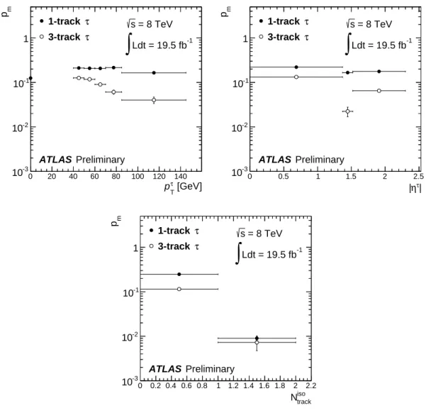
The probabilities p
mand p
rare binned in several properties of the hadronically decaying
τcandidate of the event: the number of associated tracks, the number of tracks in the
τcandidate isolation cone, defined as
∆Rbetween 0.2 and 0.4 from the center of the
τhad−vis(N
trackiso), and the p
τTand
|η|of the
τcandidate (|η
τ|). The values forp
mmeasured in the W boson
+jets region are shown in Fig. 3.
[GeV]
τ
pT
0 20 40 60 80 100 120 140
mp
10-3
10-2
10-1
1
τ 1-track
τ 3-track
ATLAS Preliminary
Ldt = 19.5 fb-1
∫
= 8 TeV s
τ| η
|
0 0.5 1 1.5 2 2.5
mp
10-3
10-2
10-1
1
τ 1-track
τ 3-track
ATLAS Preliminary
Ldt = 19.5 fb-1
∫
= 8 TeV s
iso track
N
0 0.2 0.4 0.6 0.8 1 1.2 1.4 1.6 1.8 2 2.2
mp
10-3
10-2
10-1
1
τ 1-track
τ 3-track
ATLAS Preliminary
Ldt = 19.5 fb-1
∫
= 8 TeV s
Figure 3:
pmmeasured in the
Wboson
+jets control region in data, as a function of
pτT,
|ητ|, andNtrackiso, shown separately for 1-track and 3-track hadronically decaying
τcandidates.
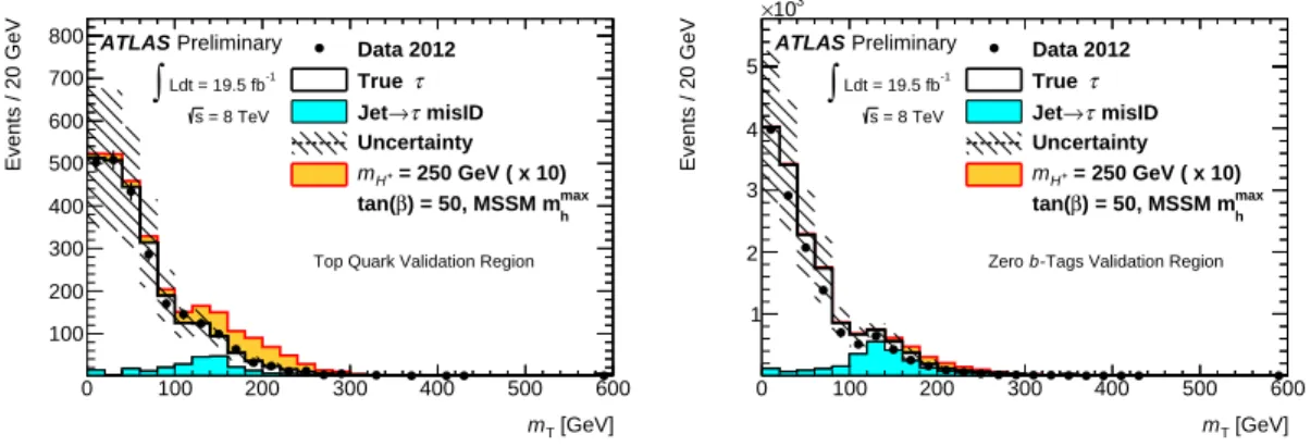
The background modeling is tested using an independent validation region (Fig. 4, left), which is defined by the heavy H
+signal selection, but with exactly 2 b-tagged jets (“top quark validation region”).
In addition, the method is tested in a second independent validation region (Fig. 4, right), defined by
applying the selection criteria for the heavy H
+search, except requiring exactly zero b-tagged jets (“zero
b-tags validation region”). The peak structure seen in the background with jets misidentified as
τhad−visis a result of the kinematic cuts of the event selection, from the relationship between p
τT, E
Tmiss, and the angle between the two in the calculation of m
T. A simulated signal distribution with m
H+ =250 GeV is added in Fig. 4. The cross section is calculated in the m
maxhscenario of the MSSM [59] with the Higgsino mass parameter
µ=200 GeV for tan
β=50 and scaled by a factor of 10 for better visibility.
In the top quark validation region, the background is dominated by t t ¯ events, in both the true
τand jet
→τhad−viscontributions. In the zero b-tags validation region the true
τbackground is dominated by W boson
+jets events and the jet
→τhad−visbackground is dominated by multi-jet events.
[GeV]
mT
0 100 200 300 400 500 600
Events / 20 GeV
100 200 300 400 500 600 700 800
Top Quark Validation Region Data 2012
τ True
misID
→τ Jet Uncertainty
= 250 GeV ( x 10)
H+
m
max
) = 50, MSSM mh
β tan(
Ldt = 19.5 fb-1
∫
= 8 TeV s ATLAS Preliminary
[GeV]
mT
0 100 200 300 400 500 600
Events / 20 GeV
1 2 3 4 5
103
×
-Tags Validation Region b
Zero Data 2012
τ True
misID
→τ Jet Uncertainty
= 250 GeV ( x 10)
H+
m
max
) = 50, MSSM mh
β tan(
Ldt = 19.5 fb-1
∫
= 8 TeV s ATLAS Preliminary
Figure 4: The transverse mass,
mT(τ
had−vis,EmissT), in the top quark validation region (left), and the zero
b-tags validation region (right). All systematic uncertainties are included in the uncertainty band. Asignal contribution with a charged Higgs boson mass of 250 GeV and the MSSM
mmaxhscenario [59]
cross section at tan
β=50 is also shown, scaled up by a factor of 10.
The predicted contribution from events with a jet misidentified as a hadronically decaying
τfor the light and heavy charged Higgs boson searches are shown in Table 2, along with the predictions of backgrounds from other sources and the observed events in data. The systematic uncertainties shown in the table for each source of background are described in Section 6, and the systematic uncertainties of the jet
→τhad−visbackground are specifically described in Section 6.3. As shown in the table, the E
missTselection dramatically reduces the contribution of the fake
τhad−visbackground to the final signal regions.
Cut Jet→τhad−vis Trueτ Lepton→τhad−vis SM (Total) Data
LightH±Selection
Lepton veto 21000±100±4000 14000±200±2000 210±30±30 35000±200±4000 35693 EmissT selection 1300±40±200 7900±200±1400 60±10±20 9300±200±1400 8296 b-tagging 500±30±100 4000±80±800 40±4±10 4500±100±800 4230
HeavyH±Selection
Lepton veto 67000±200±13000 32000±300±4000 500±40±100 100000±400±14000 103953 EmissT selection 3500±60±700 20000±300±3000 180±20±50 24000±300±3000 21280 b-tagging 1000±40±200 7400±100±1400 80±10±20 8500±100±1400 7950
Table 2: Predicted and observed number of events at several points in the light and heavy charged Higgs
boson selections. Statistical uncertainties are shown, followed by systematic uncertainties.
Variation Shift up (%) Shift down (%) Shift up (%) Shift down (%) LightH+event selection HeavyH+event selection
bjet (mis-)tag efficiency uncertainty 3.1 -3.4 2.9 -3.2
Jet energy scale uncertainties 3.7 -4.8 7.1 -6.8
JVF uncertainty 2.2 -1.9 2.2 -2.1
EmissT uncertainties 0.4 0.3 -0.6 -0.2
τhad−vise-veto uncertainty 0.02 -0.02 0.01 -0.01
τhad−visenergy scale uncertainty 3.6 -3.8 3.6 -3.8
τhad−visidentification uncertainty 3.8 -3.8 3.7 -3.7
Pile-up uncertainties 0.9 -1.5 2.6 -2.1
Table 3: The effect of each systematic uncertainty on the final event yield in events passing the light (left) and heavy (right)
H+event selection, respectively. Effects are evaluated for background contributions estimated from simulation. Groups of related systematics are shown here added in quadrature, though they are treated as individual nuisance parameters in the statistical interpretation.
6 Systematic uncertainties
6.1 Systematic uncertainties arising from detector simulation
To assess the impact of systematic uncertainties arising from detector simulation, the selection cuts are re-applied after shifting a particular parameter up and down by one unit of uncertainty. The systematic uncertainties on background contributions containing true hadronically decaying
τs and electrons ormuons misidentified as
τhad−visare evaluated using simulation. The dominant uncertainties arise from the jet and
τhad−visenergy scales, the uncertainty on the b-tagging (mis-)identification efficiency and the
τhad−visidentification uncertainty. More details are given in Table 3. The luminosity uncertainty of 2.8%
is an additional systematic uncertainty on the normalization.
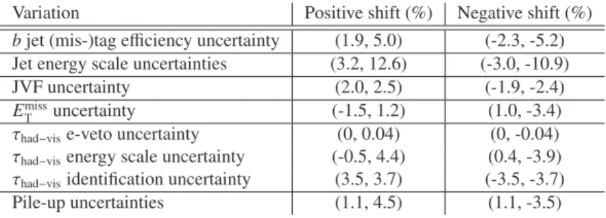
The effects of detector-related systematic uncertainties on the signal samples are shown in Table 4, where the ranges given are the largest and smallest up and down variations for the full range of H
+boson masses, 90
−160 GeV and 180− 600 GeV. For distributions and tables, groups of systematic uncertainties are shown added in quadrature, though they are treated individually in the statistical interpretation of the analysis results.
6.2 Systematic uncertainties arising from the event generation and theoretical t t ¯ cross section
Additional uncertainties are taken into account for the t t ¯ background and H
+signal simulation, as well as the theoretical t t ¯ cross section. All these uncertainties are shown in Table 5.
Systematic uncertainties on the t¯ t generation, which include modeling of parton showers, hadroniza- tion, and the underlying event, are evaluated by computing the acceptance for t t ¯ events produced with MC@NLO interfaced to HERWIG/JIMMY and comparing to events produced with POWHEG inter- faced to PYTHIA 6. There is also an uncertainty on the theoretical t¯ t cross section, which includes both the scale and parton distribution function (PDF) uncertainties.
Since no alternative generator is available for the light H
+signal simulation, an uncertainty on the generator model for the light H
+signal is evaluated using simulated SM t¯ t samples. The generator mod- eling uncertainties for the heavy H
+samples are estimated from a comparison between events produced with MC@NLO interfaced to HERWIGPP, and POWHEG interfaced with PYTHIA 8.
The systematic uncertainties arising from initial and final state radiation (jet production rate) are
computed using t t ¯ samples generated with AcerMC interfaced to PYTHIA 6, where initial and final state
radiation parameters are set to a range of values not excluded by the experimental data [60].
Variation Positive shift (%) Negative shift (%) bjet (mis-)tag efficiency uncertainty (1.9, 5.0) (-2.3, -5.2) Jet energy scale uncertainties (3.2, 12.6) (-3.0, -10.9)
JVF uncertainty (2.0, 2.5) (-1.9, -2.4)
EmissT uncertainty (-1.5, 1.2) (1.0, -3.4)
τhad−vise-veto uncertainty (0, 0.04) (0, -0.04)
τhad−visenergy scale uncertainty (-0.5, 4.4) (0.4, -3.9)
τhad−visidentification uncertainty (3.5, 3.7) (-3.5, -3.7)
Pile-up uncertainties (1.1, 4.5) (1.1, -3.5)
Table 4: The effect of each systematic uncertainty on the final event yield in
H+ →τνevents. For each uncertainty a range of yield shifts is given, indicating the smallest and largest shifts in
mH+ =90
−160 and 180
−600 GeV. Groups of related systematics are shown here added in quadrature, though they are treated as individual nuisance parameters in the statistical interpretation.
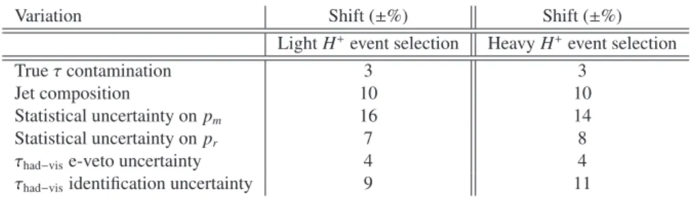
6.3 Systematic uncertainties arising from data-driven background estimation
For the background contributions that are estimated in a data-driven way, systematic uncertainties are listed in Table 6. The largest systematic uncertainty arises from the statistical uncertainty on the mea- surement of p
m. To evaluate this systematic uncertainty, p
mis shifted up and down by one standard deviation, and the weights calculated from these shifted values of p
mare propagated through the back- ground prediction method. The statistical uncertainty on p
r, which is uncorrelated with that of p
m, is treated in a similar fashion.
Other dominant systematic uncertainties arise from the
τhad−visidentification uncertainty and the uncertainty on the jet composition for fake
τcandidates. The first corresponds to the uncertainty on the simulated efficiency of the
τhad−visidentification, which is used for the computation of p
r. The second corresponds to the possible difference in jet composition between the data region where p
mis measured, and the signal region where it is applied. This uncertainty is calculated by taking the difference between the estimate of the background that arises from using the probability p
mmeasured in the W boson
+jets region and that measured in the multi-jet region.
Finally, smaller uncertainties arise from the uncertainty on the subtraction of simulated true leptons (e,
µ,τ) from the region wherep
mis measured. These are dominated by the uncertainties on the efficiency scale factors of the
τhad−visidentification algorithm and the electron veto algorithm.
Source of uncertainty Normalization uncertainty LightH±
Generator model (bbW¯ ±H±) 9%
Generator model (bbW¯ +W−) 9%
t¯tcross section uncertainty 10%
Jet production rate (SM andH±) 11%
HeavyH±
Generator model (H±) 2−9%
Generator model (SM) 8%
tt¯cross section uncertainty 10%
Jet production rate (H±) 4.4−11%
Jet production rate (SM) 11%
Table 5: Systematic uncertainties arising from
tt¯ generator modeling, and from the jet production rate.
The uncertainties are shown for the
t¯tbackground and the charged Higgs boson signal, for the light and
heavy charged Higgs boson selections.
Variation Shift (±%) Shift (±%) LightH+event selection HeavyH+event selection
Trueτcontamination 3 3
Jet composition 10 10
Statistical uncertainty onpm 16 14
Statistical uncertainty onpr 7 8
τhad−vise-veto uncertainty 4 4
τhad−visidentification uncertainty 9 11
Table 6: Systematic uncertainties on the data-driven jet
→τhad−visbackground estimation. The numbers represent symmetric relative shifts in the yields of events with jets misidentified as
τhad−vis, for the light (left) and heavy (right)
H+event selection.
6.4 τ
had−vis+ E
missTtrigger uncertainties
Another major source of uncertainty in the analysis arises from the difference in the
τhad−vis+E
missTtrigger efficiencies in data and simulation. Scale factors for the
τhad−vis+E
missTtrigger efficiencies, which are applied to simulated events, are derived from measuring the efficiency of the
τhad−vis+E
missTtriggers in a muon-triggered region in data and simulation. Events used for these efficiency measurements must:
•
pass the standard event cleaning criteria,
•
pass a muon trigger,
•
contain a muon with p
T>65 GeV,
•
contain at least two jets,
•
contain an identified
τhad−vis,
•
contain at least one b-tagged jet.
The events that pass this selection are dominated by t t ¯
→ µτ+b b ¯
+E
missT, with small contributions from other backgrounds. The requirement of a muon with p
T >65 GeV has been optimized to ensure the closest possible agreement between the E
Tmissdistribution shape of this region and the signal region.
Scale factors are taken from the ratio of the efficiency measured in data to that measured in simulation, in six bins of p
τTand E
Tmiss. These scale factors are shown in Table 7, with statistical uncertainties followed by systematic uncertainties. The total systematic uncertainties in Table 7 are shown added in quadrature, though they are considered separately in the analysis.
Sources of uncertainties on these scale factors arise from the statistical uncertainty of the factors; a potential kinematic bias, evaluated by varying the muon p
Tselection criterion; the effect of binning in number of tracks associated with the
τhad−vis; the effect of binning in trigger periods; and the impact of non-τ backgrounds in t t ¯ and W boson
+jets events. These systematic uncertainties are strongly correlated by statistical effects, so they are each considered individually in the analysis, rather than as a combined uncertainty.
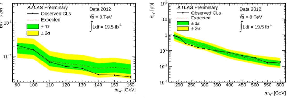
7 Results
The background and signal model is used in a binned, extended maximum likelihood fit [61] to the
data. The parameter of interest in the fit is either the branching fraction B(t
→H
+b) (light H
+) or the
production cross section
σ(pp
→t(b)H
+) (heavy H
+). Systematic uncertainties are included as nuisance
pτT=(40,70) GeV pτT=(70,500) GeV ETmiss=(65,80) GeV 0.94±0.16±0.18 0.89±0.14±0.26 ETmiss=(80,100) GeV 1±0.1±0.4 1.1±0.15±0.24 ETmiss=(100,500) GeV 0.93±0.09±0.18 0.94±0.10±0.31
Table 7: Scale factors measured for the
τhad−vis + ETmisstrigger efficiency. The first uncertainties are statistical, the second ones are systematic.
parameters in the likelihood function. A profile likelihood ratio [61] is used with the m
Tdistribution as the discriminating variable. The ˜ q
µtest statistic is used, based on a one-sided profile likelihood ratio.
Before applying the likelihood fit to the signal region data, the fitting method is validated by applying it to data and a model of the signal and background passing the event selection of the previously defined zero b-tags validation region. This region is orthogonal to the signal region. Its background composition is slightly different than the signal region, as the real
τhad−visbackground component is dominated by events from W boson
+jets events rather than tt. The fit model is able to describe the data well, and there is no evidence of significant signal in this validation region, as expected. The observed pulls of the nuisance parameters are also investigated in the validation region and, later, the signal region, where they are seen to be well-behaved.
[GeV]
mT
0 100 200 300 400 500 600
Events / 20 GeV
0.2 0.4 0.6 0.8 1 1.2 1.4 1.6 1.8 2
103
×
Selection H+ Light Data 2012
τ True
misID τ
→ Jet Uncertainty
= 130 GeV ( x 10)
H+
m
) = 0.9%
bH+
→ t B(
Ldt = 19.5 fb-1
∫
= 8 TeV s ATLAS Preliminary
[GeV]
mT
0 100 200 300 400 500 600
Events / 20 GeV
0.5 1 1.5 2 2.5 3
103
×
Selection H+ Heavy Data 2012
τ True
misID τ
→ Jet Uncertainty
= 250 GeV ( x 10)
H+
m
max
) = 50, MSSM mh
β tan(
Ldt = 19.5 fb-1
∫
= 8 TeV s ATLAS Preliminary
[GeV]
mT
0 100 200 300 400 500 600
Events / 20 GeV
1 10 102
103
104
105
Selection H+ Light Data 2012
τ True
misID
→τ Jet Uncertainty
= 130 GeV ( x 10)
H+
m
) = 0.9%
bH+
→ t B(
Ldt = 19.5 fb-1
∫
= 8 TeV s ATLAS Preliminary
[GeV]
mT
0 100 200 300 400 500 600
Events / 20 GeV
1 10 102
103
104
105
Selection H+ Heavy Data 2012
τ True
misID τ
→ Jet Uncertainty
= 250 GeV ( x 10)
H+
m
max h
) = 50, MSSM m β
tan(
Ldt = 19.5 fb-1
∫
= 8 TeV s ATLAS Preliminary
Figure 5: The data and background predictions after applying the nominal selection for the (left) light
charged Higgs boson search and for the (right) heavy charged Higgs boson search. They are shown both
in linear scale (top) and logarithmic scale (bottom). In the distributions for the light
H+signal selection,
a signal of
mH+ =130 GeV and
B(t→ H+b) =0.9% is included. For the heavy
H+signal selection, a
signal of
mH+ =250 GeV and tan
β =50 with the cross section and
B(H+ → τν) of the MSSMmmaxhscenario [59] is included. All signal contributions are scaled up by a factor of 10. The last bin of each
mTdistribution includes overflow. The uncertainty band shows the pre-fit systematic uncertainties, added in
quadrature.
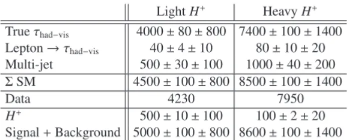
The fit model is then applied to the data in the signal region. The data, compared to the background predictions, are shown in Fig. 5 for the light and heavy charged Higgs boson nominal selection criteria.
The total expected and observed yields are shown in Table 8. For the light H
+selection, a signal of m
H+ =130 GeV and B(t
→H
+b)
=0.9% is included. For the heavy H
+selection, a signal of m
H+ =250 GeV and tan
β =50 with the cross section and B(H
+ → τν) of the MSSMm
maxhscenario [59] is included.
LightH+ HeavyH+
Trueτhad−vis 4000±80±800 7400±100±1400
Lepton→τhad−vis 40±4±10 80±10±20 Multi-jet 500±30±100 1000±40±200 ΣSM 4500±100±800 8500±100±1400
Data 4230 7950
H+ 500±10±100 100±2±20 Signal+Background 5000±100±800 8600±100±1400