Search for pair-produced top squarks decaying into charm quarks and the lightest neutralinos using 20.3 fb

ATLAS-CONF-2013-068 18July2013

ATLAS NOTE

ATLAS-CONF-2013-068

July 17, 2013

Search for pair-produced top squarks decaying into charm quarks and the lightest neutralinos using 20.3 fb

⁻¹

of pp collisions at √

s = 8 TeV with the ATLAS detector at the LHC

ATLAS Collaboration

Abstract

This note presents the search for direct top squark pair production in the decay channel to a charm quark and the lightest neutralino (˜

t→c+χ

˜

⁰₁

), using 20.3 fb

⁻¹

of proton-proton collision data at

√

s=

8 TeV recorded by the ATLAS experiment at the LHC in 2012. The analysis is carried out in different signal regions according to the final state jet multiplicity.

One of the regions uses charm-flavour identification to increase the signal purity. No ex- cess above the Standard Model background expectation is observed. Limits are set on the visible cross-section of new physics within the requirements of the search. The results are interpreted in the context of direct pair production of top squarks and presented in terms of exclusion limits in the (m

˜t

,

m_χ˜⁰

1

) plane. A top squark mass of 200 GeV is excluded at 95%

confidence level for

mt˜

–m

_χ˜⁰

1 <

85 GeV. Top squark masses up to 230 GeV are excluded for a neutralino mass of 200 GeV. This extends significantly previous Tevatron results.

c Copyright 2013 CERN for the benefit of the ATLAS Collaboration.

1 Introduction

Supersymmetry (SUSY) [1–9] is a theoretically favoured candidate for physics beyond the Standard Model (SM). It naturally solves the hierarchy problem and provides a possible candidate for dark mat- ter in the universe. SUSY doubles the SM spectrum of particles by introducing a new supersymmetric partner (sparticle) for each particle in the SM. In particular, a new scalar field is associated with each left- and right-handed quark state, and two squark mass eigenstates ˜ q

₁

and ˜ q

₂

result from the mixing of the scalar fields. In some SUSY scenarios, a significant mass difference between eigenstates in the top squark (stop) sector can occur, leading to a rather light stop ˜ t

1

mass state. In addition, naturalness argu- ments suggest that the third generation sfermions should be light with masses below 1 TeV. In a generic minimal supersymmetric extension of the SM (MSSM) that assumes R-parity conservation, sparticles are produced in pairs and the lightest supersymmetric particle (LSP) is stable and identified as the lightest neutralino ˜

χ⁰₁

.

For a mass difference

∆m =

m

t˜−

m

_χ˜⁰

1 >

m

_t

, and depending on the SUSY parameters and mass hierarchy, the dominant decay channels are ˜ t

→

t

+ χ

˜

⁰₁

or ˜ t

→

b

+χ

˜

^±₁

, where the latter involves the presence of charginos ( ˜

χ^±₁

) which subsequently decay into the lightest neutralino via a W

^(∗)

emission. If the chargino is heavier than the stop and m

_W +

m

_b < ∆m <

m

_t

, the dominant decay mode is expected to be the three-body Wb

χ

˜

⁰₁

decay. Several searches on 2011 data have been carried out in these decay channels in 0 to 2 lepton final states [10–12] and have been extended in 2012 [13–16]. In the scenario for which

∆m<

m

W +

m

b

, the dominant decay mode can be a stop decay to a charm quark and the LSP (˜ t

→

c

+χ

˜

⁰₁

), which proceeds via a loop decay (see Fig. 1). The corresponding final state is characterized by the presence of two jets from the hadronization of the charm quarks and missing transverse momentum (denoting its magnitude by E

^miss_T

) from the two undetected LSPs. However, given the relatively small mass difference (∆m), both the transverse momenta of the two charm jets and the E

_T^miss

are too low to extract this signal from the large multijet background.

In this study, the event selection makes use of the presence of initial-state radiation (ISR) jets to identify signal events. Two different approaches are used to target the different

∆m

regions. For small

∆m,

Figure 1: Feynman diagram for the pair production of top squarks with subsequent decay to charm quarks and two LSP’s.

the approach follows closely the “monojet” analysis of Ref. [17], where events with low jet multiplicity

and large missing transverse momentum are selected. For moderate

∆m

the charm jets receive a large

enough boost to be detected. In addition to the requirements on the presence of ISR jets, charm tagging

is used, for the first time at the LHC, to enhance the SUSY signal. Results on searches in this channel using Tevatron data have been previously reported by both the CDF and D0 experiments [18, 19].

2 Monte Carlo simulation

Monte Carlo (MC) simulation samples are used to aid in the description of the background and to model the stop signal. The MC samples are processed either with a full ATLAS detector simulation [20] based on the Geant4 program [21] or a fast simulation based on the parameterization of the response of the electromagnetic and hadronic showers in the ATLAS calorimeters [22]. The effect of multiple pp inter- actions in the same or nearby bunch crossing is also simulated.

The Sherpa [23] generator is used to simulate W+jets and Z/γ

^∗+jets processes, assuming massive

b/c-quarks, and the Alpgen [24] generator is employed to assess the corresponding modelling uncer- tainties. Production of top quark pairs is simulated with Powheg [25]. The Alpgen and MC@NLO [26]

generators are used to assess the t t ¯ modelling uncertainty. Single top samples are generated with MC@NLO for the s– and Wt–channel while AcerMC [27] is used for single top production in the t–channel. Fi- nally, t¯ t samples with additional vector bosons are generated with Madgraph [28]. A top quark mass of 172.5 GeV is used consistently. Diboson samples (WW , WZ and ZZ production) are generated using Sherpa. Additional samples are generated with Herwig [29] to assess uncertainties. In case of Powheg and Madgraph, parton showers are implemented using Pythia [30, 31], and Herwig plus Jimmy [32] is used for the Alpgen and MC@NLO generators. The multijet background is determined from the data. For cross checks, dijet samples are generated with Pythia.

The cross sections for Z/γ

^∗

, W and t¯ t production at

√

s

=

8 TeV are known at (approximate) next- to-next-to-leading order (NNLO) in perturbative QCD (pQCD): the values are 1.12

±

0.04 nb, 12.19

±

0.52 nb and 238

⁺²²₋₂₄

pb, for Z/γ

^∗

(

→ ℓℓ),

W

→

(ℓν) and t t, respectively. The ¯ Z/γ

^∗

and W cross sections have been calculated with DYNNLO [33, 34] using MSTW2008 90% NNLO parton density function (PDF) sets [35]. The cross section for top pair production is calculated with Hathor 1.2 [36] using the MSTW2008 90% NNLO PDF sets incorporating PDF+α

S

uncertainties, according to the MSTW prescription [37]. This is added in quadrature to the scale uncertainty and cross checked with the NLO+NNLL calculation [38] as implemented in Top++ 1.0 [39]. The single top cross sections are 5.6

±

0.2 pb [40], 87.8

^+3.4_−1.9

pb [41] and 22.4

±

1.5 pb [42] for the s-channel, t-channel and Wt-channel, respectively. Finally, the cross sections for top pair production in association with a W or Z boson are known at NLO precision and are 0.231

±

0.046 pb and 0.206

±

0.021 pb for t¯ tW and t¯ tZ, respectively [43].

For WW , WZ, and ZZ production, NLO cross sections of 57.3

^+2.3_−1.6

pb, 21.5

^+1,1_−0.9

pb, and 7.92

^+0.37_−0.24

pb [44], respectively, are used.

Stop pair production with ˜ t

→

c

+χ

˜

⁰₁

is modelled with Madgraph with one additional jet from the matrix element. The showering is done with Pythia. Stop masses are produced between 100 GeV and 300 GeV in steps of 25 GeV and between 300 GeV and 400 GeV in steps of 50 GeV. ˜

χ⁰₁

masses are produced between 70 GeV and 390 GeV with a minimum mass difference of 5 GeV. The

∆m

step size increases with

∆m

from 5 GeV to 30 GeV. Signal cross sections are calculated to NLO in pQCD, adding the resummation of soft gluon emission at next-to-leading-logarithmic (NLO+NLL) accuracy [45–47].

The nominal cross section and the uncertainty are taken from an envelope of cross section predictions

using different PDF sets and factorization and renormalization scales, as described in Ref. [48].

3 Reconstruction of physics objects

Jets are reconstructed from energy deposits in calorimeters using the anti-k

_t

jet algorithm [49] with the distance parameter (in

η−φ

space)

¹

set to R

= p

∆η²+ ∆φ²=

0.4. The measured jet transverse momen- tum ( p

T

) is corrected for detector effects, including the non-compensating character of the calorimeter, by reweighting differently energy deposits arising from electromagnetic and hadronic showers. In addition, jets are corrected for contributions from multiple proton-proton interactions per beam bunch crossing (pileup), as described in Ref. [50]. E

_T^miss

is reconstructed using all energy deposits in the calorimeter up to a pseudorapidity

|η|

of 4.9. These clusters are calibrated taking into account the difference in response of jets compared to electrons or photons, as well as dead material and out-of-cluster energy losses [51].

Electron candidates are required to have p

T >

20 GeV and

|η| <

2.47, and to pass the medium electron shower shape and track selection criteria described in Ref. [52] and reoptimized for 2012 data. Muon candidates are required to have p

_T >

10 GeV and

|η|<

2.5 and to pass the combined reconstruction cri- teria described in Ref. [53–55], which include the association of a stand-alone muon spectrometer track to an inner detector track. Overlaps between identified leptons and jets in the final state are resolved.

Jets are discarded if their distance

∆R

to an identified electron is less than 0.2. For the remaining jets in the events the electrons between 0.2 and 0.4 from a jet are removed. Similarly, muons are required to have

∆R>

0.4 with respect to any selected jet in the event. In addition, as discussed below, the leptons used to veto events in the signal regions or to define control regions in data are required to be isolated. In the case of electrons, the total transverse momentum not associated with the electron in a cone of radius 0.2 around the electron candidate must be less than 10% of the electron’s transverse momentum. For the muons, the sum of the transverse momenta of the tracks not associated with the muon is required to be less than 1.8 GeV.

3.1 Charm tagging

Jets are identified as originating from the hadronization of a charm quark (c-tagging) via a dedicated al- gorithm using multivariate techniques to combine information from the impact parameters of displaced tracks and topological properties of secondary and tertiary decay vertices reconstructed within the jet.

The algorithm provides three weights, one targeted for light-flavor quarks and gluon jets (P

u

), one for charm jets (P

_c

) and one for b-jets (P

_b

). From these weights, anti-b and anti-u discriminators are calcu- lated (see Fig. 2):

anti-b

≡

log P

_c

P

b

!

and anti-u

≡

log P

_c

P

u

! ,

and applied to the selected jets in the final state. Two operating points specific to c-tagging are used.

The medium operating point (log

_P

c

Pb

> −

1, log

_P

c

Pu

> −

0.82) has a c-tagging efficiency of

≈

20%, and a rejection factor of

≈

5 for b-jets,

≈

140 for light-flavor jets, and

≈

10 for tau-jets. The loose operating point (log

_P

c

Pb

>−

1) has a c-tagging efficiency of

≈

95%, with a factor of 2 rejection of b-jets but without any significant rejection of light-flavor or tau jets. The efficiencies and rejections are quoted for simulated t t ¯ events for jets with 30 GeV

<

p

T <

200 GeV and

|η| <

2.5. The c-tagging efficiency is calibrated using data and the method described in Ref. [56]. The same method applied to the 8 TeV data leads to reduced uncertainties. The standard calibration techniques are used for the b-jet [57] and light-jet [58] rejections.

1ATLAS uses a right-handed coordinate system with its origin at the nominal interaction point (IP) in the centre of the detector and thez-axis along the beam pipe. Thex-axis points from the IP to the centre of the LHC ring, and they-axis points upward. Polar coordinates (r, φ) are used in the transverse (x,y)-plane,φbeing the azimuthal angle around the beam pipe. The rapidity is defined asy=0.5×ln[(E+pz)/(E−pz)], whereEdenotes the energy andpzis the component of the momentum along the beam direction. The pseudorapidity is defined in terms of the polar angleθasη=−ln tan(θ/2).

Events / 0.5

10-1

1 10 102

103

104

105

106

Data 2012 Standard Model

) +jets l ν W ( →

(+X) + single top t

t

) +jets ν ν

→ Z (

ll ) +jets

→ Z ( dibosons ATLASPreliminary

∫Ldt = 20.3 fb^{-1, s = 8 TeV}

u)

c/P leading jet log(P

-8 -6 -4 -2 0 2 4 6

Data / SM

0 1 2

Events / 0.5

10-1

1 10 102

103

104

105

106

Data 2012 Standard Model

) +jets l ν W ( →

(+X) + single top t

t

) +jets ν ν

→ Z (

ll ) +jets

→ Z ( dibosons ATLASPreliminary

∫Ldt = 20.3 fb^{-1, s = 8 TeV}

u)

c/P fourth leading jet log(P

-8 -6 -4 -2 0 2 4 6

Data / SM

0 1 2

Events / 0.5

10-1

1 10 102

103

104

105

106

Data 2012 Standard Model

) +jets ν

→ l W (

(+X) + single top t

t

) +jets ν ν Z ( →

ll ) +jets Z ( → dibosons ATLASPreliminary

∫Ldt = 20.3 fb^{-1, s = 8 TeV}

b)

c/P second leading jet log(P

-10 -8 -6 -4 -2 0 2 4

Data / SM

0 1 2

Events / 0.5

10-1

1 10 102

103

104

105

106

Data 2012 Standard Model

) +jets ν

→ l W (

(+X) + single top t

t

) +jets ν ν Z ( →

ll ) +jets Z ( → dibosons ATLASPreliminary

∫Ldt = 20.3 fb^{-1, s = 8 TeV}

b)

c/P third leading jet log(P

-10 -8 -6 -4 -2 0 2 4

Data / SM

0 1 2

Figure 2: (Top) Distribution of the discriminator against light-jets, log(P

_c/P_u

), for the leading (left)

and fourth leading jet (right). (Bottom) Distribution of the discriminator against b-jets, log(P

_c/Pb

), for

the second (left) and third leading jet (right). The discriminators shown for the different jets follow

the tagging criteria discussed in Section 4. The data are compared to MC simulations for the different

SM processes and include the signal selection C1 defined in Section 4 without applying the tagging

requirements. The error bands in the ratios include the statistical and experimental uncertainties in the

predictions.

4 Event selection

The data sample used in this note was collected with the ATLAS detector and corresponds to a total integrated luminosity of 20.3 fb

⁻¹

. The uncertainty on the integrated luminosity is

±

2.8%. It is estimated, following the same methodology as that detailed in Ref. [59], from a preliminary calibration of the luminosity scale derived from beam-separation scans performed in November 2012. The data were selected online using a trigger logic that selects events with E

_T^miss

above 80 GeV, as computed at the final stage of the three-level trigger system of ATLAS [60]. With respect to the analysis requirements, the trigger selection is fully efficient, as determined using a data sample with muons in the final state. The following preselection criteria are applied.

•

Events are required to have a reconstructed primary vertex [61] consistent with the beamspot en- velope and having at least five tracks; when more than one such vertex is found, the vertex with the largest summed

|

p

_T|²

of the associated tracks is chosen. This rejects beam-related backgrounds and cosmic rays.

•

Events are required to have E

^miss_T >

150 GeV and at least one jet with p

_T >

120 GeV and

|η|<

2.8 in the final state.

•

Events are rejected if they contain any jet with p

_T>

20 GeV and

|η|<

4.5 that presents anomalous charged fraction, electromagnetic fraction in the calorimeter, or sampling fraction inconsistent with the requirement that they originate from a proton-proton collision. In the case of the leading jet in the event, the requirements are tightened to reject potentially remaining contributions from beam- related backgrounds and cosmic rays. Additional requirements are applied to suppress coherent noise and electronic noise bursts in the calorimeter producing anomalous energy deposits [62].

•

Events with isolated electrons (muons) with p

T >

20 GeV (p

T >

10 GeV) are vetoed.

4.1 Monojet-like selection

The monojet-like analysis targets the region in which stop and lightest neutralino are nearly degenerate in mass so that c-jets are too soft to be tagged. Stop pair production events are then characterized by a small number of jets and can be identified via the presence of an energetic jet from initial state radiation. A maximum of three jets with p

T >

30 GeV and

|η|<

2.8 in the event is allowed. An additional requirement on the azimuthal separation of

∆φ(jet,p^miss_T

)

>

0.4 between the missing transverse momentum direction and that of each of the selected jets is set. This requirement reduces the multijet background contribution where the large E

_T^miss

originates from mainly jet mismeasurement. A signal region (denoted M1) is defined with leading jet p

_T >

280 GeV and E

^miss_T >

220 GeV, as the result of an optimization performed as a function of the ˜ t and ˜

χ⁰₁

masses.

4.2 Charm-tagged selection

While the monojet-like selection has a relatively small signal to background ratio, the charm-tagged selection is designed to enhance the signal purity in the moderate

∆m

region. The kinematics of the charm jets from the stop decays depend mainly on

∆m. As∆m

decreases, the p

T

’s of the charm jets become softer and it is more likely that more than one jet from initial state radiation has a higher transverse momentum than the charm jets. An optimization of the charm-tagged selection criteria is performed across the ˜ t and ˜

χ⁰₁

mass plane to maximize the sensitivity to a SUSY signal.

A signal region (denoted C1) is defined by requiring E

^miss_T >

410 GeV and a leading jet with p

T >

270 GeV and

|η|<

2.8. Three additional jets are required to have p

_T >

30 GeV and

|η| <

2.5. As in the

monojet-like case, the azimuthal separation

∆φ(jet,p^miss_T

)

>

0.4 between the E

^miss_T

direction and that of each of the selected jets is required. Different tagging approaches are applied to the different jets. The leading jet tends to be an ISR jet, both for signal and background. Therefore, no tagging requirement is applied. The second and third leading-jets are required to have a loose charm-tag and the fourth leading jet is required to pass the medium charm-tagging requirement. The loose tags represent a b-jet veto which mainly serves to reject t¯ t background, and the medium tag represents both a b-jet and a light-jet veto. It is applied to the fourth leading jet which is likely to be a charm-jet originating from a stop decay. While the ISR jet is selected in the region

|η| <

2.8, the tagged jet requirement is tightened to

|η| <

2.5 to be within the acceptance of the inner tracking detector.

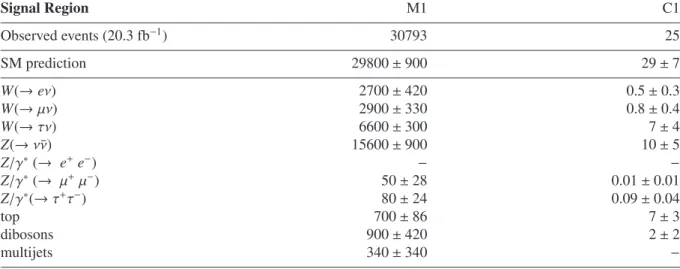
Table 1 summarizes the different event selection criteria applied in the signal regions.

Selection criteria Preselection

Primary vertex

E^miss_T >120 GeV Jet quality requirements

At least one jet withpT>120 GeV and|η|<2.8

Lepton vetoes: no isolated electrons (muons) withpT>20 GeV (pT >10 GeV)

Monojet-like selection M1 Charm-tagged selection C1

At most three jets withpT>30 GeV and|η|<2.8 At least three jets with pT >30 GeVand|η|< 2.5 (in addition to the leading jet)

b-veto for second and third jet medium c-tag for fourth jet

∆φ(jet,p^miss_T )>0.4 ∆φ(jet,p^miss_T )>0.4

minimum leading jetp_T(GeV) 280 270

minimumE^miss_T (GeV) 220 410

Table 1: Event selection criteria applied for the monojet-like and charm-tagged analyses.

5 Background estimation

The expected SM background is dominated by Z (

→ν¯ν)+jets,

t¯ t and W(

→ℓν)+jets (ℓ=

e, µ, τ) produc- tion, and include contributions from Z/γ

^∗

(

→ℓ⁺ℓ⁻

)+jets, multijet and diboson (WW, WZ, ZZ) processes.

The W/Z plus jets backgrounds are estimated using MC event samples normalized using data in control regions. The top background contribution to the monojet-like analysis is very small and determined us- ing MC simulated samples. In the case of the charm-tagged analysis the top background is sizable, as enhanced by the c-tagged requirements, and is estimated using MC simulated samples normalized in a top-enriched control region. The remaining SM backgrounds from dibosons are determined using Monte Carlo simulated samples, while the multijet background contribution is extracted from data. The normal- ization factors for the different background contributions are extracted simultaneously using a global fit to all control regions and including systematic uncertainties, to properly take into account correlations.

Finally, the potential contributions from beam-related background and cosmic rays are estimated using data and found to be negligible.

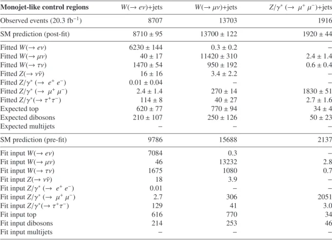
5.1 Electroweak background

In the monojet-like analysis, control samples in data, orthogonal to the signal region, with identified

toes, and E

^miss_T

, are used to determine the W

/Z+jets electroweak background contributions from data.

This reduces significantly the relatively large theoretical and experimental systematic uncertainties as- sociated to purely MC-based predictions. A W(

→µν)+jets control sample is defined using events with

a muon with p

T >

10 GeV and transverse mass

²

in the range 30 GeV

<

m

T <

100 GeV. Similarly, a Z/γ

^∗

(

→ µ⁺µ⁻

)+jets control sample is selected requiring the presence of two muons with invariant mass in the range 66 GeV

<

m

_µµ <

116 GeV. Finally, a W(

→

eν)+jets dominated control sample is defined using events with an electron candidate with p

T >

20 GeV. For the latter, the E

_T^miss

calculation includes the contribution of the energy cluster from the identified electron in the calorimeter, that is treated as a jet, since W(

→

eν)+jets processes contribute to the background in the signal region when the electron is not identified. In the W(

→µν)+jets and

Z/γ

^∗

(

→ µ⁺µ⁻

)+jets control regions the E

^miss_T

does not include muon contributions as they are considered invisible.

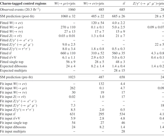
The definition of the control regions in the charm-tagged analysis follows closely that of the monojet- like approach. A tighter cut 81 GeV

<

m

µµ<

101 GeV is used to define the Z/γ

^∗

(

→ µ⁺µ⁻

)+jets control sample, as required to further reject t t ¯ contamination. In the charm-tagged analysis, the c-tagging is one of the major uncertainties and the same tagging criteria as used in the signal selection are applied to the W(

→ µν)+jets,

W(

→

eν)+jets and Z/γ

^∗

(

→ µ⁺ µ⁻

)+jets control regions. Since this increases significantly the statistical uncertainty in these control regions, the kinematic selections on the leading jet p

_T

and E

_T^miss

are both reduced to 150 GeV for which the trigger selection still remains fully efficient.

This implies the need for a MC-based extrapolation of the normalization factors, as determined using data at relatively low leading jet p

T

and E

^miss_T

, to the signal region. The W/Z+jets MC samples in the charm-tagged analysis are reweighted to ensure that they properly describe the measured boson p

_T

distribution in the data, following the same procedure as described in Ref. [63], and leading to a very good description of the shape of the measured jet p

T

and E

_T^miss

distributions.

Monte Carlo-based transfer factors, determined by the Sherpa simulation, are defined for each of the signal selections to estimate the different electroweak background levels in the signal regions. As an example, in the case of the dominant Z(

→ ν¯ν)+jets background process, its contribution to a given

signal region N(Z(

→ ν¯ν)+

jets)

_signal

would be determined using the W(

→ µν)+jets control sample in

data according to

N(Z(

→ν¯ν)+

jets)

_signal =

(N

_W^data_{→µν,control}−

N

_W^non_→⁻_µν,control^W

)

×

N

^MC

(Z(

→ν¯ν)+

jets)

_signal

N

_W^MC_{→µν,control} ,

(1) where N

^MC

(Z(

→ ν¯ν)+

jets)

signal

denotes the background predicted by the MC simulation in the signal region, and N

_W^data_{→µν,control}

, N

_W^MC_{→µν,control}

, and N

_W^non_→⁻_µν,control^W

denote, in the control region, the number of W(

→µν)+jets candidates in data and MC simulation, and the non-W(→ µν) background contribution,

respectively. The latter refers mainly to top-quark and diboson processes, but also includes contributions from the rest of W

/Z+jets processes. Therefore, the transfer factors for each process are defined as the

ratio of simulated events for the process in the signal region over the total number of simulated events in the control region.

In the monojet-like analysis, the W(

→µν)+jets control sample is employed to define transfer factors

for W(

→µν)+jets and

Z (

→ ν¯ν)+jets processes, and the

W(

→

eν)+jets control sample is used to con- strain W(

→

eν)+jets, W(

→τν)+jets,

Z/γ

^∗

(

→τ⁺τ⁻

)+jets, and Z/γ

^∗

(

→

e

⁺

e

⁻

)+jets contributions. The Z/γ

^∗

(

→ µ⁺µ⁻

)+jets control sample is used to constrain the Z/γ

^∗

(

→ µ⁺µ⁻

)+jets background contri- bution and as an alternate estimate of the Z(

→ν¯ν)+jets and the rest of

Z/γ

^∗

(

→ℓ⁺ℓ⁻

)+jets background contributions (see Section 6). The charm-tagged analysis follows a similar approach to determine the nor- malization factors for each of the W/Z+jets background contributions. However, in this case the nominal

2The transverse massmTis defined by the lepton (ℓ) and neutrino (ν)pTand direction asmT= q

2p^ℓ_Tp^ν_T(1−cos(φ^ℓ−φ^ν)), where the (x, y) components of the neutrino momentum are taken to be the same as the correspondingE_T^misscomponents.

Z(

→ ν¯ν)+jets normalization is extracted from the

Z/γ

^∗

(

→ µ⁺ µ⁻

)+jets control sample, motivated by the fact that both processes involve identical heavy flavor production mechanisms.

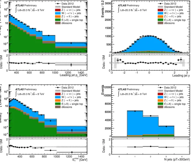
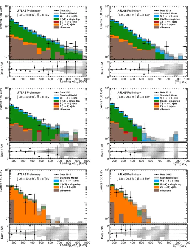
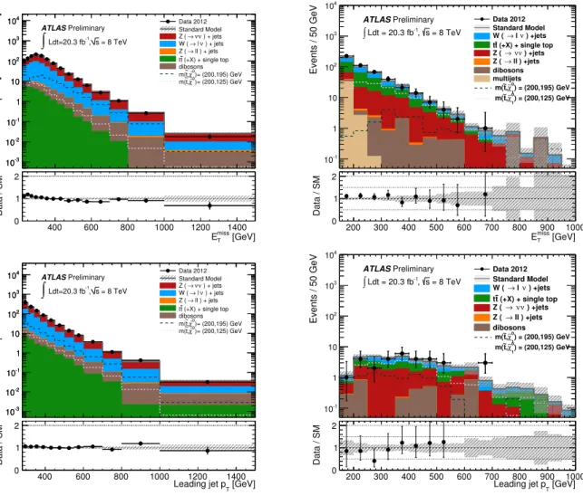
Figures 3-5 show, for the different control samples, a number of selected distributions in data and MC simulations for the M1 selection. Similarly, the distribution of the leading jet p

T

and E

^miss_T

in the three control regions for the C1 selection are shown in Fig. 6. The W

/Z+jets predictions are obtained

using Sherpa and include the data-driven normalization factors.

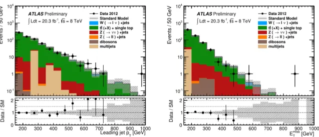
5.2 Top quark background

As already mentioned, the background contribution of top quark production processes to the monojet- like selection is small and is enterely determined from MC. In the case of the charmed-tagged analysis, the MC predictions are normalized to the data in a separate control region. For this t¯ t control region, b-tagging is used to yield a high-purity control region with negligible signal contamination. In addition to lowering the leading jet p

T

and E

_T^miss

requirements both to 150 GeV, c-tagging is replaced by b-tagging by inverting the loose c-tagging criterion: the inverted b-veto is thereby converted into a b-identification requirement. For this control region, at least two b-tagged jets among the three leading jets need to be identified. The distributions of the leading jet p

T

and E

^miss_T

for this t t ¯ control region are shown in Fig. 7.

5.3 Multijets background

The multijet background events can enter the signal regions if one of the jets is mis-measured, producing fake E

^miss_T

, and from events containing true E

_T^miss

(neutrinos from heavy flavour decays). The background is determined mainly from data, with minimal dependence on the MC simulation. This technique, which is referred to as the jet smearing method, has been used in other SUSY searches [64]. It relies on the assumption that the E

^miss_T

of multijet events is dominated by jet fluctuations (true or fake) and that those fluctuations can be measured in the data. The method proceeds as follows:

1. A sample of low-E

^miss_T

seed events is selected from data.

2. A response function, R, which quantifies the fluctuation in measured jet p

_T

, is measured. This re- sponse function includes effects of jet mis-measurements and contribution from neutrinos in heavy flavour decays. An initial estimate of the response function is obtained from the MC simulation.

3. The response function is modified by smearing the seed events, until good agreement is observed between smeared data and data in control regions sensitive to this jet response.

4. Seed events are then smeared with the adjusted response function from (3).

Seed events are selected with single jet triggers and low E

_T^miss

significance, E

_T^miss/√P

E

T

, where

P

E

T

denotes the scalar sum of the transverse energy in the detector. Here E

^miss_T

significance is preferred over E

^miss_T

itself to avoid biasing the jet p

_T

distribution. Two response functions are used, one for jets with b-veto and another for b-tagged jets. At least 250 smeared events are produced from each seed event.

These events are normalised to data in a multijet dominated control region, defined by small

∆φ(jet, p^miss_T

). The contribution from other backgrounds is subtracted using MC simulations. This sample is

then used to estimate the multijets background in the different selections. For the monojet-like analysis,

it constitutes less than 1% of the total background and it is negligible in the charm-tagged case.

400 600 800 1000 1200 1400 [ Events / GeV ] TdN/dp

10-3

10-2

10-1

1 10 102

103

104 _{Data 2012}

Standard Model ) + jets ν ν

→ Z (

) + jets ν

→ l W (

ll ) + jets

→ Z (

(+X) + single top t

t dibosons = 8 TeV

s

-1, Ldt=20.3 fb

∫

ATLASPreliminary

400 600 800 1000 1200 1400

[ Events / GeV ] TdN/dp

10-3

10-2

10-1

1 10 102

103

104

[GeV]

Leading jet pT

400 600 800 1000 1200 1400

Data / SM

0 1

2 -3 -2 -1 0 1 2 3

Events / 0.2

0 500 1000 1500 2000 2500

3000 Data 2012

Standard Model ) + jets ν ν

→ Z (

) + jets ν

→ l W (

ll ) + jets

→ Z (

(+X) + single top t

t dibosons = 8 TeV

s

-1, Ldt=20.3 fb

∫

ATLASPreliminary

-3 -2 -1 0 1 2 3

Events / 0.2

0 500 1000 1500 2000 2500 3000

Leading jet y

-3 -2 -1 0 1 2 3

Data / SM

0 1 2

400 600 800 1000 1200 1400

[ Events / GeV ]TmissdN/dE

10-3

10-2

10-1

1 10 102

103

Data 2012 Standard Model

) + jets ν ν

→ Z (

) + jets ν

→ l W (

ll ) + jets

→ Z (

(+X) + single top t

t dibosons = 8 TeV

s

-1, Ldt=20.3 fb

∫

ATLASPreliminary

400 600 800 1000 1200 1400

[ Events / GeV ]TmissdN/dE

10-3

10-2

10-1

1 10 102

103

[GeV]

T

Emiss

400 600 800 1000 1200 1400

Data / SM

0 1

2 0 1 2 3 4

Events

0 2000 4000 6000 8000 10000

12000 Data 2012

Standard Model ) + jets ν ν

→ Z (

) + jets ν

→ l W (

ll ) + jets

→ Z (

(+X) + single top t

t dibosons = 8 TeV

s

-1, Ldt=20.3 fb

∫

ATLASPreliminary

0 1 2 3 4

Events

0 2000 4000 6000 8000 10000 12000

N jets (pT>30GeV)

0 1 2 3 4

Data / SM

0 1 2

Figure 3: The leading jet p

_T

and

y,

E

^miss_T

, and jet multiplicity distributions in the W(

→µν)+jet control

region, for the M1 selection, compared to the background predictions. The latter include the global

normalization factors extracted from the fit (see Section 6). The error bands in the ratios include the

statistical and experimental uncertainties on the background predictions.

400 600 800 1000 1200 1400 [ Events / GeV ] TdN/dp

10-3

10-2

10-1

1 10 102

103 Data 2012

Standard Model ) + jets ν

→ l W (

ll ) + jets Z ( →

(+X) + single top t

t dibosons = 8 TeV

s

-1, Ldt=20.3 fb

∫

ATLASPreliminary

400 600 800 1000 1200 1400

[ Events / GeV ] TdN/dp

10-3

10-2

10-1

1 10 102

103

[GeV]

Leading jet pT

400 600 800 1000 1200 1400

Data / SM

0 1

2 -3 -2 -1 0 1 2 3

Events / 0.2

0 50 100 150 200 250 300 350 400

450 Data 2012

Standard Model ) + jets ν

→ l W (

ll ) + jets Z ( →

(+X) + single top t

t dibosons = 8 TeV

s

-1, Ldt=20.3 fb

∫

ATLASPreliminary

-3 -2 -1 0 1 2 3

Events / 0.2

0 50 100 150 200 250 300 350 400 450

Leading jet y

-3 -2 -1 0 1 2 3

Data / SM

0 1 2

400 600 800 1000 1200 1400

[ Events / GeV ]TmissdN/dE

10-3

10-2

10-1

1 10 102

103

Data 2012 Standard Model

) + jets l ν W ( →

ll ) + jets

→ Z (

(+X) + single top t

t dibosons = 8 TeV

s

-1, Ldt=20.3 fb

∫

ATLASPreliminary

400 600 800 1000 1200 1400

[ Events / GeV ]TmissdN/dE

10-3

10-2

10-1

1 10 102

103

[GeV]

T

Emiss

400 600 800 1000 1200 1400

Data / SM

0 1

2 0 1 2 3 4

Events

0 200 400 600 800 1000 1200 1400 1600

1800 Data 2012

Standard Model ) + jets l ν W ( →

ll ) + jets

→ Z (

(+X) + single top t

t dibosons = 8 TeV

s

-1, Ldt=20.3 fb

∫

ATLASPreliminary

0 1 2 3 4

Events

0 200 400 600 800 1000 1200 1400 1600 1800

N jets (pT>30GeV)

0 1 2 3 4

Data / SM

0 1 2

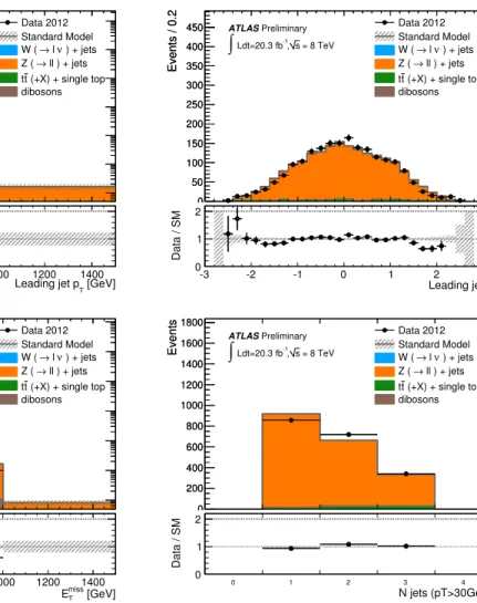
Figure 4: The measured leading jet p

_T

and

y,

E

^miss_T

, and jet multiplicity distributions in the Z/γ

^∗

(

→ µ⁺ µ⁻

)+jet control region, for the M1 selection, compared to the background predictions.

The latter include the global normalization factors extracted from the fit (see Section 6). The error bands

in the ratios include the statistical and experimental uncertainties on the background predictions.

400 600 800 1000 1200 1400 [ Events / GeV ] TdN/dp

10-3

10-2

10-1

1 10 102

103

Data 2012 Standard Model

) + jets ν ν

→ Z (

) + jets ν

→ l W (

ll ) + jets

→ Z (

(+X) + single top t

t dibosons = 8 TeV

s

-1, Ldt=20.3 fb

∫

ATLASPreliminary

400 600 800 1000 1200 1400

[ Events / GeV ] TdN/dp

10-3

10-2

10-1

1 10 102

103

[GeV]

Leading jet pT

400 600 800 1000 1200 1400

Data / SM

0 1

2 -3 -2 -1 0 1 2 3

Events / 0.2

0 200 400 600 800 1000 1200 1400 1600 1800

2000 Data 2012

Standard Model ) + jets ν ν

→ Z (

) + jets ν

→ l W (

ll ) + jets

→ Z (

(+X) + single top t

t dibosons = 8 TeV

s

-1, Ldt=20.3 fb

∫

ATLASPreliminary

-3 -2 -1 0 1 2 3

Events / 0.2

0 200 400 600 800 1000 1200 1400 1600 1800 2000

Leading jet y

-3 -2 -1 0 1 2 3

Data / SM

0 1 2

400 600 800 1000 1200 1400

[ Events / GeV ]TmissdN/dE

10-3

10-2

10-1

1 10 102

103

Data 2012 Standard Model

) + jets ν ν

→ Z (

) + jets ν

→ l W (

ll ) + jets

→ Z (

(+X) + single top t

t dibosons = 8 TeV

s

-1, Ldt=20.3 fb

∫

ATLASPreliminary

400 600 800 1000 1200 1400

[ Events / GeV ]TmissdN/dE

10-3

10-2

10-1

1 10 102

103

[GeV]

T

Emiss

400 600 800 1000 1200 1400

Data / SM

0 1

2 0 1 2 3 4

Events

0 1000 2000 3000 4000 5000 6000 7000

Data 2012 Standard Model

) + jets ν ν

→ Z (

) + jets ν

→ l W (

ll ) + jets

→ Z (

(+X) + single top t

t dibosons = 8 TeV

s

-1, Ldt=20.3 fb

∫

ATLASPreliminary

0 1 2 3 4

Events

0 1000 2000 3000 4000 5000 6000 7000

N jets (pT>30GeV)

0 1 2 3 4

Data / SM

0 1 2

Figure 5: The measured leading jet p

_T

and

y,

E

_T^miss

, and jet multiplicity distributions in the W(

→

eν)+jet

control region, for the M1 selection, compared to the background predictions. The latter include the

global normalization factors extracted from the fit (see Section 6). The error bands in the ratios include

the statistical and experimental uncertainties on the background predictions.

Events / 50 GeV

10-1

1 10 102

103

104

Data 2012 Standard Model

) +jets ν

→ l W (

(+X) + single top t

t

) +jets ν ν

→ Z (

ll ) +jets

→ Z ( dibosons ATLASPreliminary

∫Ldt = 20.3 fb^{-1, s = 8 TeV}

[GeV]

Leading jet pT

200 300 400 500 600 700 800 900 1000

Data / SM

0 1 2

Events / 50 GeV

10-1

1 10 102

103

104

Data 2012 Standard Model

) +jets ν

→ l W (

(+X) + single top t

t

) +jets ν ν

→ Z (

ll ) +jets

→ Z ( dibosons ATLASPreliminary

∫Ldt = 20.3 fb^{-1, s = 8 TeV}

[GeV]

miss

ET

200 300 400 500 600 700 800 900 1000

Data / SM

0 1 2

Events / 50 GeV

10-1

1 10 102

103

104

Data 2012 Standard Model

) +jets ν

→ l W (

(+X) + single top t

t

) +jets ν ν

→ Z (

ll ) +jets

→ Z ( dibosons ATLASPreliminary

∫Ldt = 20.3 fb^{-1, s = 8 TeV}

[GeV]

Leading jet pT

200 300 400 500 600 700 800 900 1000

Data / SM

0 1 2

Events / 50 GeV

10-1

1 10 102

103

104

Data 2012 Standard Model

) +jets ν

→ l W (

(+X) + single top t

t

) +jets ν ν

→ Z (

ll ) +jets

→ Z ( dibosons ATLASPreliminary

∫Ldt = 20.3 fb^{-1, s = 8 TeV}

[GeV]

miss

ET

200 300 400 500 600 700 800 900 1000

Data / SM

0 1 2

Events / 50 GeV

10-1

1 10 102

Data 2012 Standard Model

) +jets ν

→ l W (

(+X) + single top t

t

ll ) +jets Z ( → dibosons ATLASPreliminary

∫Ldt = 20.3 fb^{-1, s = 8 TeV}

[GeV]

Leading jet pT

200 300 400 500 600 700 800 900 1000

Data / SM

0 1 2

Events / 50 GeV

10-1

1 10 102

Data 2012 Standard Model

) +jets ν

→ l W (

(+X) + single top t

t

ll ) +jets Z ( → dibosons ATLASPreliminary

∫Ldt = 20.3 fb^{-1, s = 8 TeV}

[GeV]

miss

ET

200 300 400 500 600 700 800 900 1000

Data / SM

0 1 2

Figure 6: The leading jet p

_T

and E

^miss_T

distributions for the c-tag W(

→ µν)+jets (top)

W(

→

eν)+jets (middle) and Z/γ

^∗

(

→ µ⁺ µ⁻

)+jets (bottom) control regions, compared to the background predictions.

The predictions include the global normalization factors extracted from the fit (see Section 6). The error

bands in the ratios include the statistical and experimental uncertainties on the background predictions.