A TLAS-CONF-2015-075 15 December 2015
ATLAS NOTE
ATLAS-CONF-2015-075
14th December 2015
Search for W W /W Z resonance production in the `ν q q final state at √
s = 13 TeV with the ATLAS detector at the LHC
The ATLAS Collaboration
Abstract
A search is presented for new resonances decaying to W W or W Z final states, where one W boson decays leptonically (to an electron or a muon, plus a neutrino) and the other W/Z boson decays hadronically. The data analysed comprises 3.2 fb − 1 of pp collision data at
√ s = 13 TeV, recorded with the ATLAS detector at the CERN Large Hadron Collider. No evidence for resonant diboson production is observed, and resonance masses below 1060 GeV and 1250 GeV are excluded at the 95 % confidence level for a spin-2 Randall-Sundrum bulk graviton and a possible new heavy vector boson coupling to the Higgs and the SM gauge bosons, respectively. The results are also interpreted in the context of an additional Higgs-like boson at high mass.
© 2015 CERN for the benefit of the ATLAS Collaboration.
Reproduction of this article or parts of it is allowed as specified in the CC-BY-4.0 license.
1 Introduction
Several scenarios of new physics beyond the Standard Model (SM), such as warped extra dimensions [1–
3], grand unified theories [4], and technicolour [5–7], predict new particles that predominantly decay to a pair of on-shell SM gauge bosons ( W/Z ). We present a search for such particles in the form of W W /W Z resonances where one W boson decays leptonically ( W → `ν with ` = e, µ ) and the other W /Z boson decays hadronically ( W/Z → q q ¯ 0 /q q ¯ with q, q 0 = u, d, c, s or b ). The analysis is based on 3 . 2 ± 0 . 2 fb − 1 of pp collision data at a centre-of-mass energy
√ s = 13 TeV, collected by the ATLAS experiment at the Large Hadron Collider (LHC). The search is optimized for a high mass resonance, where the two jets from a highly-boosted W or Z boson have a small opening angle and become difficult to distinguish using standard jet clustering algorithms. To mitigate the associated loss in efficiency, jets clustered with large radius parameters (large- R jets) are used and variables based on the substructure of these jets are employed.
Several signal models are used to optimize the analysis strategy and interpret the results. A heavy vector triplet (HVT) model, based on a simplified phenomenological Lagrangian [8], is used to model both W W and W Z resonances. Here, the new heavy vector boson, V 0 = W 0 , Z 0 , couples to the Higgs and the SM gauge bosons via a combination of parameters g V c H and to the fermions via the combination g 2 /g V c F . The redundancy of parameters is explicit, with g V representing the typical strength of the vector boson interaction, while the parameters c H and c F describe deviations from the nominal Higgs and fermion couplings, respectively, and are expected to be on the order of unity in most models. In this simplified model, all fermions are assumed to have the same coupling strength c F [8]. Other combinations of parameters, g V c V V V , g V 2 c V V H H and c V V W , control multiboson production and have a negligible impact on the overall cross sections for the processes of interest here.
A Kaluza-Klein (KK) graviton ( G ∗ ) is used to model a narrow resonance decaying to a W W final state. The KK graviton interpretation is based on an extended Randall-Sundrum model of a warped extra dimension (RS1) [9] where the SM fields can propagate into the bulk of the extra dimension. This extended “bulk”
RS model, referred to as bulk RS hereafter, avoids constraints on the original RS1 model from limits on flavor-changing neutral currents and electroweak precision tests, and has a dimensionless coupling constant k / M ¯ Pl ∼ 1, where k is the curvature of the warped extra dimension and ¯ M Pl = M Pl / √
8 π is the reduced Planck mass.
Results for the W W final state are also interpreted in the context of an additional Higgs-like boson at high mass. Two different heavy Higgs-like boson hypotheses are tested: a narrow width approximation (NWA), where the Higgs-like width is set to 4 MeV, and a large width assumption (LWA). For the NWA hypothesis, the interference effects of the heavy Higgs-like boson with the SM diboson production are negligible. For the LWA hypothesis, widths of 5-15 % of the heavy Higgs-like boson mass are considered and the effects of the interference with the SM diboson continuum and the light Higgs boson have been neglected.
The choice of the width range for the Higgs-like boson is motivated by the fact that, for the majority of the most relevant BSM models, widths above 15% of m H are already excluded by the experimental data [10].
This is the case for the Electroweak Singlet Model, where Run 1 ATLAS data exclude large widths [11].
The parameter space not yet excluded in two-Higgs-doublet models constrains the Higgs-like width to be
< 10% of m H . In Higgs triplet models [12] indirect constraints from the mass of the W boson significantly
restrict the available range of Higgs-like widths.
Searches for new particles have been performed in several decay channels at the Tevatron and the LHC, but no evidence of such a resonance has been observed [13–20]. Results from the ATLAS and CMS experiments exclude such particles for masses ranging from approximately 700 GeV to 1 . 7 TeV, depending on the final state and the theoretical model used as a benchmark.
2 ATLAS detector
The ATLAS detector [21] is a general-purpose particle detector used to investigate a broad range of physics processes. The ATLAS detector includes inner tracking devices surrounded by a superconducting solenoid, electromagnetic and hadronic calorimeters and a muon spectrometer inside a system of toroid magnets. The inner detector (ID) consists of a silicon pixel detector including the newly-installed Insertable B-Layer [22], a silicon strip detector and a straw tube tracker. It is situated inside a 2 Tesla field from the solenoid and provides precision tracking of charged particles with pseudorapidity1 |η | < 2 . 5. The straw tube detector also provides transition radiation measurements for electron identification. The calorimeter system covers the pseudorapidity range |η | < 4 . 9. It is composed of sampling calorimeters with either liquid argon or scintillator tiles as the active medium. The muon spectrometer (MS) provides muon identification and measurement for |η | < 2 . 7. The ATLAS detector has a two-level trigger system to select events for offline analysis.
3 Simulation samples
Samples of simulated events are used to optimize the event selection and help estimate the background from various SM processes. Benchmark signal samples of the bulk RS graviton and the HVT are generated using MadGraph-2.2.2 [23] interfaced to Pythia 8.186 [24] with the NNPDF23LO [25] parton distribution functions (PDF) set for a range of resonance masses from 0.5 to 5 TeV. For the bulk RS graviton model, the parameter k/ M ¯ Pl is assumed to be 1. The simulation sample of the NWA heavy Higgs-like boson is produced using Powheg-Box 2.0 [26] interfaced with Pythia 8.186 and the CTEQ6L1 PDF set [27] is used. For the LWA heavy Higgs-like boson, events are simulated using MadGraph5_aMC@NLO [23]
with Pythia 8.186 and the NNPDF23LO PDF set. The mass range of the heavy Higgs-like boson considered in this analysis spans from 0.8 TeV and 3 TeV. For NWA, samples between 0.8 TeV and 3 TeV have been generated in steps of 100 GeV up to 1 TeV, and in steps of 400 GeV thereafter. For LWA, 200 GeV steps have been adopted. In the latter case, the SM NLO calculation involves two W ’s or two Z ’s and any possibile soft or hard QCD radiation and is thus entirely determined by the matrix elements, which feature a spin-0 propagator squared, while the choices adopted for the Higgs-like boson mass and total width do not follow the SM.
The main SM background arises from W bosons produced in association with jets ( W +jets). Additional sources of SM background include events from the production of top-quarks, multijets, dibosons and Z +jets. Production of W and Z bosons in association with jets is simulated using Sherpa 2.1.1 [28] with
1 ATLAS uses a right-handed coordinate system with its origin at the nominal interaction point (IP) in the centre of the detector and the z -axis along the beam pipe. The x -axis points from the IP to the centre of the LHC ring, and the y -axis points upwards. Cylindrical coordinates (r, φ) are used in the transverse plane, φ being the azimuthal angle around the beam pipe.
The pseudorapidity is defined in terms of the polar angle θ as η = − ln tan (θ/ 2 ) . Angular distance is measured in units of
∆R ≡
q ∆η 2 + ∆φ 2 .
the CT10 PDF [29], where b− and c− quarks are treated as massive particles. Single-top and t¯ t simulated events are generated with Powheg-Box 2.0 using CT10 PDF interfaced to Pythia 6.428 [30] for parton showering, using the Perugia2012[31] tune with CTEQ6L1 PDF for the underlying event description.
EvtGen 1.2.0 [32] is used for properties of the bottom and charm hadron decays. The mass of the top quark is set to m t = 172 . 5 GeV. Diboson samples ( W W , W Z and Z Z ) are generated with Sherpa 2.1.1.
The effect of multiple pp interactions in the same and neighbouring bunch crossings (pile-up) is included by overlaying minimum-bias events simulated with Pythia 8.186 on each generated signal and background event. The number of overlaid events is such that the distribution of the average number of interactions per pp bunch crossing in the simulation matches that observed in the data (on average 13 interactions per bunch crossing). The generated samples are processed through a Geant4-based detector simulation [33, 34], and the standard ATLAS reconstruction software used for collision data.
4 Object definition
Events are required to have at least one primary vertex that has no less than two associated tracks, each with transverse momentum p T > 400 MeV where the p T is defined as the magnitude of the component of the momentum orthogonal to the beam axis. If there is more than one primary vertex reconstructed in the event, the one with the largest track P
p 2
T is chosen as the hard-scatter primary vertex and is subsequently used for calculation of the main physics objects in this analysis: electrons, muons, jets and missing transverse momentum.
Electrons are selected from clusters of energy deposits in the calorimeter that match a track reconstructed in the ID. They are identified using a likelihood identification criterion described in Ref. [35]. The levels of identification are categorized as “LooseLH", “MediumLH" and “TightLH", which correspond to approximately 96 %, 94 % and 88 % identification efficiency for an electron with transverse energy ( E T ) of 100 GeV, where E T is defined as the energy projected into the transverse plane. The electrons used in this analysis are required to pass “LooseLH" selection and have transverse momentum p T > 25 GeV and |η | < 2 . 47, excluding the transition region between the barrel and endcaps in the LAr calorimeter (1 . 37 < |η| < 1 . 52). Muons are reconstructed by combining ID and MS tracks that have consistent trajectories and curvatures [36]. Based on the quality of the reconstruction and identification, muon candidates are defined as “Loose", “Medium" and “Tight", with increasing purity. The muon candidates used in this analysis are required to pass "Loose" selection and also have p T > 25 GeV and |η | < 2 . 5.
In this analysis, jets are reconstructed from three-dimensional clusters of energy deposits in the calorimeter using the anti- k t algorithm [37] with two different distance parameters of R = 1 . 0 and R = 0 . 4, hereafter referred to as large- R jets (denoted as " J ") and small- R jets (denoted as " j "), respectively. The four momenta of the jets are calculated as the sum of the four momenta of their constituents, which are assumed to be massless. For the large- R jets, the original constituents are clustered using the k t algorithm [38]
with a distance parameter of R sub − jet = 0 . 2 to form a collection of sub-jets. The sub-jets are discarded if they carry less than 5 % of the p T of the original jet. The constituents in the remaining sub-jets are then used to recalculate the large- R jet four-momentum, and the jet energy and mass are further calibrated to particle-level using correction factors derived from simulation [39]. The resulting "trimmed" [40] large- R jets are required to have p T > 200 GeV, |η | < 2 . 0. The momenta of small- R jets are corrected for losses in passive material, the non-compensating response of the calorimeter, and contributions from pile-up [41].
They are required to have p T > 20 GeV and |η | < 2 . 4.
For small- R jets with p T < 50 GeV, the “Jet vertex tagger" (JVT) variable [42] is required to be larger than 0 . 64, where the JVT is a multivariable tagger used to suppress jets from pile-up events. In addition, small- R jets are discarded if they are within a cone of size ∆R < 0 . 2 of an electron candidate, or if they have less than three associated tracks and are within a cone of size ∆R < 0 . 2 of a muon candidate.
However, if a small- R jet with three or more associated tracks is within a cone of size ∆R < 0 . 4 of a muon candidate, or any small- R jet is within 0 . 2 < ∆R < 0 . 4 of an electron candidate, the corresponding electron or muon candidate is discarded. Large- R jets are required to have an angular separation ∆R > 0 . 1 from electron candidates.
Small- R jets containing b -hadrons are identified using the MV2 b -tagging algorithm [43] with an efficiency of 85%, determined from t¯ t simulated events. The small- R jets recognized as b -quark-induced are called b -jets in this note. The corresponding misidentification rate for selecting jets originating from a light quark or gluon is less than 1%. The misidentification rate for selecting jets containing c -hadrons is approximately 17 %.
The missing transverse momentum, with magnitude E miss
T , is calculated as the negative vectorial sum of the transverse momenta of all calibrated selected objects, such as electrons, muons, and jets. Tracks compatible with the primary vertex and not matched to any of those objects are also included in the reconstruction [44, 45].
5 Event selection
The data used in the analysis were recorded by single-electron and single-muon triggers, which are approximately 100 (70) % efficient for selected electron (muon) candidates in this analysis. The large inefficiency of the muon trigger is due to limited η coverage of the ATLAS muon trigger. Data quality criteria are applied to ensure that events were recorded with stable beam conditions and with all relevant subdetector systems operational.
The analysis selects events that contain exactly one reconstructed electron or muon matching a lepton trigger candidate, with E miss
T > 100 GeV. The selected electron (muon) candidate is then required to satisfy the "TightLH" ("Medium") identification criterion, with the exception of electrons with p T > 300 GeV, which are required to pass the "MediumLH" identification. In addition, the leptons are required to be isolated from other tracks and calorimetric activity. This is done by applying "Tight" isolation criteria, which provides approximately 99 % selection efficiency for leptons from W /Z boson decays. The criteria are based on the scalar sum of transverse momenta of tracks with p T > 1 GeV within ∆R = 0 . 2 of the lepton, as well as the sum of E T deposits in the calorimeter within ∆R = 0 . 2, excluding the E T from the lepton and corrected for the expected pile-up contribution. In order to ensure that leptons originate from the interaction point, a requirement of | d 0 |/σ d 0 < 5 ( 3 ) and | z 0 sin θ | < 0 . 5 mm is imposed on the electrons (muons), where d 0 ( z 0 ) is the transverse (longitudinal) impact parameter of the lepton with respect to the reconstructed hard-scatter primary vertex and σ d 0 is the uncertainty on the measured d 0 . The leptonically-decaying W candidate is required to have p T (`ν) > 200 GeV, where p T (`ν) is the transverse momentum of the lepton-neutrino system. The p T of the neutrino from the leptonically- decaying W boson is assumed to be equal to the E miss
T . The momentum of the neutrino in the z -direction,
p z , is obtained by imposing a W boson mass constraint on the lepton and neutrino system, which leads to
a quadratic equation. The p z is defined as either the real component of the complex solution or the smaller
in absolute value of the two real solutions.
The large- R jet with the highest p T is selected as the candidate for the hadronically-decaying W/Z boson.
A boson tagger [46] is subsequently applied to further distinguish the boosted hadronically decaying W/Z boson from jets originating from non-top quarks or gluons. The tagger is based on the mass of the jet ( m J ) and a variable D (β =1 )
2 , where
D (β)
2 = E C F 3 ( β ) E C F 1 ( β ) 3 E C F2 ( β) 3 .
In the formula, the functions E C F 1 ( β ) , E C F 2 ( β) and E C F 3 ( β) are 1-point, 2-point and 3-point energy correlation functions of the jet that are given by:
E C F 1 ( β) = X
i∈J
p Ti ,
E C F 2 ( β) = X
i< j ∈J
p Ti p T j (∆R i j ) β ,
E C F 3 ( β) = X
i< j<k ∈J
p Ti p T j p Tk ( ∆R i j ∆R ik ∆R j k ) β ,
where the parameter β , set to 1, is used to give weight to the angular separation ( ∆R ) between the clusters of energy deposits in the jet, the sum is over the constituents ( i , j and k ) in the jet J . In this analysis, the boson tagger is configured to have 50 % identification efficiency of the hadronically decaying W/Z boson and to reject more than 90 % of background.
In the signal case, the two bosons are coming from a two-body decay of a resonance and they are mostly reconstructed in the central part of the detector. As such, their p T are expected to be close to half of the resonance mass ( m `νJ ), defined as the invariant mass of the `ν J system. As a result, selected events are further required to satisfy p T ( J )/m `ν J > 0 . 4 and p T (`ν)/m `νJ > 0 . 4.
The events that pass all the event selection above are categorized into background (control) and signal regions. They are defined as follows:
• W Z signal region: the large- R jet is identified by the boson tagger as a Z candidate with its mass within 13 GeV of the expected Z mass peak (93 . 4 GeV) from simulated events. In addition, events are rejected if there is a small- R jet that is identified as a b -jet with a separation of ∆R > 1 . 0 from the hadronically decaying Z candidate. This selection rejects more than 70 % of background events from t t ¯ production while keeping more than 95 % of signal events.
• W W signal region: the large- R jet is identified by the boson tagger as a W candidate with its mass within 13 GeV of the expected W mass peak (83 . 2 GeV) from simulated events. As for the W Z signal region, events are rejected if there is a small- R jet that is identified as a b -jet with a separation of ∆R > 1 . 0 from the hadronically decaying W candidate.
• Top control region: an event is considered to be in the top control region if it satisfies the selection
criteria defined for the W W or W Z signal region except for the b -jet requirement. Instead, events
are explicitly required to have at least one b -tagged small- R jet with a separation from the selected
large- R jet larger than 1.0. Studies using samples of simulated events show that most events selected
in the top control region are from t¯ t production ( ∼ 86 %), where the rest are from the single top,
W /Z +jets or diboson production.
• W +jets control region: an event is considered to be in the W +jet control region if it satisfies the selection criteria defined for the W W and W Z signal regions but the boson tagger is modified such that the D (β =1 )
2 criterion remains the same but the jet mass requirement is inverted. The lower (higher) mass sideband region is defined as 50 < m J < 70 . 2 GeV ( m J > 96 . 4 GeV). Based on simulated events, roughly 78 % of events in the lower mass sideband are from W +jets production.
However in the higher mass sideband, the fraction of events from the W +jets production is smaller (52 %) while contribution from the t¯ t production (37 %) is more significant.
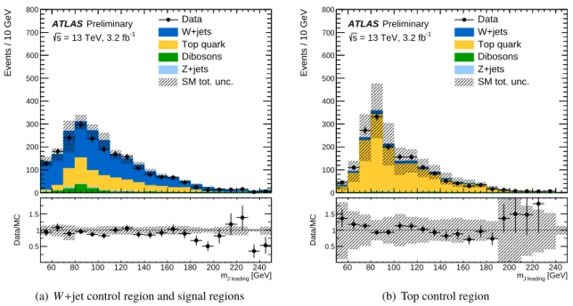
Figure 1 shows a comparison of the jet mass distribution of data and expected backgrounds when all the selection requirements, except for the jet mass requirement, are applied.
Studies using simulated events show that the dominant background in each of the signal regions are events from t¯ t production ( ∼ 30 %) and W +jets production ( ∼ 60 %). The signal acceptance times efficiency after all selection requirements varies between about 15% to around 25% for the W W /W Z resonances decaying to `ν q q ¯ final states with ` = e, µ , depending on the choices of the benchmark model and the resonance mass.
6 Background determination
The reconstructed W W/W Z invariant mass, m `νJ , is an observable used to search for a localized excess of events beyond the SM prediction. It is reconstructed on an event-by-event basis using the kinematic constraint m(`ν) = m(W ) that provides an estimate of the component of the neutrino momentum along the beam axis. The shapes from SM production of W /Z +jets, t t ¯ and single-top events are modeled using simulated events. Their normalizations are determined from a combined fit to the events in the signal and control regions. Since the background contribution from SM diboson production is very small, both its shape and normalization are taken from simulation. Its cross section is fixed to the value obtained by an inclusive next-to-leading order calculation with a 11 % systematical uncertainty assigned.
The contribution of multijet production to the selected samples originates from events where either another object is incorrectly identified as lepton, or a real but non-prompt lepton is produced in heavy flavor decays. The shapes of kinematic distributions in multijet background events are obtained from an independent data sample that satisfies the signal selection criteria except for the lepton requirement:
the electrons are required to satisfy a looser identification criterion (“MediumLH" but not meet the
“TightLH" selection criteria) and fail the isolation requirement; the selected muons are required to satisfy all the selection criteria but inverting the transverse impact parameter significance cut. The contributions of other processes with real leptons are subtracted from data using samples of simulated events in the extraction of the multijet background shape. The normalization of the multijet background is estimated by a fit to the transverse mass ( m T ) distribution of the leptonically decaying W candidates using data events in the signal region. The transverse mass is defined as m T = p
2 p T (`)p T (ν) · ( 1 − cos ∆φ `,ν ) ,
where ∆φ `,ν is the azimuthal angle between the lepton and the missing transverse momentum. In the fit,
the normalizations of the W /Z +jets and the multijet components are allowed to float, but all the other
backgrounds are taken from their respective predictions from simulation. The background contribution
from multijet production in the signal region is found to be negligible.
[GeV]
J leading
m
Events / 10 GeV
0 100 200 300 400 500 600 700 800
ATLAS Preliminary = 13 TeV, 3.2 fb -1
s
Data W+jets Top quark Dibosons Z+jets SM tot. unc.
[GeV]
J leading
m
60 80 100 120 140 160 180 200 220 240
Data/MC 0.5 1 1.5
(a) W +jet control region and signal regions
[GeV]
J leading
m
Events / 10 GeV
0 100 200 300 400 500 600 700 800
ATLAS Preliminary = 13 TeV, 3.2 fb -1
s
Data W+jets Top quark Dibosons Z+jets SM tot. unc.
[GeV]
J leading
m
60 80 100 120 140 160 180 200 220 240
Data/MC 0.5 1 1.5
(b) Top control region
Figure 1: The jet mass distribution for signal regions and W +jets control region (a) and Top control region (b). The events shown here are required to pass all selection requirements except the one on the jet mass. The hatched band represents the statistical and systematic uncertainties.
7 Systematic uncertainties
The main systematic uncertainties on the background estimate arise from the potential mismodeling of background components. An uncertainty on the shape of the W/Z +jets background is obtained by comparing the m `νJ shape in simulation and in data in the W +jets control region after the expected t t ¯ and diboson contributions are subtracted. The ratio is fitted with a first order polynomial and its deviation from unity is used as the W/Z+jets shape modeling uncertainty.
The data and simulation show a very good agreement for events in the top control region. The uncertainty in the shape of the m `ν J distribution from the t¯ t background is estimated by comparing a sample generated by the aMC@NLO [23] interfaced with Pythia 8.186 to the nominal sample. Additional systematic uncertainties are evaluated by comparing the nominal sample showered with Pythia to one showered with Herwig [47]. Samples of t t ¯ with the factorization and renormalization scales doubled and halved are compared to the nominal sample, and the largest difference observed is taken as an additional uncertainty.
Other systematic uncertainties such as on the small- R jet energy scale and resolution, trigger efficiencies, lepton reconstruction and identification efficiencies, lepton momentum scales and resolutions, b -tagging efficiency and misidentification rate, and missing transverse momentum are considered when evaluating possible systematic effects on the shape or normalization of the background estimation, as well as the shape and efficiency of the signal yield. They are found to have a minor impact on the analysis.
The large- R jet energy and mass scale uncertainties are evaluated with ATLAS Run 1 data, by comparing
the ratio of calorimeter-based to track-based measurements in dijet data and simulation [46], and are
validated by in-situ data of high- p T W boson production in semi-leptonic top pair events.
[GeV]
J l ν
m
1000 2000 3000
Normalized Events
10 -4
10 -3
10 -2
10 -1
1 10
NWA
LWA 5%, m = 1.4 TeV LWA 10%, m = 1.4 TeV LWA 15%, m = 1.4 TeV
=1, m = 1.4 TeV M
plRSG k/
=1, m = 1.4 TeV HVT Model A, g
vqq l ν WV → X →
Simulation ATLAS
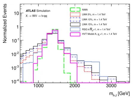
Figure 2: Reconstructed m `νJ distributions for different signal models.
The dominant uncertainties on the signal acceptance arise from the choice of PDF and from the uncertainty on the amount of initial and final state radiation present in simulated signal events. The PDF uncertainties are estimated by taking the acceptance difference between the NNPDF23LO and MSTW2008LO PDF and adding it in quadrature to the difference between the NNPDF23LO error sets.
The uncertainty on the integrated luminosity is 5 %. It is determined, following the same methodology as that detailed in Ref. [48], from a preliminary calibration of the luminosity scale using a pair of x − y beam-separation scans performed in June 2015.
8 Results
A simultaneous binned maximum-likelihood fit to m `νJ distributions of the events in the signal region, the top control region and the W +jets control region is performed using a statistical analysis package RooStats [49]. The fit includes five contributions: signal, W +jets, Z +jets, top and diboson. The W +jets and t¯ t normalizations are left free to float in the global fit while the diboson and Z +jets are constrained within their uncertainties, 11% [50] and 10% [51] respectively. The fit is performed simultaneously for the electron and muon channels. Systematic uncertainties are taken into account as nuisance parameters with Gaussian sampling distributions. For each source of systematic uncertainty, the correlations across bins and between different kinematic regions, as well as those between signal and background, are taken into account. Nineteen m `ν J bins between 500 and 3500 GeV are used in the fit with variable bin width in order to account for the expected resolution of a resonance peak as a function of the resonance mass while still keeping reasonably high statistics in each bin. The signal resonance distributions are shown in Figure 2.
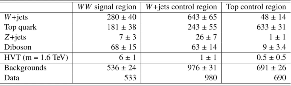
Tables 1 and 2 show the number of events predicted and observed in each region and when fitting to the
W W signal region and W Z signal region, respectively. The reconstructed m `νJ distributions for data and predicted background events as well as selected benchmark signal models in the signal and control regions are shown in Fig. 3. Good agreement is observed between the data and the background prediction.
Table 1: Event yields in W W signal and control regions for data and predicted background contributions after the fit. The expected yield for the HVT benchmark signal model are shown. Uncertainties are calculated after the fit to the data. The uncertainties on the total background correspond to the full statistical and systematic uncertainty.
W W signal region W +jets control region Top control region
W +jets 280 ± 40 643 ± 65 48 ± 14
Top quark 181 ± 38 243 ± 55 633 ± 31
Z +jets 7 ± 3 26 ± 7 1 ± 1
Diboson 68 ± 15 63 ± 14 9 ± 3.4
HVT (m = 1.6 TeV) 6 ± 1 1 ± 1 0.5 ± 0.5
Backgrounds 536 ± 24 976 ± 31 691 ± 26
Data 533 980 690
Table 2: Event yields in W Z signal and control regions for data and predicted background contributions after the fit.
The expected yield for the HVT benchmark signal model are shown. Uncertainties are calculated after the fit to the data. The uncertainties on the total background correspond to the full statistical and systematic uncertainty.
W Z signal region W +jets control region Top control region
W +jets 314 ± 52 655 ± 82 39 ± 18
Top quark 191 ± 43 270 ± 75 644 ± 32
Z +jets 5 ± 3 14 ± 5 1 ± 1
Diboson 55 ± 16 44 ± 11 7 ± 2.5
HVT (m = 1.6 TeV) 6 ± 1 1 ± 1 0.4 ± 0.1
Backgrounds 564 ± 34 983 ± 31 692 ± 26
Data 568 980 690
In the absence of a statistically significant excess in the data over the background prediction, the result is
used to evaluate an upper limit at the 95 % confidence level (CL) on the production cross section times
the branching fraction for various benchmark models. The exclusion limits are calculated with a modified
frequentist method [52], also known as CL s , and the profile-likelihood test statistic [53], using the binned
m `ν J distributions in signal and control regions. Systematic uncertainties and their correlations are taken
into account as nuisance parameters. None of the systematic uncertainties considered are significantly
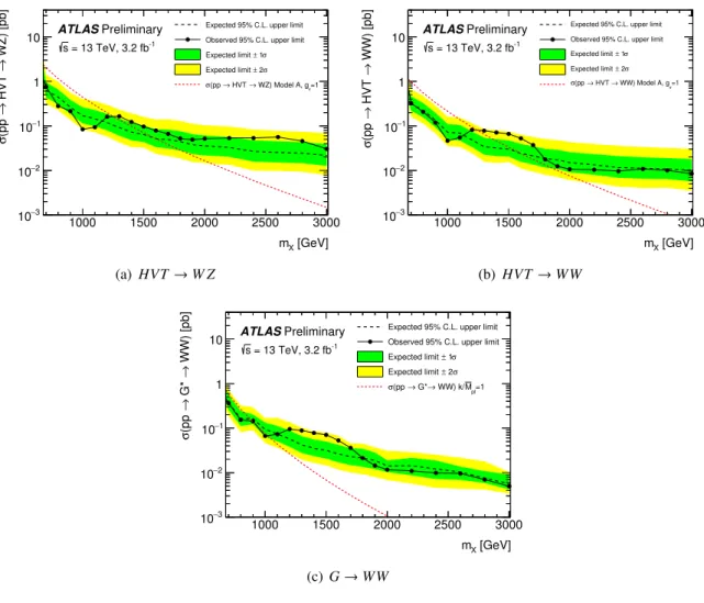
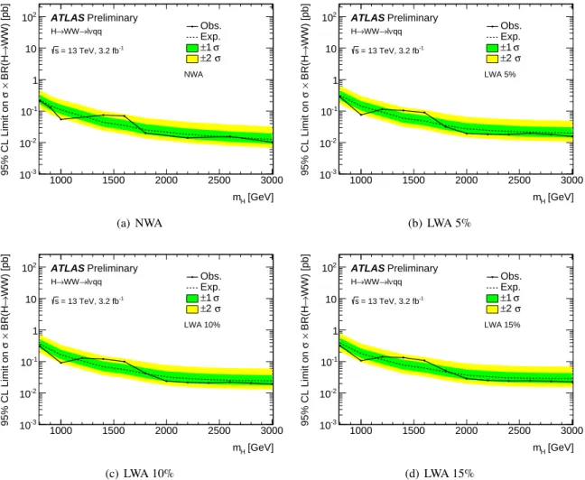
constrained or pulled in the likelihood fit. Figures 4 and 5 show the 95% CL upper limits on the production
cross section multiplied by the branching fraction into W Z and W W , as a function of the resonance mass,
for the HVT and heavy Higgs-like boson hypotheses respectively. For the Higgs-like boson the branching
ratios scale with m H as in the SM. A comparison of the result obtained with different widths is shown
Events / GeV
− 4
10
− 3
10
− 2
10
− 1
10 1 10 10 2
Data W+jets Top quark Dibosons Z+jets HVT m = 1.6 TeV Fit tot. unc.
ATLAS Preliminary = 13 TeV, 3.2 fb -1
s
WW Signal Region
[GeV]
m
lvJ500 1000 1500 2000 2500 3000
Data/MC 0.5 1 1.5
(a) W W Signal Region
Events / GeV
− 4
10
− 3
10
− 2
10
− 1
10 1 10 10 2
10 3
Data W+jets Top quark Dibosons Z+jets HVT m = 1.6 TeV Fit tot. unc.
ATLAS Preliminary = 13 TeV, 3.2 fb -1
s
WZ Signal Region
[GeV]
m
lvJ500 1000 1500 2000 2500 3000
Data/MC 0.5 1 1.5
(b) W Z Signal Region
Events / GeV
− 4
10
− 3
10
− 2
10
− 1
10 1 10 10 2
10 3 Data
W+jets Top quark Dibosons Z+jets HVT m = 1.6 TeV Fit tot. unc.
ATLAS Preliminary = 13 TeV, 3.2 fb -1
s
Top Control Region
[GeV]
m
lvJ500 1000 1500 2000 2500 3000
Data/MC 0.5 1 1.5
(c) Top Control Region
Events / GeV
− 4
10
− 3
10
− 2
10
− 1
10 1 10 10 2
Data W+jets Top quark Dibosons Z+jets HVT m = 1.6 TeV Fit tot. unc.
ATLAS Preliminary = 13 TeV, 3.2 fb -1
s
Hadronic W/Z sideband
[GeV]
m
lvJ500 1000 1500 2000 2500 3000
Data/MC 0.5 1 1.5
(d) W +jets Control Region
Figure 3: Reconstructed m `ν J distributions in data and the predicted background in the (a) W W signal region, (b)
W Z signal region, (c) top control region and (d) W +jets control region. The background expectation is shown after
the profile likelihood fit to the data. The band denotes the statistical and systematic uncertainty on the background
after the fit to the data. The lower panels show the ratio of data to the SM background estimate. The benchmark
model HVT with m = 1600 GeV is normalized to the expected cross section.
[GeV]
m X
1000 1500 2000 2500 3000
WZ) [pb] → HVT → (pp σ
3
10 − 2
10 − 1
10 −
1 10
Expected 95% C.L. upper limit Observed 95% C.L. upper limit
1σ Expected limit ±
2σ Expected limit ±
v=1 WZ) Model A, g HVT →
(pp → σ
ATLAS Preliminary = 13 TeV, 3.2 fb
-1s
(a) HVT → W Z
[GeV]
m X
1000 1500 2000 2500 3000
WW) [pb] → HVT → (pp σ
3
10 − 2
10 − 1
10 −
1 10
Expected 95% C.L. upper limit Observed 95% C.L. upper limit
1σ Expected limit ±
2σ Expected limit ±
v=1 WW) Model A, g HVT →
(pp → σ
ATLAS Preliminary = 13 TeV, 3.2 fb
-1s
(b) HVT → W W
[GeV]
m X
1000 1500 2000 2500 3000
WW) [pb] → G* → (pp σ
3
10 − 2
10 − 1
10 −
1 10
Expected 95% C.L. upper limit Observed 95% C.L. upper limit
1 σ Expected limit ±
2 σ Expected limit ±
pl