ATLAS-CONF-2010-062 28July2010
ATLAS NOTE
ATLAS-CONF-2010-062
July 21, 2010
A first measurement of the differential cross section for the J/ψ → µ+µ− resonance and the non-prompt to prompt J/ψ cross section ratio with pp
collisions at √
s = 7 TeV in ATLAS
The ATLAS Collaboration
Abstract
The inclusive production of the J/ψ meson in its dimuon decay mode is studied in proton-proton collisions at √
s =7 TeV with the ATLAS detector at the LHC. The double- differential cross section is measured with respect to the transverse momentum and rapidity ofJ/ψ. The ratio ofJ/ψmesons produced from B hadron decays to theJ/ψproduced from prompt QCD sources is also measured as a function ofJ/ψtransverse momentum.
1 Introduction
The mechanisms by which the production of prompt charmonium states take place in proton-proton collisions are not well understood. These processes comprise a good testing ground for a variety of QCD calculations. Various Tevatron measurements over the past few years have unveiled many interesting features of the dynamics of heavy quark production in high energy hadronic collisions ([1] and references therein). However, many questions still remain unanswered, and data obtained by the LHC collaborations should be able to shed new light on these processes in the new energy regime. This work begins in ATLAS with two measurements based on the resonance J/ψ→ µµ, which has a large production cross section and branching fraction into the easily accessible µ+µ− final state, making it a good target for study. Results are based on an integrated luminosity of up to 17.5 nb−1of LHC proton-proton collisions at 7 TeV.
Firstly we present a measurement of the production cross section of the J/ψ in bins of transverse momentum (pT) and rapidity (y). This is referred to in the note as thedifferential cross section.
Secondly, J/ψ are known to be produced in non-prompt mechanisms via the decay of long lived particles such asB-hadrons, and inpromptdecays from short-lived sources such as QCD-related subpro- cesses, and so we present a determination of the ratio
R ≡ dσ(pp→bbX¯ →J/ψX′) dσ(pp→J/ψX′′)prompt
(1) as a function of J/ψ pT, which is referred to as the “B → J/ψ ratio” or just the “ratio” in this note.
We use the notation B → J/ψto indicate that the source of the J/ψwas aB-hadron decay. This is an attractive measurement in the early data period, since the acceptances and efficiencies should be the same for the numerator and denominator.
The note is assembled as follows: in section 2 we give a brief overview of the ATLAS detector subsystems and triggers used in this analysis; in section 3 we describe the data samples used and the method by whichJ/ψ→µµcandidates are selected; in sections 4 and 5 we present the measurements of the differential cross section and the ratio respectively; and conclude in section 6.
2 Track and muon reconstruction in ATLAS
The ATLAS detector covers almost the full solid angle around the collision point with layers of tracking detectors, calorimeters and muon chambers. For the measurements presented in this paper the trigger system, the Inner Detector tracking devices (ID) and the Muon Spectrometer (MS) are of particular importance. The ATLAS coordinate system is described in the reference [2].
The Inner Detector has full coverage inφand covers the range|η|<2.5. It consists of a silicon Pixel Detector, a silicon strip detector (SCT) and a Transition Radiation Tracker (TRT). These detectors cover a sensitive radial distance from the interaction point of 50.5 mm up to 1066 mm and are immersed in a 2 Tesla axial magnetic field. The Inner Detector barrel (end-cap) parts consist of 3 (2x3) Pixel layers, 4 (2x9) layers of double-sided silicon strip modules, and 73 (2x160) layers of TRT straws.
The ATLAS Muon Spectrometer [2] designed to detect tracks over a wide region of|η|<2.7, consists of a large toroidal magnet (with an average magnetic field of 0.5 Tesla) and four detectors, each using a different technology. It has one Barrel Region (BR;|η| < 1.05) and two End-cap Regions (ER; 1.05 <
|η| < 2.7). Monitored Drift Tube chambers (MDT) in both the BR and ER sections and Cathode Strip Chambers (CSC) are used as precision chambers, whereas Resistive Plate Chambers (RPC) in the BR and Thin Gap Chambers (TGC) in the ER are used as trigger chambers. The chambers are arranged in three layers, so high-p particles traverse at least three stations with a lever arm of several metres.
The ATLAS detector has a three-level trigger system: Level 1 (L1), Level 2 (L2), and the Event Filter (EF). For these measurements, the trigger relies on the Minimum Bias Trigger Scintillators (MBTS), and/or the muon trigger chambers.
The MBTS are mounted at each end of the detector in front of the Liquid Argon Endcap-Calorimeter cryostats atz=±3.56 m and are segmented into eight sectors in azimuth and two rings in pseudorapidity (2.09 < |η| <2.82 and 2.82 < |η| <3.84). The MBTS trigger is configured to require two hits above threshold from either side of the detector. A dedicated muon trigger at the EF level is required to confirm the candidate events chosen for these measurements. This is initiated by the MBTS L1 trigger and searches for the presence of at least one muon track in the entire Muon Spectrometer (the full scan procedure). From now on we refer to this trigger as “the EF trigger”.
For the last period of runs analyzed in this note, the data were collected using either the EF trigger or the L1 muon trigger. The latter is based on two different trigger chambers: RPCs for the barrel region out to |η| < 1.05 and TGCs for the endcap region, 1.05< |η| < 2.4 [2]. It looks for hit coincidences within different RPC or TGC detector layers inside programmed geometrical windows which define the muon pT (L1 trigger roads), then selects muons above six programmable thresholds and provides a rough estimate of their positions, with coordinates ηandφ[3]. The muon trigger used for this analysis corresponds to the lowest pT threshold trigger which has a fully open road with a two-station time coincidence. No geometrical constraint (no road and then no pT selection) is applied. From now on we refer to this trigger as “the L1 muon trigger”.
Muon identification and reconstruction extends to|η| < 2.7, covering apT range from 1 GeV up to more than 1 TeV. In the muon reconstruction algorithms three categories of muons are foreseen:
• Muons from standalone reconstruction: thestandalonemuon reconstruction is entirely based on the tracks reconstructed in the Muon Spectrometer (MS). The track parameters are obtained from the MS track and are extrapolated to the interaction point, taking into account multiple scattering and energy loss in the traversed material. The standalone reconstruction covers|η|<2.7.
• Muons from combined reconstruction: thecombinedmuon reconstruction relies on a statistical combination of both a standalone MS track and an ID track, selecting the tracks to be paired on the basis of tight matching criteria to create a combined muon track. Due to ID coverage, the combined reconstruction covers|η|<2.5.
• Muons from ID track tagging: ataggedmuon is formed by segments which are not associated with an MS track, but which are matched to ID tracks extrapolated to the MS. Such a reconstructed muon adopts the measured parameters of the associated ID track. The muon tagging covers|η|<2 only.
In the current analysis, onlycombinedandtaggedmuons are used. Di-muon pairs with opposite charges were considered to be quarkonium candidates only if one of the two muons was combined (that is, tagged- tagged combinations are excluded except in the systematic studies). The inclusion of tagged-tagged combinations and their impact on the final result was used as a systematic check. In theJ/ψanalyses the muon track helix parameters are taken from the ID measurement alone since in this momentum range the contribution of the MS measurement does not improve the ID measurement.
3 Data and Monte Carlo samples
3.1 Data set
Collision data with a centre-of-mass energy of 7 TeV, taken between April 23rd and 4th June 2010, are included in this analysis. The analysis is based on data for which the beam and relevant apparatus have been declared to be stable.
Data are only included in this analysis if taken during stable beam LHC running, and in a period when the MS, ID and magnet systems were collecting data of a sufficiently high quality to be suitable for physics analysis.
3.2 Monte Carlo samples
Monte Carlo samples were generated using P 6 [4] tuned using the ATLAS MC09 tune [5] and MRST LO⋆[6] parton distribution functions, simulated with G4 [7] and fully reconstructed with the same software that was used to process the data from the detector. For the signal J/ψMonte Carlo (used for derivation of the kinematic acceptance corrections), we use P’s implementation of prompt J/ψ production subprocesses in the NRQCD Colour Octet Mechanism framework [8]. Prompt J/ψ production includes prompt production from the hard interaction, as well as radiative feed-down from χc → J/ψγdecays, which together we distinguish fromnon-promptproduction that is characterised by the production ofJ/ψvia the decay of aB-hadron.
The final results for the measured inclusive J/ψproduction cross-section and non-prompt to prompt production ratio are compared to P predictions at the generator-level. For the comparison, an ad- ditional Monte Carlo sample simulating the non-prompt contribution to J/ψ production was generated under the same conditions as that of prompt production, but using P’s minimum-bias process, which includes all basic parton-parton scattering subprocesses.
All samples were generated without polar or azimuthal anisotropy in the decay of theJ/ψ(the default in P), and reweighted at the particle-level to describe a number of different spin-alignment scenarios according to their respective angular dependencies (see Section 4.2 for more details), and these are then used to provide an uncertainty band on the final results, reflecting the theoretical uncertainty on the acceptance due to spin-alignment effects.
3.3 Event and candidate selection
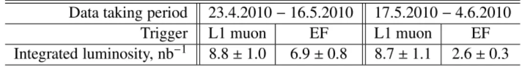
The data used in this analysis were taken during a period of LHC commissioning, so the instantaneous luminosity was rising from run to run. The analyses presented in this note deploy the two triggers described in section 2 - the EF trigger which is fed from the MBTS trigger, and the L1 muon trigger without an explicit pT threshold. The data sample is divided into an earlier (23rd April - 16th May) and a later (17th May - 4th June) sample. The EF trigger was prescaled towards the end of the first period with a factor of 2-4, while in the later period by factors of up to 10. The L1 muon trigger is not prescaled in either of the samples. Table 1 lists the integrated luminosity for each of the trigger selections used in the two data taking periods.
For the differential cross section measurement, in both periods, events are required to have passed the EF trigger. The efficiency of this trigger has been studied with data and is found to be close to 100% efficient for muons with pT greater than 4 GeV. The effective luminosity of the data used in the cross section measurement was 9.5 nb−1(see table 1). The ratio measurement is able to make use of an effective luminosity of 17.5 nb−1as trigger efficiencies play no role in the measurement.
To veto cosmic rays, events passing the trigger selection are required to have at least three tracks associated with the same reconstructed primary vertex. The three tracks must each have at least one hit in the pixel system and at least six hits in the SCT.
In each surviving event, pairs of reconstructed muons are sought. Only muons associated with ID tracks that have at least one hit in the pixels and six in the SCT are accepted. Muon pairs can be constructed from any combination of tagged and combined muons, as described in Section 2.
The two inner detector tracks from each pair of muons passing these selections are fitted to a common vertex [9]. No constraints on mass or pointing to the primary vertex are applied to the fit. Those
parameters after vertexing) of between 2 and 4 GeV, are regarded as J/ψ →µµcandidates. No further cuts are applied to the candidates.
Table 1:Integrated luminosities for samples used in these analyses
Data taking period 23.4.2010−16.5.2010 17.5.2010−4.6.2010
Trigger L1 muon EF L1 muon EF
Integrated luminosity, nb−1 8.8±1.0 6.9±0.8 8.7±1.1 2.6±0.3
4 Differential cross section of J/ψ → µ+µ− production
4.1 General considerations
The probability of a J/ψ →µ+µ−decay to be reconstructed depends on the kinematics of the decay, as well as muon reconstruction and trigger efficiencies. In order to recover the true number of such decays produced in the collisions, a weightwwas applied to each observedJ/ψcandidate, defined as the inverse of the above probability:
w−1 = A(pT, y, λi)× Eµ(~p1)× Eµ(~p2)× Etrig(~p1, ~p2) (2) where ~p1, ~p2 are the momenta of the two opposite-sign muons fromJ/ψ decay, while pT andyare the transverse momentum and rapidity of the J/ψ, and theλis represent the particular spin-alignment sce- nario. The muon reconstruction efficiency Eµ(~pi) is defined as the ratio of the number of reconstructed muons to the number of generated ones, in bins of muon transverse momentum,ηand φ. It was deter- mined from a high statistics sample of fully simulated promptJ/ψ →µ+µ−Monte Carlo events.
Only the EF trigger referred to in section 2 is used in the cross-section measurement. The efficiency of this muon triggerEtrig(~p1, ~p2) relative to the offline reconstruction was calculated using minimum bias data.
The kinematic acceptance A is defined as the probability that the decay of a J/ψ with transverse momentum pT and rapidityyhappens within the fiducial volume of the ATLAS detector. The latter is emulated by the generator-level cuts on momenta and pseudorapidities of the muons,|~p1|,|~p2|>3.5 GeV for|η1|,|η2|<2.0, and|~p1|,|~p2|>8.0 GeV for 2.0<|η1|,|η2|<2.5. These cuts eliminate the areas where the muon reconstruction efficiency is low.
The weight w defined in Equation 2 is applied to each J/ψ candidate which passes the selection criteria.
4.2 Acceptance correction
Determining the acceptance is of crucial importance for the cross section measurement, but unfortunately the spin-alignment (and therefore the angular distribution) of the J/ψ, which is not known under LHC conditions, may vary depending on the mechanism of production. As the acceptance depends on angular distributions, a complete measurement of the cross section cannot take place until the spin alignment is known. In this note we therefore perform the measurement under the assumption of a variety of spin alignment scenarios, and assign an appropriate systematic uncertainty.
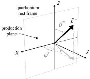
The acceptance A depends on five independent variables (two muon momenta constrained by the J/ψ mass condition), chosen as pT, y, azimuthal angle φ of J/ψ , and two angles characterising the J/ψ decay into two muons in its decay frame,θ⋆ andφ⋆. θ⋆ is the angle between the direction of the positive muon momentum in J/ψdecay frame, and the momentum of J/ψitself in the lab frame, while φ⋆ is defined as the angle between theJ/ψproduction and decay planes in the lab frame (see figure 1).
The distributions in θ⋆ andφ⋆ are different for various possible spin alignment scenarios of J/ψ . The coefficientsλθ, λφ, λθφin
d2N
dcosθ⋆dφ⋆ ∝1+λθcos2θ⋆+λφsin2θ⋆cos 2φ⋆+λθφsin 2θ⋆cosφ⋆ (3) are related to the spin density matrix elements of the J/ψspin wave function (see [10] and references therein):
|J/ψi=A−| −1i+A0|0i+A+|+1i (4) Five distinct spin alignment scenarios are considered in this study - a flat distribution, one longitudinal,
!
!
Figure 1: Definitions of theJ/ψpolarisation angles, in theJ/ψdecay frame.θ⋆is the angle between the direction of the positive muon in that frame, with respect to the direction of J/ψin the laboratory frame.
φ⋆is the angle between theJ/ψproduction plane and its decay plane. From [10].
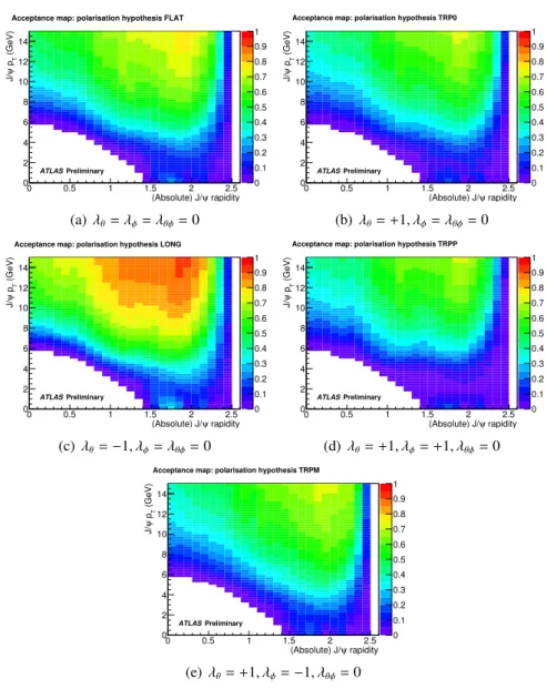
1. Flat distribution, independent ofθ⋆and φ⋆, i.e. λθ = λφ = λθφ = 0 labelled as “FLAT”. This is used as the main hypothesis.
2. Longitudinally alignedJ/ψdecays,A0 =1,A+= A−=0, yieldingλθ=−1, λφ=λθφ= 0 labelled as “LONG”.
3. Transversely aligned J/ψ decays, A+ = 1,A0 = A− = 0 or A− = 1,A+ = A0 = 0, yielding λθ= +1, λφ=λθφ=0 labelled as “TRP0”.
4. Transversely alignedJ/ψdecays,A+= A−,A0=0, yieldingλθ = +1, λφ= +1, λθφ=0 labelled as
“TRPP”.
5. Transversely aligned J/ψdecays, A+= −A−,A0 =0, yieldingλθ = +1, λφ =−1, λθφ =0 labelled as “TRPM”.
Two-dimensional acceptance maps are produced in bins of pT and y of J/ψ , for each of these five scenarios and are shown in Figure 2. The maps were obtained by reweighting the flat distribution at the truth level according to equation 3. The dependence of J/ψproduction on the azimuthal angleφis trivial and has been integrated out. In each of these scenarios we assume no explicit pT-dependence of the spin-alignment. It is certainly possible however for the average polarisation to vary as a function of quarkonium pT. These scenarios together map out an envelope in pT (and rapidity) of possible spin- alignment configurations and until explicitly measured is presented as a theoretical uncertainty around the final results.
rapidity (Absolute) J/ψ
0 0.5 1 1.5 2 2.5
(GeV)T pψJ/
0 2 4 6 8 10 12 14
0 0.1 0.2 0.3 0.4 0.5 0.6 0.7 0.8 0.9 1
ATLASPreliminary
Acceptance map: polarisation hypothesis FLAT
(a)λθ=λφ=λθφ=0
rapidity (Absolute) J/ψ
0 0.5 1 1.5 2 2.5
(GeV)T pψJ/
0 2 4 6 8 10 12 14
0 0.1 0.2 0.3 0.4 0.5 0.6 0.7 0.8 0.9 1
ATLASPreliminary
Acceptance map: polarisation hypothesis TRP0
(b) λθ= +1, λφ=λθφ=0
rapidity (Absolute) J/ψ
0 0.5 1 1.5 2 2.5
(GeV)T pψJ/
0 2 4 6 8 10 12 14
0 0.1 0.2 0.3 0.4 0.5 0.6 0.7 0.8 0.9 1
ATLASPreliminary
Acceptance map: polarisation hypothesis LONG
(c) λθ=−1, λφ=λθφ=0
rapidity (Absolute) J/ψ
0 0.5 1 1.5 2 2.5
(GeV)T pψJ/
0 2 4 6 8 10 12 14
0 0.1 0.2 0.3 0.4 0.5 0.6 0.7 0.8 0.9 1
ATLASPreliminary
Acceptance map: polarisation hypothesis TRPP
(d)λθ= +1, λφ= +1, λθφ=0
rapidity (Absolute) J/ψ
0 0.5 1 1.5 2 2.5
(GeV)T pψJ/
0 2 4 6 8 10 12 14
0 0.1 0.2 0.3 0.4 0.5 0.6 0.7 0.8 0.9 1
ATLASPreliminary
Acceptance map: polarisation hypothesis TRPM
(e) λθ= +1, λφ=−1, λθφ=0
Figure 2: Kinematic acceptance correction maps as a function ofJ/ψtransverse momentum and rapidity for specific spin-alignment scenarios considered in this note, that are representative of the extrema of possible polarisation configurations. Differences in acceptance behaviours particularly at low pT (where the bulk of the cross-section lies) occur between scenarios and can significantly influence the final result in a given bin.
4.3 Available phase space and binning
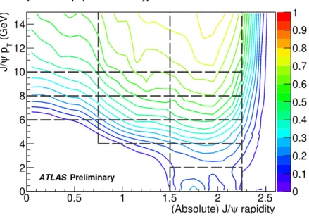
The acceptance map for spin alignment scenario 1 is shown in Figure 3 with the binning in J/ψ pT and rapidity overlaid.
rapidity (Absolute) J/ψ
0 0.5 1 1.5 2 2.5
(GeV) T pψJ/
0 2 4 6 8 10 12 14
0 0.1 0.2 0.3 0.4 0.5 0.6 0.7 0.8 0.9 1 Acceptance map: polarisation hypothesis FLAT
ATLASPreliminary
Figure 3: Kinematic acceptance correction map in J/ψ transverse momentum and rapidity showing equidistant contour lines (solid) of constant acceptance in the pT − y space, for the flat polarisation scenario native to the P Monte Carlo. Dashed lines are overlaid demarcating the bin boundaries used in this analysis.
In order to make sure that the available statistics are used efficiently, the rapidity interval is divided into three bins of equal width, 0−0.75,0.75−1.5,1.5−2.25, while the range of transverse momenta is split into six bins: 0−2,2−4,4 −6,6−8,8−10,10−15 GeV. Clearly, the measurement of the J/ψproduction cross section is only possible in those bins which are fully inside the acceptance of the ATLAS detector. The boundaries of these bins are highlighted in the figure by the dashed lines.
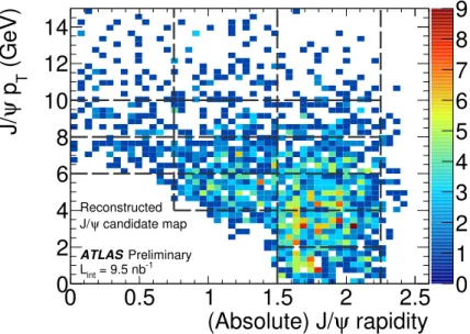
The distribution of reconstructed J/ψcandidates over the J/ψ pT −yplane is shown in Figure 4.3, with the pT, ybins used in this analysis marked by dashed lines. It can be seen that the majority ofJ/ψ candidates are reconstructed in low-pT, high-yareas, where the kinematic acceptance of ATLAS is fairly low (cf. Figure 3 above).
4.4 Muon reconstruction efficiencies
The muon reconstruction efficiency varies as a function of three variables, the transverse momentum pT, the pseudorapidityηand the azimuthal angleφof the track. Muon identification efficiency maps for com- bined and tagged muons are obtained from simulation using the samples of prompt pp → J/ψX →µµ production. The efficiency is calculated as the ratio of all reconstructed muons over the generated muons (combined and tagged separately); the following kinematic cuts were applied on the generated muons (as for the acceptance maps): momentum greater than 3.5 GeV for pseudorapidities less than 2.0, and momentum greater than 8 GeV for pseudorapidities between 2.0 and 2.5. These Monte Carlo results are validated with efficiency calculations from the data using the Tag and Probe method (which is currently limited by low statistics).
0 1 2 3 4 5 6 7 8 9
rapidity (Absolute) J/ψ
0 0.5 1 1.5 2 2.5
(GeV) T pψJ/
0 2 4 6 8 10 12 14
Reconstructed candidate map J/ψ
ATLASPreliminary = 9.5 nb-1
Lint
Figure 4: The distribution of reconstructed J/ψcandidates in the signal mass region (mJ/ψ±3σ) in pT and rapidity, overlaid with the bins used in the analysis separated by dashed lines.
4.5 Trigger efficiency
Using muons from minimum bias triggered data, the two-dimensional pT −ηmap of single muon ef- ficiencies for the EF trigger is constructed. From this map, the average efficiency for the EF trigger is calculated for each of the analysis bins by populating the bins with Monte Carlo prompt J/ψ → µ+µ− simulated events. The efficiency is found to be above 95% forJ/ψ pT greater than 6 GeV and drops to 57−63% for the lowestpT bins considered in this analysis.
The component of the weights (Equation 2) due to EF trigger efficiency is applied with appropriate systematic error, as follows:
• For regions of the map where the efficiency is approximately 50% (mainly the low pT bins), the weight is around 2 and we assign an error of±1 (i.e. 50%) to the weight
• Where the efficiency is approximately 80%, the weight is around 1.25 and we assign an error of
±0.25 (i.e.≈20%) to the weight
• Where the efficiency is close to 100% (all bins above 6 GeV) we do not assign an error.
In the lowerpT bins this assignment of systematic uncertainty is found to be more conservative than using the statistical variation of the efficiencies in each bin. It also avoids imposing an artificially large systematic error in the high pT bins where we know the trigger efficiency is very high, but where the statistics may be low and therefore have large fluctuations.
4.6 Fit of J/ψ mass distributions
For the differential cross section measurement the data in the (pT, y) bins described in the previous section are fitted as follows.
An unbinned maximum-likelihood fit is used to extract theJ/ψ mass and the number ofJ/ψ signal
candidates from the data. The log-likelihood function lnLis defined by:
lnL= XN
i=1
wi·lnh
fsignal(miµµ)+ fbkg(miµµ)i
(5) whereNis the total number of pairs of oppositely-charged muons in the invariant mass range 2<mµµ<
4 GeV.wi is the weight for theith event. The fsignal and fbkg represent the probability density functions that model the J/ψ signal and background mass shapes in this invariant mass range. Acceptance cor- rections A and efficiency corrections Eµ (described in previous sections) are applied for each event in turn.
For the signal, the invariant mass is modelled with a Gaussian distribution:
fsignal(mµµ, δmµµ)≡a0
√ 1
2πSδmµµ
e
−(mµµ−mJ/ψ)2
2(Sδmµµ)2 (6)
whose mean valuemJ/ψis theJ/ψ mass and its width is a productSδmµµ, and the overall multiplicative factor a0 is a free normalisation constant representing the fraction of invariant mass pairs in the mass region that are found in the J/ψ peak. The scale factor S is a free parameter of the fit and δmµµ is the measured mass error calculated for each muon pair from the covariance matrix associated with the di-muon vertex fit. For the background, the mass distribution is modelled with a linear function:
fbkg(mµµ)≡(1−a0)+b0mµµ (7) and b0 is a free parameter of the fit encapsulating the linear dependence of the background fit. The fit returns values of the free parameters a0,b0,mJ/ψ andS and a covariance matrix. They are used to calculate other characteristics of the data. The number of J/ψ signal decaysNsig and its uncertainty is calculated froma0and its uncertainty, and the total number of pairsN.
The mass resolutionσmis calculated by summing the result of the function fsignal(mµµ, δmµµ) over all candidates;σmdefines the region of the distribution for which the integral of sum over fsignal(mµµ, δmµµ) retains 68.27% of Nsig. The uncertainty onσmis calculated using the covariance matrices of the fitted vertices. The number of background events Nbck in the mass interval mJ/ψ ±3σm and its error are calculated froma0,b0,Nand the uncertainties ofa0,b0,mJ/ψandσm.
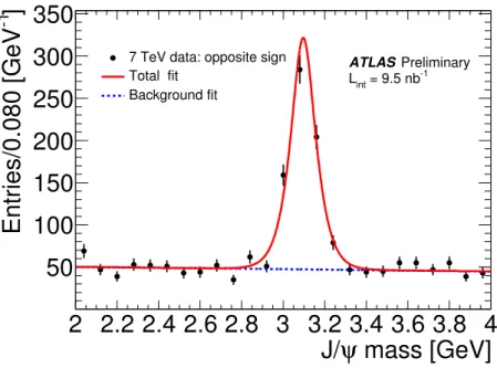
In Figure 5 the invariant mass for all oppositely charged muon pairs passing the selection for the differential cross section measurement (using the EF trigger only for both data taking periods), before acceptance and efficiency corrections, is shown. Overlaid on the figure are the background fit function and the combined background plus signal fit. TheJ/ψ mass returned by the fit is 3.096 GeV with an error of 0.003 GeV. The number ofJ/ψ signal events in the background subtracted peak isNsig=710±34, the mass resolution of the J/ψ signal isσm=0.070±0.003 GeV and the number of continuum background pairs in the mass range corresponding tomJ/ψ±3σmisNbck =373±10.
Various closure tests of the method described above are performed and the number of J/ψs in each bin is successfully recovered within expectations.
4.7 Results of the likelihood fits
In this section we present the invariant mass distributions of the selected candidate J/ψs for the inclusive differential cross-section. The invariant mass distributions forJ/ψ candidates before any corrections are shown in Figure 6 in the bins ofpTand|y|, defined previously. The maximum likelihood fitting procedure described in Section 4.6 is applied to these distributions and the fits are superimposed in figure 6.
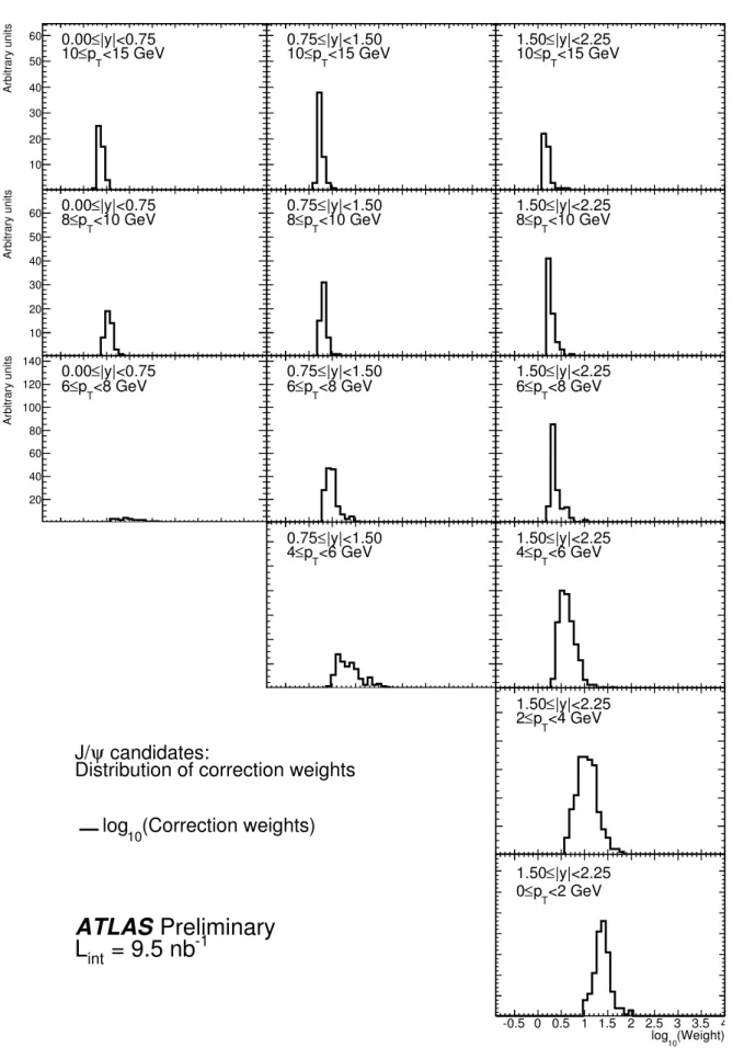
Figure 7 shows the distributions of the event-by-event weights (log10of the product of acceptance and efficiency corrections) derived according to the procedure explained previously. The average weights, along with those for each of the spin alignment scenarios, are shown in table 3.
mass [GeV]
J/ψ
2 2.2 2.4 2.6 2.8 3 3.2 3.4 3.6 3.8 4 ]-1 Entries/0.080 [GeV
50 100 150 200 250 300 350
7 TeV data: opposite sign Total fit
Background fit
ATLASPreliminary = 9.5 nb-1
Lint
Figure 5: Invariant mass distribution of reconstructed J/ψ →µ+µ−candidates used in the cross section analysis, corresponding to 9.5 nb−1. The points with error bars are data. The solid line is the result of maximum likelihood unbinned fit to all di-muon pairs in the mass window 2–4 GeV and the dashed line is the background fit result.
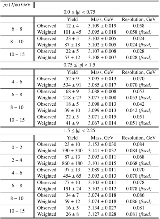
In figure 8 the same mass distributions are shown with the weights applied and the results of the new fits superimposed. Table 2 shows the number ofJ/ψcandidates under the peak (3σfrom the mean) before and after acceptance and efficiency corrections are applied. Additionally, table 2 shows the reconstructed fitted mass and width.
Table 2: J/ψcandidate yields before (top) and after (bottom) acceptance and efficiency corrections, in bins ofJ/ψtransverse momentum and rapidity. Errors are statistical only.
pT(J/ψ) GeV
0.0≤ |y|<0.75
Yield Mass, GeV Resolution, GeV
6−8 Observed 12±4 3.109±0.019 0.058
Weighted 101±45 3.095±0.018 0.058 (fixed) 8−10 Observed 23±5 3.102±0.005 0.024
Weighted 87±18 3.102±0.005 0.024 (fixed) 10−15 Observed 22±5 3.107±0.008 0.028
Weighted 53±12 3.108±0.007 0.028 (fixed) 0.75≤ |y|<1.5
Yield Mass, GeV Resolution, GeV
4−6 Observed 52±9 3.095±0.013 0.070
Weighted 534±91 3.085±0.017 0.070 (fixed)
6−8 Observed 68±9 3.088±0.008 0.053
Weighted 218±27 3.077±0.008 0.053 (fixed) 8−10 Observed 18±5 3.098±0.013 0.042
Weighted 39±10 3.099±0.013 0.042 (fixed) 10−15 Observed 22±5 3.071±0.015 0.051
Weighted 41±9 3.067±0.014 0.051 (fixed) 1.5≤ |y|<2.25
Yield Mass, GeV Resolution, GeV 0−2 Observed 23±10 3.153±0.030 0.084
Weighted 790±340 3.141±0.032 0.084 (fixed) 2−4 Observed 87±13 3.093±0.011 0.068
Weighted 860±180 3.101±0.015 0.068 (fixed) 4−6 Observed 97±13 3.089±0.011 0.070
Weighted 454±65 3.093±0.013 0.070 (fixed) 6−8 Observed 77±10 3.102±0.011 0.078
Weighted 191±24 3.102±0.012 0.078 (fixed) 8−10 Observed 34±7 3.074±0.018 0.086
Weighted 59±12 3.074±0.018 0.086 (fixed) 10−15 Observed 16±5 3.134±0.027 0.081
Weighted 26±8 3.127±0.028 0.081 (fixed)
2 2.2 2.4 2.6 2.8 3 3.2 3.4 3.6 3.8 4
Arbitrary units
0 5 10 15 20 25
30 0.00≤|y|<0.75
<15 GeV pT
10≤
2 2.2 2.4 2.6 2.8 3 3.2 3.4 3.6 3.8 4
Arbitrary units
0 5 10 15 20 25 30 35
40 0.00≤|y|<0.75
<10 GeV pT
8≤
2 2.2 2.4 2.6 2.8 3 3.2 3.4 3.6 3.8 4
Arbitrary units
0 10 20 30 40
50 0.00≤|y|<0.75
<8 GeV pT
6≤
2 2.2 2.4 2.6 2.8 3 3.2 3.4 3.6 3.8 4 0
5 10 15 20 25 30
<15 GeV pT
10≤≤|y|<1.50 0.75
2 2.2 2.4 2.6 2.8 3 3.2 3.4 3.6 3.8 4 0
5 10 15 20 25 30 35 40
<10 GeV pT
8≤ ≤|y|<1.50 0.75
2 2.2 2.4 2.6 2.8 3 3.2 3.4 3.6 3.8 4 0
10 20 30 40
50 <8 GeV
pT
6≤ ≤|y|<1.50 0.75
2 2.2 2.4 2.6 2.8 3 3.2 3.4 3.6 3.8 4 0
10 20 30 40 50 60 70
<6 GeV pT
4≤ ≤|y|<1.50 0.75
2 2.2 2.4 2.6 2.8 3 3.2 3.4 3.6 3.8 4 0
5 10 15 20 25 30
<15 GeV pT
10≤≤|y|<2.25 1.50
2 2.2 2.4 2.6 2.8 3 3.2 3.4 3.6 3.8 4 0
5 10 15 20 25 30 35 40
<10 GeV pT
8≤ ≤|y|<2.25 1.50
2 2.2 2.4 2.6 2.8 3 3.2 3.4 3.6 3.8 4 0
10 20 30 40
50 <8 GeV
pT
6≤ ≤|y|<2.25 1.50
2 2.2 2.4 2.6 2.8 3 3.2 3.4 3.6 3.8 4 0
10 20 30 40 50 60 70
<6 GeV pT
4≤ ≤|y|<2.25 1.50
2 2.2 2.4 2.6 2.8 3 3.2 3.4 3.6 3.8 4 0
10 20 30 40 50 60 70
<4 GeV pT
2≤ ≤|y|<2.25 1.50
Mass [GeV]
2 2.2 2.4 2.6 2.8 3 3.2 3.4 3.6 3.8 4 0
2 4 6 8 10 12 14 16 18 20
<2 GeV pT
0≤
|y|<2.25 1.50≤
candidates:
J/ψ
Unweighted invariant mass 7 TeV data: opposite sign Total fit
Background fit
ATLASPreliminary = 9.5 nb-1
Lint
-0.5 0 0.5 1 1.5 2 2.5 3 3.5 4
Arbitrary units
10 20 30 40 50
60 0.00≤|y|<0.75
<15 GeV pT
10≤
-0.5 0 0.5 1 1.5 2 2.5 3 3.5 4
Arbitrary units
10 20 30 40 50
60 0.00≤|y|<0.75
<10 GeV pT
8≤
-0.5 0 0.5 1 1.5 2 2.5 3 3.5 4
Arbitrary units
20 40 60 80 100 120
140 0.00≤|y|<0.75
<8 GeV pT
6≤
-0.5 0 0.5 1 1.5 2 2.5 3 3.5 4 10
20 30 40 50 60
<15 GeV pT
10≤≤|y|<1.50 0.75
-0.5 0 0.5 1 1.5 2 2.5 3 3.5 4 10
20 30 40 50
60 <10 GeV pT
8≤ ≤|y|<1.50 0.75
-0.5 0 0.5 1 1.5 2 2.5 3 3.5 4 20
40 60 80 100 120 140
<8 GeV pT
6≤ ≤|y|<1.50 0.75
-0.5 0 0.5 1 1.5 2 2.5 3 3.5 4 20
40 60 80 100
120 <6 GeV pT
4≤ ≤|y|<1.50 0.75
-0.5 0 0.5 1 1.5 2 2.5 3 3.5 4 10
20 30 40 50 60
<15 GeV pT
10≤≤|y|<2.25 1.50
-0.5 0 0.5 1 1.5 2 2.5 3 3.5 4 10
20 30 40 50
60 <10 GeV pT
8≤ ≤|y|<2.25 1.50
-0.5 0 0.5 1 1.5 2 2.5 3 3.5 4 20
40 60 80 100 120 140
<8 GeV pT
6≤ ≤|y|<2.25 1.50
-0.5 0 0.5 1 1.5 2 2.5 3 3.5 4 20
40 60 80 100
120 <6 GeV pT
4≤ ≤|y|<2.25 1.50
-0.5 0 0.5 1 1.5 2 2.5 3 3.5 4 20
40 60 80
100 <4 GeV pT
2≤ ≤|y|<2.25 1.50
(Weight) log10
-0.5 0 0.5 1 1.5 2 2.5 3 3.5 4 10
20 30 40 50 60 70
<2 GeV pT
0≤
|y|<2.25 1.50≤
candidates:
J/ψ
Distribution of correction weights (Correction weights) log10
ATLAS Preliminary = 9.5 nb-1
Lint
Figure 7: Distribution of the event-by-event correction weight (the product of acceptance and efficiency corrections) (log x-axis) applied to reconstructed J/ψ→µ+µ−candidates, split by transverse momen-