W bosonwiththeATLASdetectorattheLHC Measurementoftheproductioncrosssectionofheavyquarkjetsinassociationwitha Physik-Department

Physik-Department

Measurement of the production cross section of heavy quark jets in association with a W boson

with the ATLAS detector at the LHC

Dissertation von

Marco Vanadia

M¨ unchen

Juni 2013

TECHNISCHE UNIVERSIT ¨ AT M ¨ UNCHEN Max-Planck-Institut f¨ ur Physik

(Werner-Heisenberg-Institut)

Lehrstuhl f¨ ur Experimentalphysik

Measurement of the production cross section of heavy quark jets in association with a W boson

with the ATLAS detector at the LHC

Marco Vanadia

Vollst¨ andiger Abdruck der von der Fakult¨ at f¨ ur Physik der Technischen Universit¨ at M¨ unchen zur Erlangung des akademischen Grades eines

Doktors der Naturwissenschaften (Dr. rer. nat.) genehmigten Dissertation.

Vorsitzender: Univ-Prof. Dr. M. Beneke Pr¨ ufer der Dissertation:

1. Priv.-Doz. Dr. H. Kroha 2. Univ-Prof. Dr. L. Oberauer

Die Dissertation wurde am 05.06.2013 bei der Technischen Universit¨ at M¨ unchen einge-

reicht und durch die Fakult¨ at f¨ ur Physik am 12.06.2013 angenommen.

Abstract

In this thesis the production of a W boson in association with heavy-quark jets has been studied in proton-proton collisions at a centre-of-mass energy of 7 TeV with the ATLAS detector at the Large Hadron Collider (LHC).

For the identification of the W bosons and of the heavy quarks their semileptonic decays have been used. For this purpose, detailed studies of the muon reconstruction efficiencies of the ATLAS detector have been performed.

The associated production of a W boson with bottom quark jets represents an important background for searches for the Higgs boson and beyond Standard Model physics. It is therefore important to verify experimentally the Standard Model predictions for this process in the new energy regime of the LHC. The cross sections for W boson production together with a b-jet and zero or one additional jet have been measured for the first time at LHC energies and were found to be consistent with next-to-leading order QCD predictions.

The W boson production in association with a charm quark jet is of particular interest

because of the sensitivity to the strange quark content of the proton which is still rather

poorly constrained by experiments. The cross section measurements for this process in this

thesis are an important input for the determination of the strange quark parton density

function in the energy regime of the LHC.

Contents

Introduction 1

1 The Standard Model of Strong and Electroweak Interactions 3

1.1 Electroweak interactions . . . . 4

1.2 The Higgs mechanism . . . . 6

1.3 Quantum chromodynamics . . . . 7

1.4 Physics beyond the Standard Model . . . . 7

2 W and Z boson production at the LHC 9 2.1 Theoretical description of pp collisions . . . . 9

2.2 Overview of W

and Z boson production at colliders . . . . 11

2.3 Monte Carlo generators . . . . 13

3 The ATLAS experiment at the Large Hadron Collider 15 3.1 The Large Hadron Collider . . . . 15

3.2 The ATLAS detector . . . . 17

3.2.1 Notation and conventions . . . . 19

3.2.2 The Magnet System . . . . 19

3.2.3 The Inner Detector . . . . 20

3.2.3.1 The Pixel Detector . . . . 21

3.2.3.2 The Semiconductor Tracker . . . . 21

3.2.3.3 The Transition Radiation Tracker . . . . 21

3.2.4 The Calorimeter System . . . . 21

3.2.4.1 The Electromagnetic Calorimeter . . . . 22

3.2.4.2 The Hadron Calorimeter . . . . 23

3.2.5 The Muon Spectrometer . . . . 23

3.2.5.1 Monitored Drift Tube chambers . . . . 25

3.2.5.2 Cathode Strip Chambers . . . . 27

3.2.5.3 Alignment system for the precision chambers . . . . 28

3.2.5.4 Resistive Plate Chambers . . . . 28

3.2.5.5 Thin Gap Chambers . . . . 28

3.2.6 The Trigger System . . . . 29

iii

3.2.6.1 The first-level muon trigger system . . . . 29

3.2.7 Luminosity measurement in the ATLAS experiment . . . . 30

4 Reconstruction of physics objects 31 4.1 Detector simulation . . . . 31

4.2 Charged particle and vertex reconstruction in the Inner Detector . . . . 32

4.3 Electrons and Photons . . . . 33

4.3.1 Electron reconstruction . . . . 33

4.3.2 Photon reconstruction . . . . 34

4.4 Jets . . . . 35

4.4.1 Jet Reconstruction . . . . 35

4.4.2 Jet quality . . . . 36

4.4.3 Jet energy measurement . . . . 36

4.4.4 Heavy flavour jet tagging . . . . 37

4.4.4.1 The SV0 b-tagging algorithm . . . . 38

4.5 τ leptons . . . . 39

4.6 Transverse missing energy . . . . 39

4.7 Muons . . . . 39

4.8 Track and calorimeter isolation . . . . 42

5 Muon reconstruction performance 43 5.1 Measurement of the muon reconstruction efficiency . . . . 43

5.1.1 Dependence on the Muon Spectrometer regions . . . . 43

5.1.2 The Tag-and-Probe method . . . . 44

5.1.3 Data and Monte Carlo samples . . . . 45

5.1.4 Event selection . . . . 47

5.1.4.1 ID track quality cuts . . . . 47

5.1.4.2 Tag muon selection . . . . 48

5.1.4.3 Probe muon selection . . . . 48

5.1.4.4 Matching . . . . 51

5.1.5 Inner Detector reconstruction efficiency . . . . 51

5.1.6 Muon reconstruction efficiency . . . . 55

5.1.7 Systematic errors of the muon efficiency scale factors . . . . 57

5.1.8 Muon reconstruction efficiency for low-p

muons . . . . 59

5.2 Measurement of the muon trigger and isolation efficiency . . . . 60

5.3 Heavy flavour jet tagging efficiency . . . . 62

5.4 Conclusion . . . . 68

6 Measurement of the W + b-jet production cross section 69 6.1 Data samples used for the analysis . . . . 69

6.1.1 Overlap removal for the Alpgen W + jets samples . . . . 70

6.2 Event selection . . . . 72

Contents v

6.2.1 Preselection . . . . 72

6.2.2 Trigger requirements . . . . 72

6.2.3 Lepton selection . . . . 73

6.2.4 W boson selection . . . . 74

6.2.5 Jet selection and b-jet tagging . . . . 75

6.3 Background estimation . . . . 75

6.3.1 The W + jets background . . . . 75

6.3.2 The tt background . . . . 76

6.3.3 The QCD multi-jet background . . . . 78

6.3.3.1 Electron channel . . . . 78

6.3.3.2 Muon channel . . . . 78

6.3.3.3 QCD multi-jet m

templates . . . . 80

6.4 Cross section determination . . . . 80

6.5 Systematic uncertainties . . . . 83

6.6 Results of the fiducial cross section measurement . . . . 85

7 Measurement of the W + c-jet production cross section 89 7.1 Motivation . . . . 89

7.2 Measurement strategy . . . . 91

7.3 Samples used for the analysis . . . . 94

7.4 Event selection . . . . 95

7.4.1 Preselection . . . . 95

7.4.2 Trigger requirements . . . . 95

7.4.3 Lepton selection . . . . 96

7.4.3.1 Electron channel . . . . 96

7.4.3.2 Muon channel . . . . 96

7.4.3.3 Lepton-jet overlap removal . . . . 97

7.4.3.4 Lepton efficiency corrections . . . . 97

7.4.4 W boson selection . . . . 97

7.4.5 Jet selection . . . . 97

7.4.6 c-jet selection . . . . 98

7.5 Background estimation . . . . 99

7.5.1 QCD multi-jet background . . . . 99

7.5.1.1 Electron channel . . . 100

7.5.1.2 Muon channel . . . 101

7.5.2 W + light-jets background . . . 104

7.5.2.1 Electron channel . . . 104

7.5.2.2 Muon channel . . . 105

7.5.3 Refinement of the QCD multi-jet and W + light-jets background determination in the electron channel . . . 106

7.5.4 Z+ jets background . . . 107

7.6 Signal and background yields . . . 109

7.7 W

+ c-jet and W

+ c-jet production . . . 115

7.8 Yields as a function of the |η

| of the lepton from the W decay . . . 116

7.9 Cross section determination . . . 118

7.9.1 Determination of the selection efficiency . . . 119

7.9.2 Determination of the extrapolation factor . . . 120

7.9.3 c-hadron fragmentation and decay . . . 120

7.10 Measurement of the W

+ c-jet and W

+ c-jet production cross sections . 123 7.11 Systematic uncertainties . . . 124

7.11.1 Background estimation . . . 124

7.11.2 Detector effects . . . 126

7.11.3 Uncertainties in W + c signal modelling . . . 128

7.12 W + c-jet fiducial cross section results . . . 129

7.13 Combination of the electron and muon channels . . . 131

7.14 Comparison with theoretical predictions . . . 133

Conclusions 141

A Rejection of non-prompt muons 145

B Muon reconstruction performance in 2012 data 147

Bibliography 162

Acknowledgements 163

Nothing is insoluble. Nothing is hopeless.

Not while there’s life.

(Alan Moore, Watchmen)

Introduction

The Large Hadron Collider (LHC) at CERN is currently the largest particle accelerator in the world. Located near Geneva, in a 27.5 km long underground tunnel, after nearly two decades of planning and construction it started colliding protons steadily at a centre- of-mass energy of √

s=7 TeV since March 2010, an energy never reached before at particle colliders. In 2012 the centre-of-mass energy was raised to √

s=8 TeV. In early 2013 the LHC went into shutdown for upgrades to increase beam energy and instantaneous lumi- nosity. The LHC is the culmination of the physics experiments which tested and confirmed the Standard Model of particle physics in this and the last century shaping our knowledge of the most fundamental constituents of matters in the Universe.

The Standard Model is a theory of the electroweak and strong interactions between ele- mentary particles which has been developed to its present form in the 1960s and 70s, with quarks and leptons as fundamental constituents of matter and local gauge boson fields as mediator of the interactions. The Standard Model successfully describes the experimen- tal results obtained up to now and foreshadowed the existence of new phenomena and particles which were observed in the years following its formulation, as the the neutral weak current discovered with the Gargamelle bubble chamber at the CERN Proton Syn- chrotron and the W and Z bosons discovered by the UA1 and UA2 experiments at the CERN Super Proton Synchrotron. Many other experimental results in the last decades strengthened the Standard Model description and shaped our current knowledge of the fundamental constituents of matter with the discovery of new elementary particles: the charm quark (at the Stanford Linear Accelerator Center and at the Brookhaven National Laboratory), the bottom quark (by the E288 experiment at Fermilab), the τ lepton (at the Stanford Linear Accelerator Center), the gluons (at DESY laboratories), the top quark (by the CDF and D0 experiments at the proton-antiproton collider Tevatron at Fermilab) and the τ neutrino (by the DONUT experiment at the Tevatron).

The measurements performed by the experiments at the Tevatron and at the CERN Large Electron Positron (LEP) collider provided tests of the Standard Model with unprecedented precision. The last missing piece of the Standard Model was one of its cornerstones: the spinless Higgs boson which is related to the mechanism providing masses to the elementary particles without violating local gauge invariance. The search for this particle lasted for decades as the Standard Model makes no precise prediction for its mass.

1

Finally, on July 4

2012, the ATLAS and the CMS experiments at the LHC announced the discovery of a new particle with a mass of about 125 GeV/c

and the characteristics of the Higgs boson.

The experiments at the LHC test also other predictions of the Standard Model with high precision and at the highest energies reached by accelerators so far.

ATLAS is a general-purpose detector designed to study proton-proton interactions at the LHC with a very wide research program including Higgs boson searches, precision mea- surements of the strong and electroweak interactions, top quark physics, flavour physics, and searches for new physics beyond the Standard Model. In this thesis the cross sections for the production of a W boson in association with heavy charm and bottom quark jets predicted by the Standard Model has been measured with data collected by the ATLAS experiment in 2010 and 2011. These measurements probe the perturbative calculations and Monte Carlo descriptions of such processes, which are particularly relevant because these productions represent important background for many Standard Model and beyond Standard Model studies. Furthermore, the study of charm jets produced together with W bosons provide important information on the strange quark content of the proton which is currently known with high uncertainties.

In Chapter 1 a brief introduction to the Standard Model is given. Chapter 2 gives an overview of the phenomenology of weak boson production at the LHC with particular fo- cus on W + jets production. In Chapter 3 the LHC and the ATLAS detector are described, while in Chapter 4 an overview of the algorithms used for the evaluation of the trajectories and the energies of particles, hadron jets and other observables is given. Chapter 5 presents a detailed study of the performance of the ATLAS muon spectrometer and of the muon identification in data, which are important for the measurements presented in this thesis and for many other measurements by the ATLAS experiment involving muons. Chapter 6 describes the cross section measurement for the associated production of a W boson to- gether with at least one bottom quark jet using data collected in 2010 [1]. In Chapter 7 the cross section measurement using data collected in 2011 for the production of a W boson in association with a charm quark jet is explained [2]. Both cross section measurements have been produced by small analysis teams and are described in the respective chapters with particular focus on the major contribution of this work.

Conventions

Throughout the thesis, the International System of Units [3, 4] is used. The speed of light,

however, is fixed to c = 1. Thus, masses, momenta and energies are expressed in the same

units, namely the eV = 1.602176565(35) ·10

J. Charges are expressed in units of the

electron charge.

Chapter 1

The Standard Model of Strong and Electroweak Interactions

The Standard Model [5, 6, 7, 8] is our present best theory of the fundamental interactions intercurring between elementary particles. It is extremely successful in describing the experimental results of particle physics with high precision. Three of the four known interactions are described by the Standard Model (see Table 1.1):

ˆ the strong interaction responsible for the binding of quarks in hadrons and of the nucleons in nuclei,

ˆ the weak interaction responsible for instance for the radioactive β

decays,

ˆ and the electromagnetic interaction, responsible for the interactions between charged particles.

The Standard Model is a relativistic quantum field theory invariant under the local gauge transformation group

SU (3)

⊗ SU (2)

⊗ U (1)

(1.1)

with the SU (3)

symmetry group of the strong interaction and the SU (2)

⊗ U (1)

group describing the electroweak interactions. The Standard Model comprises 12 elemen- tary fermions, the gauge bosons of the SU (3)

⊗ SU (2)

⊗ U (1)

interactions between the fermions and the Higgs boson responsible for the SU (2)

⊗ U (1)

symmetry breaking which provides mass terms for the weak gauge bosons. These components are summarized in Table 1.2. All particles have a corresponding anti-particle with opposite charge and the same mass as a consequence of CPT invariance [9, 10, 11, 12].

The Standard Model particles are described by the following quantum fields:

ˆ Spinor fields Ψ for the fermions.

3

ˆ Vector gauge fields G

, B, W

for the gluons and the electroweak bosons.

ˆ The Scalar Higgs boson field Φ.

The brief review of the Standard Model presented in this chapter is based on [13, 14, 15].

Table 1.1:

Fundamental interactions

Interaction Range [m] Mediators Relative strength

Strong 10

gluons 1

Weak 10

W

and Z

bosons 10

Electromagnetic ∞ photon 10

Gravitational ∞ graviton (not discovered yet) 10

Table 1.2:

Elementary particles in the Standard Model Fermions (spin

/

) Bosons (spin 1) Boson (spin 0)

Quarks u c b W

Higgs boson

d s t Z

Leptons ν

ν

ν

γ

e µ τ gluons

1.1 Electroweak interactions

In the Standard Model, the electroweak interaction is described by the symmetry group

SU (2)

⊗ U (1)

. (1.2)

As introduced first by Glashow in 1961 [5], three conserved weak currents are related to the generators of the weak isospin group SU (2)

and one to the weak hypercharge group U (1)

. The observed charged weak currents can be identified as a combination of two SU(2)

currents, while the neutral weak and the electromagnetic currents are derived from a mixing of the SU (2) and U (1) currents.

The weak hypercharge Y is related to the electric charge Q and the third component of the weak isospin I by:

Y = 2(Q − I

) . (1.3)

The elementary fermions included in the Standard Model are arranged in weak isospin multiplets (see Table 1.3). The weak gauge bosons fields generated by the SU (2)

sym- metry group couple only with left-handed fermions, which are included in isospin doublets.

Right-handed leptons and quarks represent isospin singlets. Right-handed neutrinos would

be non-interacting particles and are therefore not included in the Standard Model.

1.1. Electroweak interactions 5

Table 1.3:

Quantum numbers of the elementary fermions in the Standard Model. The subscript

indicates left-handed particles, the subscript

indicates right-handed particles.

Fermions I I

Y Q

quarks

u d

L

c s

L

t b

L

1

/

/

/

/

/

-

/

/

-

/

u

c

t

0 0

/

/

d

s

b

0 0 -

/

-

/

leptons

ν

e

L

ν

µ

L

ν

τ

L

1

/

/

-

/

0

1

/

-

/

-

/

-1

e

µ

τ

0 0 -2 -1

The physical electroweak bosons fields W

, Z

, A are linear combinations of the fields corresponding to the generators of SU (2) and U (1), respectively the isospin triplet W

and the hypercharge singlet B

.

W

= 1

√

2 (W

∓ iW

), (1.4)

are the mediators of the charged weak interaction,

A

= B

cos(θ

) + W

sin(θ

), (1.5) is the photon field and

Z

= −B

sin(θ

) + W

cos(θ

) (1.6) the mediator of the neutral weak interaction. θ

is the Weinberg mixing angle [16].

This model describes the left-handed charged weak currents and the neutral weak and elec- tromagnetic currents interacting both with right-handed and left-handed fermions. The four gauge bosons are massless according to the local gauge symmetry of the interactions.

However, the W and Z bosons have experimentally observed masses needed to explain the

short range of the weak interactions. Explicit mass terms introduced into the Standard

Model Lagrangian would break the gauge invariance and thus the renormalizability of the

field theory.

1.2 The Higgs mechanism

The solution for this problem is provided by the Higgs mechanism [17, 18, 19, 20, 21, 22]

introduced into the Standard Model by Weinberg [6] and Salam [7] at the end of the 1960s.

The Higgs mechanism employs spontaneous symmetry breaking by introducing gauge bo- son masses. The Goldstone theorem [23, 24] states that the spontaneous breaking of a global continuous symmetry generates massless Goldstone bosons. The Higgs mechanism involves the spontaneous symmetry breaking of a local gauge symmetry, the SU (2)

⊗ U (1)

symmetry of the electroweak interaction.

A new contribution has to be included into the Lagrangian of the Standard Model:

L = (D

φ)

(D

φ) − µ

φ

φ − λ(φ

φ)

= (D

φ)

(D

φ) − V (φ) (1.7) with D

= ∂

+ igI · W

+ i

Y B

and g, g

being constants. This term describes the propagation and interaction field of a complex scalar weak isospin doublet field with Y = 1. Choosing a potential V (φ) with µ

< 0 and λ > 0 the ground state is not uniquely defined at |φ| = 0, but any state fulfilling the requirement

φ

φ = −µ

2λ ≡ v

2 . (1.8)

All ground states are connected by gauge transformations. An arbitrary ground state may be chosen, for instance φ

=

. The scalar Higgs field H(x) is a massive excitation from this ground state,

φ(x) = 1

√ 2

0 v+H(x)

, (1.9)

corresponding to a new neutral particle with mass m

= p

−2µ

. Massless excitations in the form of Goldstone bosons have been eliminated by gauge transformation into longitu- dinal polarization states of the W and Z

bosons. Inserting Eq. 1.9 into the Lagrangian of Eq. 1.7 the following expression is obtained:

L = 1

2 (∂

H)

− µ

H

+ g

v

4 W

W

+ v

(g

+ g

) 8 Z

Z

+ boson kinetic energy terms + higher order terms .

(1.10)

The spontaneously generated mass terms for the W

and Z bosons do not violate gauge

invariance and the photon remains massless. Mass terms for the fermions are also forbidden

by the global SU (2)

symmetry but can be generated preserving the gauge invariance by

introducing a new weak interaction between the fermions and the Higgs field.

1.3. Quantum chromodynamics 7

1.3 Quantum chromodynamics

The description of the strong interaction between quarks in the Standard Model is based on the SU (3)

symmetry group, where C stands for the colour charges of the gauge theory of the strong interaction which is therefore called quantum chromodynamics (QCD). The requirement of SU (3)

local gauge invariance of the Lagrangian of the quarks is satis- fied with the introduction of eight massless gauge bosons called gluons which mediate the strong interaction between coloured quarks. The non-Abelian structure of the symmetry group leads to self-interaction of the gluons which is responsible for the confinement of quarks and gluons in hadrons.

The difference between the photons, which are not electrically charged, and the weak and strong gauge bosons which carry the non-Abelian gauge charges is very important.

Vacuum polarization causes screening of the electric charge depending on the momentum transferred in the interaction, while the effect is reverted in the weak and the strong interactions. The electromagnetic coupling rises with decreasing distances, while the weak and the strong coupling decrease, an effect known as asymptotic freedom. Quarks in their bound states behave like free particles and perturbative QCD calculations are possible for high-energy processes. At large distances the coupling of the colour interaction becomes strong and perturbative calculations are no longer possible. Furthermore, when separating quarks at large distances, quark-antiquark pairs are created from the vacuum and form bound states with the original ones, a phenomenon called hadronization.

1.4 Physics beyond the Standard Model

While the Standard Model successfully describes essentially all experimental observations in the laboratory it leaves many questions unanswered. First of all it contains a large number of parameters which have to be experimentally determined. Extremely precise tuning of the parameters is needed to keep the mass of the Higgs boson at the low values predicted from the electroweak precision measurements at LEP and Tevatron and from the self-consistency of the theory. The Standard Model does not include a quantum theory of gravity, does not provide a description of dark matter and dark energy and cannot explain the observed asymmetry between matter and antimatter in the Universe.

Moreover the Standard Model has to be expanded to include neutrino masses for which there is experimental evidence from the observation of neutrino oscillations [25].

There are many extensions of the Standard Model addressing these and other open ques-

tions: Grand Unified Theories (GUT), supersimmetry (SUSY), string theory and many

others. To find hints for such new physics beyond the Standard Model is one of the many

goals of the experiments at the LHC.

Chapter 2

W and Z boson production at the LHC

In this chapter a short introduction to the phenomenology of proton-proton collisions will be given, with particular attention to the case of W

and Z

boson production. A brief overview of the Monte Carlo generators used to simulate the physics processes relevant for this thesis can be found at the end of the chapter.

2.1 Theoretical description of pp collisions

The composite nature of the proton is known since the 1950s [26]. According to the Stan- dard Model protons are bound states of two up and one down quark (valence quarks) which exchange gluons. In addition there are quark-antiquark pairs of any flavour which are generated from emitted gluons (sea quarks).

In the parton model the constituents of the proton are treated as free particles. Each parton carries a fraction x of the proton momentum. The different quark flavours and the gluons have different probabilities for carrying a certain momentum fraction in interactions with a given transferred momentum Q, which are described by the parton density functions (PDF) f (x, Q

). Knowledge of the PDFs is essential for a correct description of proton collisions. In Fig. 2.1 an evaluation of the PDF of the proton is shown: one can see that at high x values the dominant contributions are from the valence quarks, while at low x the gluon contribution dominates and the contributions from sea quarks become more relevant. This behaviour becomes more pronounced for high values of the transferred momentum. The s quark PDF is of particular interest for this thesis (see Chapter 7). In Fig. 2.1 it can be noticed that the predicted s quark contribution is lower compared to the one of the other light sea quarks u, d. The three distributions can be expected to be equal in the case of unbroken flavour symmetry. The different masses of the quarks leads to a suppression of the sea quark contributions increasing with the quark mass. The s quark PDF is currently poorly constrained by experimental data.

9

x 10-4 10^-3 10^-2 10^-1 1 )2xf(x,Q

0 0.2 0.4 0.6 0.8 1 1.2

g/10

d

d u

s u s, c c,

= 10 GeV2

Q2

x 10-4 10^-3 10^-2 10^-1 1 )2xf(x,Q

0 0.2 0.4 0.6 0.8 1 1.2

x 10-4 10^-3 10^-2 10^-1 1 )2xf(x,Q

0 0.2 0.4 0.6 0.8 1 1.2

g/10

d

d u

u s s, c c, b b,

GeV2

= 104

Q2

x 10-4 10^-3 10^-2 10^-1 1 )2xf(x,Q

0 0.2 0.4 0.6 0.8 1 1.2

MSTW 2008 NLO PDFs (68% C.L.)

Figure 2.1:

Parton distribution functions of the proton for momentum transfers squared of

= 10 GeV

and

= 10000 GeV

using the

parametrization [27].

Most physics analyses in proton-proton collisions are interested in the so-called hard pro- cesses, with high momentum transfer. In this case, the theoretical description is simpler, because at high energies the interaction between two constituents of the two colliding protons can be factorized and the remaining constituent particles can be considered as only spectators of this interaction. In Fig. 2.2 an example of a hard scattering process is given. The interacting quarks or gluons may radiate gluons or photons before the hard interaction producing initial state radiation (ISR). The same particles may be radiated by the final state particles produced in the interaction, a phenomenon known as final state radiation (FSR). The remnants of the protons may undergo soft interactions and may also radiate gluons and photons. All final state particles except the participants in the hard scattering process are called together the underlying event. The factorization between the hard interaction and the underlying event is an approximation. No coloured particles can be observed in the final state, due to the characteristics of the strong interaction discussed in Section 1.3, therefore coloured particles produced by the hard scattering must interact with coloured particles in the underlying event to result solely in colourless particles in the final state.

Assuming a generic interaction between two protons A and B and with a and b being the constituents of the protons participating in the hard interaction, the cross section of the overall process A + B → c + X, where c is the outcome of the hard scattering and X the proton remnants, can be expressed in terms of the elementary processes a + b → c by

σ

= X

a,b

Z

0

dx

Z

0

dx

[f

(x

, Q

)f

(x

, Q

)]σ

. (2.1)

The sum is over all the constituents a and b contributing to the production of c. f

and

2.2. Overview of W

and Z boson production at colliders 11

Interaction

ISR

FSR Incoming proton

Incoming proton

Proton remnant

Proton remnant

Interaction product

FSR Interaction product

Figure 2.2:

Illustration of a proton-proton collision with a hard scattering process between two constituents, a quark and a gluon, of the incoming protons. ISR stands for initial state radiation, FSR for final state radiation.

f

are the PDFs of the proton constituents.

2.2 Overview of W

and Z boson production at colliders

The experimental observation of the theoretically predicted W

and Z bosons was made in 1983 by the UA1 and UA2 collaborations in proton − anti-proton collisions at the the Super Proton Synchrotron (SPS) [28, 29, 30, 31]. The precision measurements of the Z bo- son mass were performed by the four experiments ALEPH, DELPHI, L3 and OPAL at the LEP collider [25]. At LEP-I, the Z bosons were produced in resonance at a centre-of- mass energy near the Z boson mass. The Z decay modes are into fermion − anti-fermion pairs with branching ratios (BR) shown in Table 2.1. The leptonic decays Z → e

e

and Z → µ

µ

provide a very clear signature for Z bosons production.

The W boson mass measurement is less precise due to the presence of neutrinos in the leptonic decay modes which cannot be detected. The most precise measurements are from LEP-II and from the CDF and D0 experiments at the Tevatron collider [25]. The main properties and decay modes of the W boson are listed in Table 2.1.

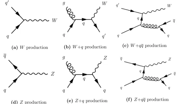
Figures 2.3a and 2.3d show the leading order (LO) Feynman diagrams for the W /Z pro- duction at hadron colliders. It is known since the end of the ’70s that LO computations are insufficient to describe these processes (see for example [32]). Currently complete next- to-next-to-leading order (NNLO) predictions are available for the inclusive production [33].

Final states with W /Z bosons associated with quarks and gluons are of particular inter-

est. Quarks and gluons in the final states produce cascades of particles which are observed

in the detectors as jets, i.e. as sprays of collimated particles. Figures 2.3b, 2.3c, 2.3e

Table 2.1:

Properties of the

and of the

bosons [25]. The

decays are charge conjugate to the ones of

.

Z

boson: m

= 91.1876 ± 0.0021 GeV; Γ

= 2.4952 ± 0.0023 GeV

Decay mode Branching ratio (%)

e

e

3.363 ± 0.004

µ

µ

3.366 ± 0.007

τ

τ

3.370 ± 0.008

invisible 20.00 ± 0.06

hadrons 69.91 ± 0.06

W

boson: m

= 80.385 ± 0.015 GeV; Γ

= 2.085 ± 0.042 GeV

Decay mode Branching ratio (%)

e

ν 10.75 ± 0.13

µ

ν 10.57 ± 0.15

τ

ν 11.25 ± 0.20

hadrons 67.70 ± 0.27

and 2.3f show the Feynman diagrams for the W /Z production in association with one or two final state quarks. Jets can also be originated by initial or final state radiation gluons in any of the diagrams of Figure 2.3. Next-to-leading order (NLO) perturbative QCD predictions for W +jets and Z +jets production have been developed in the last years, and experimental results are needed both to confirm these predictions and to provide input for further developments. These final states represent major backgrounds for many Standard Model and beyond Standard Model processes. An experimental determination of their cross sections and properties is crucial for a correct background estimation. These events provide also an insight on the proton content. Cross section measurements both of inclu- sive W /Z production and of specific W /Z+jets processes (for example W + c production which is the topic of Chapter 7) provide constraints on the proton PDFs. The strange quark PDF is of particular interest due to a tension between recent experimental results and the predictions [34].

The experimental results produced by the ATLAS and CMS collaborations at the LHC on W + jets [35, 36] and Z+ jets [36, 37, 38, 39] production are in general in good agree- ment with the predictions and show that LO multiparton event generators, normalised to NNLO cross section for the W inclusive production, describe the experimental data for all measured inclusive jet multiplicities within the estimated experimental and theoretical uncertainties. For W + jets production NLO calculations from MCFM [40], studied for events with at least two jets, and from Blackhat - Sherpa [41, 42], studied for events with at least four jets, were found to be mostly in agreement with the data [35].

Events with a vector boson produced in association with heavy-flavour quark jets, i.e.

bottom quark jets (b-jets) or charm quark jets (c-jets), represent a challenge for the exper-

2.3. Monte Carlo generators 13

iments due to their cross section, which is much smaller than the one of W /Z +light-jets (jets originated by u, d, s quarks or by gluons) production. In this thesis, in Chap- ters 6 and 7 cross section measurements for the production of a W boson in association respectively with b-jets and with one c-jet performed by the ATLAS collaboration are documented.

(a)W

production

+q production

+qq production

(d)Z

production

production

production

Figure 2.3:

Some of the lowest order Feynman diagrams for the

(+jets) and

tion in hadron collisions.

2.3 Monte Carlo generators

Monte Carlo simulations are of fundamental importance for most physics analyses as they provide the interface between theoretical expectations and experimental results. Simula- tions are used to estimate the backgrounds and to predict the signal strength as well as the event topologies, allowing for the optimisation of the signal selection criteria.

The generation of Monte Carlo events for a given process includes several steps: the

simulation of the hard scattering process according to calculated matrix elements (ME),

the propagation of the scattered partons into so-called parton showers (PS) under the

strong interaction, the formation of hadrons from the partons (hadronization) and finally

their decays into the final state particles. The emission of photons from particles in the

initial or final state is also simulated. For proton collisions the simulation of the underlying

event is additionally required. For most fundamental processes different Monte Carlo

generators can be used for different applications. The following generators have been used

in this thesis:

Pythia [43, 44]: a general-purpose leading order (LO) generator for particle collid- ers.

Herwig [45] and Herwig ++ [46]: a general-purpose LO generator, complementary to Pythia. The main differences between these two generators are in the description of the parton showering (PS) and fragmentation. Herwig++ is an improved version entirely written in the C++ programming language.

Alpgen [47]: a LO generator for Standard Model (SM) multi-parton processes at hadron colliders. It has to be interfaced with another program for PS and hadroniza- tion.

Sherpa [42]: a multi-parton LO generator which describes also the showering and the hadronization of the partons.

Blackhat [41]: generator specialised in next-to-leading order (NLO) calculations for W + jets and Z+ jets events; it can be interfaced with Sherpa.

Powheg [48]: a NLO generator of SM processes which needs to be interfaced with another program for PS and for hadronization.

MC @ NLO [49]: a NLO SM generator interfaced with Herwig / Herwig ++ for the parton showering.

aMC @ NLO [50]: an automated calculator for production processes at NLO which is interfaced with another program for PS and for hadronization.

AcerMC [51]: a generator of Standard Model background processes for top quark physics at the LHC.

EvtGen [52]: a generator dedicated to b-hadron physics.

Jimmy [53]: a Herwig based generator used for the simulation of the underlying event.

MCFM [40]: a parton-level generator used for the evaluation of NLO cross sections at hadron colliders.

A description of the simulation of the detector response to the generated particles will be

presented in Section 4.1.

Chapter 3

The ATLAS experiment at the Large Hadron Collider

The Large Hadron Collider (LHC) is a circular collider situated at CERN near Geneva in Switzerland [54]. Installed in the 26.7 km long tunnel previously occupied by the LEP collider [55], it is currently the world’s largest particle accelerator and the one with highest centre-of-mass energy. The physics program at the LHC started end of 2009. In the first two years it was operated at √

s = 7 TeV. The energy was raised to √

s = 8 TeV in 2012.

The LHC will be described in more detail in Section 3.1, followed by a description of the ATLAS experiment.

3.1 The Large Hadron Collider

The LHC is last in a chain of accelerators shown in Fig. 3.1. In this thesis the focus will be on proton-proton collisions, but the LHC is used as a lead-ion collider too. The use of hadrons in the collisions allows for high centre-of-mass energy, which by design can reach up to √

s = 14 TeV at the LHC. This is much higher than the energy reachable with a circular electron collider of the same size which is limited by synchrotron radiation. The composite nature of the protons is on the other hand challenging for the particle detectors at the LHC, as will be discussed in Section 3.2. The LHC has two independent vacuum pipes for the acceleration of the two particle beams crossing in four interaction points.

The LHC consists of 1232 super-conducting dipole magnets operating at 1.9 K with which magnetic fields up to 8.33 T strength can be achieved, necessary to keep the 7 TeV pro- ton beams on their orbits. The design parameters of the LHC machine are presented in Table 3.1, as well as the records reached by the LHC for those parameters in 2012 [56].

Fig. 3.1 shows the four interaction points where the main experiments are located.

ATLAS [57] and CMS [58] are general-purpose detectors designed to study Standard Model and beyond Standard Model physics processes at the highest energies achieved so far with the main focus on the Higgs boson search. LHCb [59] and ALICE [60] are detectors with

15

Figure 3.1:

The CERN accelerator complex.

specialized physics programs: LHCb is designed to study the b-hadron physics while AL- ICE studies the collisions of lead-ions.

Given a generic particle interaction physics process at a collider, the corresponding event rate in the experiments can be determined from the equation

dN

dt = Lσ( √

s) , (3.1)

where L is the instantaneous luminosity and σ( √

s) is the cross section of the process at the centre-of-mass energy √

s. In order to study challenging rare channels, the instantaneous luminosity L of the collider must be as high as possible. The luminosity depends on

Design parameters of the LHC [54] and achievements reached during 2012 as measured at the ATLAS interaction point [56]

Parameter Design Best achievement

Proton energy 7000 GeV 4000 GeV

Number of particles per bunch 1.15 · 10

1.66 · 10

Number of circulating bunches 2808 1380

Bunch crossing frequency 40 MHz 40 MHz

Bunch crossing time 25 ns 25 ns

Instantaneous Luminosity 10

cm

s

0.773 · 10

cm

s

3.2. The ATLAS detector 17

machine parameters. It can be expressed by the equation:

L = f nN

N

A , (3.2)

where f is the revolution frequency of the proton bunches in the collider, n the number of simultaneously circulating bunches, N

and N

the number of particles in each bunch and A is the cross section area of the colliding beams. The high number of bunches circulating in the LHC (see Table 3.1), resulting in a high frequency of bunch crossing, is meant for maximizing the luminosity.

3.2 The ATLAS detector

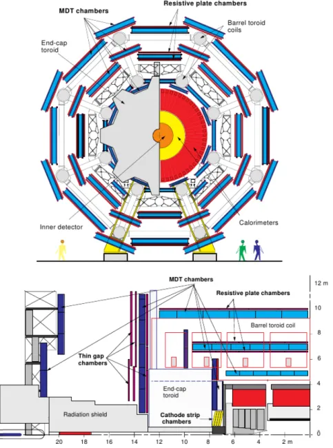
ATLAS [57] is one of the two main detectors at the LHC designed to study a wide range of particle physics processes at high energies. In this section the detector and its components are presented with emphasis on the performance goals that led its design. The detector is shown in Fig. 3.2.

Figure 3.2:

The ATLAS detector.

The characteristics of the LHC impose challenges to the experiments:

ˆ The high luminosity of the LHC leads to very high irradiation of the detector which

must have very high radiation resistance to guarantee the design performance over

several years of operation.

ˆ The high density of protons per bunch at the LHC leads to an high number of soft collisions happening in the same bunch crossing together with the hard process, the so-called “pile-up”. Detectors operating at the LHC must be able to identify and reconstructs particles and jets produced in hard scatterings which take place together with several tens of such soft collisions.

ˆ The high interaction rate and particle density produced in the collisions require fast and highly granulated detectors.

The physics goals of the ATLAS experiment lead to additional requirements on the detec- tor:

ˆ Precise reconstruction of the primary vertex of the hard interaction even at the high pile-up conditions.

ˆ A highly selective trigger system ensuring sufficient reduction of the data volume with still high efficiency for the interesting processes.

ˆ Efficient particle reconstruction and identification and a precise measurement of particle energies and of momenta.

ˆ Large solid angle coverage which is especially important for the reconstruction of processes involving neutrinos and other new weakly interacting particles which can only be observed by measuring the energy imbalance in the events.

ˆ Good energy resolution for electromagnetic showers in the calorimeters.

ATLAS consists of the following main elements:

ˆ The Magnet System, providing the magnetic field needed for the momentum mea- surement of particle tracks is introduced in Section 3.2.2.

ˆ The Inner Detector, a tracking system operating in a solenoidal magnetic field, is explained in Section 3.2.3.

ˆ The Calorimeter System used for the energy measurement of electromagnetically (electrons and photons) and strongly interacting particles is described in Section 3.2.4.

ˆ The Muon Spectrometer, operating in a toroidal magnetic field and designed to iden- tify muons and to measure their momentum is described in detail in Section 3.2.5 as this thesis is particularly concerned with the performance of the muon reconstruction in ATLAS.

ˆ The ATLAS Trigger System is described in Section 3.2.6.

ˆ The Luminosity Monitoring System providing the measurement of the luminosity

registered by ATLAS which is a key input for many physics analyses (see Sec-

tion 3.2.7).

3.2. The ATLAS detector 19

3.2.1 Notation and conventions

The coordinate system of ATLAS is defined in the following way (see [57]):

ˆ The origin is at the nominal interaction point.

ˆ The xy plane is transverse to the proton beams direction with:

– the y axis pointing upwards and

– the x axis pointing towards the centre of the LHC ring.

ˆ The z axis is oriented along the beam direction forming a right-handed coordinate system.

Other important variables are defined in the following way:

ˆ θ is the azimuthal angle measured from the z axis.

ˆ Pseudorapidity is defined as η= −ln(tan(

)).

ˆ φ is the polar angle in the xy plane.

ˆ Transverse momentum p

and transverse energy E

are defined in the xy plane, perpendicular to the beam axis.

ˆ Angular distance is measured by ∆R= p

∆η

+ ∆φ

.

Tracks are described by five parameters: cot(θ), φ, 1/p

, d

and z

. d

is the transverse impact parameter, the distance of closest approach from the beam axis in the xy plane.

z

is the longitudinal impact parameter, i.e. the z coordinate of the track at the point of closest approach to the interaction point. The detector hemispheres for z > 0 and z < 0 are defined as side A and side C, respectively.

3.2.2 The Magnet System

The ATLAS Magnet System [57] (see Fig. 3.2) consists of four superconducting magnets:

ˆ A central solenoid with a length of 5.3 m and a diameter of 2.6 m provides a 2 T magnetic field for the momentum measurement of charged particles tracks in the Inner Detector.

ˆ A toroidal air-core magnet system provides a bending power of R

Bdl =2-8 Tm for the muon spectrometer. It consists of a barrel and two endcaps magnets.

The barrel toroid consists of eight loops surrounding the calorimeters, with a length of

26 m and inner and outer diameters of 9.4 m and 20.1 m respectively. It covers the region

0 ≤ |η| ≤ 1.3 and provides a maximum field of 3.9 T. The endcap toroids are inserted into

the central one at the ends with a length of 5 m each, an outer diameter of 10.7 m and an inner diameter of 1.7 m. They cover the regions 1.6 ≤ |η| ≤ 2.7 and provide a maximum field of 4.1 T.

The bending power of the toroid system is reduced in the transition region between the barrel and the endcaps, for 1.3 < |η| < 1.6.

3.2.3 The Inner Detector

The Inner Detector (ID) [57], shown in Fig. 3.3, is a tracking system for charged particles in a solenoidal magnetic field. It consists of three sub-detectors:

ˆ the Pixel Detector,

ˆ the Semiconductor Tracker (SCT) and

ˆ the Transition Radiation Tracker (TRT).

The ID is 7 m long, has a diameter of 2.3 m, and covers the region 0 ≤ |η| ≤ 2.5. It has a very high granularity, especially close to the interaction region where precise secondary vertex reconstruction is needed for the identification of b-hadrons.

Figure 3.3:

The Inner Detector.

3.2. The ATLAS detector 21

3.2.3.1 The Pixel Detector

The Pixel detector consists of silicon pixel sensors and provides three precision position measurements along the track over the acceptance of 0 ≤ |η| ≤ 2.5. The barrel region of the detector consists of three detector layers at radii of 5 cm, 9 cm, 12 cm from the beam axis. The endcap regions consists of five disks each. The innermost layer (the B- layer) is most important for the decay vertex reconstruction and is also most affected by background radiation. The mechanical design of the detector allows for a substitution of the B-layer during the 2013-14 LHC shutdown period.

The Pixel Detector provides position measurements with excellent intrinsic resolution of 10 µm in the Rφ and of 115 µm in the Rz plane [61].

3.2.3.2 The Semiconductor Tracker

The Semiconductor Tracker (SCT) consists of four double layers of silicon strip detectors in the barrel and nine disk layers in the endcaps. In the barrel region the strips are oriented parallel to the beam direction while in the endcaps they are oriented radially.

The detectors provide position measurements with an intrinsic resolution of 17 µm in the Rφ plane and of 580 µm in the z direction in the barrel and in the radial direction for the endcaps [61], covering the region 0 ≤ |η| ≤ 2.5.

3.2.3.3 The Transition Radiation Tracker

The Transition Radiation Tracker (TRT) consists of a large number of straw drift tubes with a diameter of 4 mm assembled in 36 layers to provide on average 30 measurements per track in the region |η| ≤ 2.5. The straw tubes operate with a Xe (70%) CO

(20%) CF

(10%) gas mixture. The detector measures tracks in the Rφ plane with a single tube intrinsic resolution of 130 µm [61].

The TRT is also used for electron identification, especially at energies below 25 GeV. The use of a xenon gas mixture makes it possible to detect transition-radiation photons which are created in radiation sheets located between the straw tubes. The pion rejection factor varies between 20 and 100 depending on η [61].

3.2.4 The Calorimeter System

The Calorimeter System [57] provides energy and position measurements for electrons, photons and hadron jets. Furthermore it is essential for the reconstruction of hadronically decaying τ leptons and for the measurement of the missing energy via energy imbalance in the events, needed for the reconstruction of events with neutrinos or other weakly interacting particles (see Section 4.6).

The Calorimeter System consists of an Electromagnetic (EM) Calorimeter covering the

region |η| ≤ 3.2 and of an Hadronic Calorimeter (HCAL) covering |η| ≤4.9.

Figure 3.4:

The ATLAS Calorimeter System.

3.2.4.1 The Electromagnetic Calorimeter

The EM Calorimeter consists of a barrel part in the region |η| ≤ 1.475 and two endcaps for 1.375 ≤ |η| ≤ 3.2. It is a sampling calorimeter with Liquid Argon (LAr) as active medium in between accordion-shaped lead absorber plates. The region |η| ≤ 2.5 is used for precision measurements and is segmented into three longitudinal regions:

ˆ A pre-shower layer, with a thickness of about 6 radiation lengths (X

) and readout strips covering relative η angles between 0.003 and 0.25, depending on η itself, in order to provide a high granularity in η. The size of the segmentation of this layer is 0.1 in φ.

ˆ A middle section, with a thickness of about 16X

and a readout segmented into squares of ∆η × ∆φ = 0.025 × 0.025.

ˆ An outer layer, with an η depending thickness of 2-12X

and a readout granularity of ∆η × ∆φ = 0.050 × 0.025.

In addition in the region |η| < 1.8 a pre-sampling layer with a ∆η × ∆φ = 0.025 × 0.1

segmentation is used to estimate the energy loss of electrons and photons before the

calorimeters. In the region 2.5 < |η| ≤ 3.2 where electron and photon reconstruction

is not required, only two longitudinal samplings and a coarser granularity are sufficient to

3.2. The ATLAS detector 23

fulfil the required performance for jet energy and for energy imbalance measurements. In the region 3.1 ≤ |η| ≤ 4.9, the Forward Calorimeter (FCAL), which is also using LAr as active medium, provides both electromagnetic and hadronic shower measurements.

3.2.4.2 The Hadron Calorimeter

The Hadronic Calorimeter (HCAL) is a sampling calorimeter surrounding the EM Calorime- ter and covering |η| ≤ 4.9 . It is divided into the following regions:

ˆ The barrel HCAL for |η| ≤ 1.7.

ˆ Two endcap HCALs for 1.5 ≤ |η| ≤ 3.2.

ˆ The Forward Calorimeter (FCAL) covers the region 3.1 ≤ |η| ≤ 4.9.

The barrel HCAL uses iron as absorber and scintillating tiles as active material. The scintillation light is carried to photomultipliers by wave-length shifter (WLS) fibres. In the most part of the calorimeter the granularity is ∆η × ∆φ = 0.10 × 0.10.

The two endcap HCALs use LAr as active material and copper plates as absorber. They are divided into two wheels, the first one with 25 mm thick copper plates and the second one with 50 mm thick plates. The 8 mm wide gap between consecutive plates is equipped with three parallel electrodes, where the central one is the readout layer and the others carry the high voltage.

The FCAL works in a very high radiation environment which represents a challenge for the detector design. It uses LAr as active medium and copper and tungsten as absorber materials. The calorimeter consists of a metal matrix with longitudinal channels in which metal rods are inserted.

An important characteristics of the HCAL is its hermeticity. Its thickness is greater than 10 hadronic interaction lengths λ over the whole acceptance ensuring a good resolution for the jet energy and for the momentum imbalance measurements and low hadron punch- through into the muon system.

3.2.5 The Muon Spectrometer

The ATLAS Muon Spectrometer (MS) [57] is designed for the reconstruction of muons and the measurement of their momentum either as a stand-alone system or in combination with the Inner Detector. Due to the importance of muons for the analyses in this thesis, the MS design is discussed in detail below.

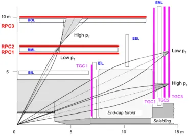
The Muon Spectrometer shown in Fig. 3.5 covers the region |η| ≤ 2.7 with a small gap at

|η| = 0 used for cables and services belonging to the Inner Detector and to the Calorimeter

systems. The following regions of the spectrometer can be distinguished:

ˆ The barrel region covering |η| ≤ 1.05 with the central region at |η| < 0.1.

ˆ The endcap regions covering 1.05 < |η| ≤ 2.7 with the transition regions between barrel and endcaps at 1.05 < |η| < 1.3 and the forward regions at |η| > 2.0.

The MS operates in the magnetic field of the toroid magnets described in Section 3.2.2.

The field bending plane is the Rη plane.

The MS uses four different types of muon chambers for muon reconstruction:

ˆ Monitored Drift Tube (MDT) chambers provide position measurement in the bend- ing plane over most of the MS acceptance region.

ˆ Cathode Strip Chambers (CSC) provide position measurement both in the bending and in the non-bending plane in the innermost detector layer of the forward regions.

ˆ Resistive Plate Chambers (RPC) are used for trigger information and for non- bending plane position measurement in the barrel region.

ˆ Thin Gap Chambers (TGC) are used for trigger information and non-bending plane position measurement in the endcap regions.

In the following the position in the bending plane will be referred to as the precision co- ordinate and the position in the non-bending plane as the transverse coordinate.

In the barrel region the precision MDT chambers are arranged in three layers with cylin- drical symmetry around the beam axis providing the three track position measurements needed for momentum determination:

ˆ The inner (I) layer at R=5 m.

ˆ The middle (M) layer at R=7.5 m.

ˆ The outer (O) layer at R=10 m.

In the endcaps chamber layers are located at 7 m (I), 14 m (M) and 21-23 m (O) from the nominal interaction point.

The chambers are arranged in polar octants, each divided into two sectors, one with larger chambers (large sector) and one with smaller chambers (small sector). The MS layout is shown in Fig. 3.5. The small and large chambers partially overlap to ensure full spatial coverage and allow for relative alignment with tracks.

The expected muon momentum resolution is shown in Fig. 3.6 as a function of the muon

transverse momentum p

. In the low and medium p

region, the multiple scattering and

3.2. The ATLAS detector 25

Figure 3.5:

Cross section views of the ATLAS Muon Spectrometer in the non-bending plane (top) and in the bending plane (bottom).

energy loss fluctuations dominate, while in the high p

region the chamber spatial resolu- tion and the alignment of the chambers are the main effects determining the momentum resolution.

3.2.5.1 Monitored Drift Tube chambers

Monitored Drift Tube (MDT) chambers provide precision position measurement in the

bending plane over most of the solid angle covered by the Muon Spectrometer. 1150

Figure 3.6:

Contributions to the muon momentum resolution of the ATLAS Muon Spectrometer as a function of the muon transverse momentum [61].

chambers are operating in the spectrometer.

A MDT chamber is composed of drift tubes, with a length of 1-6 m, organized in two multilayers separated by a spacer; each multilayer is composed of 3 or 4 layers of tubes (see Fig. 3.7).

The tubes are operated with Ar/CO

(93/7) gas at a pressure of 3 bar. The walls of the tubes are grounded. A voltage of 3080 V is applied to the central wire. In Fig. 3.7 an illustration of the operation mechanism of a drift tube is shown. When a charged particle is crossing the tube, it produces electron-ion pairs along its path (primary ionization).

The electric field inside the tube causes the electrons to drift to the wire. Close to the wire the ionization electrons are sufficiently accelerated to produce new electron-ion pairs in a so-called avalanche process (secondary ionization). The multiplication factor (gain) of the device, which depends on the voltage applied, on the gas pressure and on the tube diameter, has been chosen to be 2·10

, sufficiently low to prevent streamers and to avoid ageing of the drift tubes. The drift of the electrons to the wire and of the ions to the tube walls induces an electric signal on the wire. This signal is used to measure the electron drift time with respect to the time the muon passes the tube, i.e. the proton bunch crossing time corrected for the muon time of flight.

The drift time measurement is then converted into the distance of smallest approach of

3.2. The ATLAS detector 27

Figure 3.7:

Layout of a Monitored Drift Tube chamber (left) and working principle of a drift tube (right).

the muon trajectory to the wire using the r-t relation, which is specific for the gas mixture and is determined depending on temperature and magnetic field strength. The muon track is fitted to the corresponding drift circles. Further details about the muon reconstruction are given in Section 4.7.

3.2.5.2 Cathode Strip Chambers

Cathode Strip Chambers (CSC) are multi-wire proportional chambers with readout cath- ode strips parallel and orthogonal to the wires used in the innermost layer of the 2.0 ≤ |η| ≤ 2.7 region of the MS, where the high background radiation rate would degrade too much the performance of the MDT chambers. The layout of the CSC is shown in Fig. 3.8.

Figure 3.8:

Schematic layout of a Cathode Strip Chamber.

CSC chambers operate with a Ar/CO

/CF

(30/50/20) gas. The wires are at a potential

of 2600 V. Charged particle crossing a CSC plane generate ionization charges which are

multiplied by an avalanche process near the wires. The precision coordinate is determined

as the mean of the orthogonal strip cathode coordinates weighted by the charge signals induced on them, with a resolution of about 60 µm for a single CSC plane. Each chamber is composed of 4 planes. The transverse coordinate is measured with a resolution of about 5 mm by the cathode strips oriented parallel to the wires, which have larger pitch.

The CSC chambers are designed to operate with a background radiation level up to 1000 Hz/cm

, which is sufficient to cope with the working conditions of the inner part of the forward spectrometer region.

3.2.5.3 Alignment system for the precision chambers

MDT and CSC chambers are installed with millimetre precision, but their positions must be known with a relative accuracy of 30 µm in order to reach the muon momentum resolution. To achieve this, the following strategy is used:

ˆ Straight muon tracks are used to measure the relative chamber positions when the toroidal magnetic field is turned off.

ˆ An optical alignment monitoring system connects the chambers in projective towers with respect to the interaction point and allows for the measurement of their relative movements with micrometer precision.

Further information can be found in [62] and [63].

3.2.5.4 Resistive Plate Chambers

Resistive Plate Chambers (RPC) are composed of two independent detector layers, each providing two-dimensional coordinate measurements. The layers consists of two Bakelite plates of 2 mm thickness separated by a 12 mm wide gap. The readout is provided by η cathode strips for the bending plane measurement and by φ strips for the non-bending plane measurement. They operate with C

H

F

/C

H

(97/3).

RPCs have a typical spatial resolution of 1 cm. Their excellent time resolution of 1 ns allows for their use as muon trigger chambers in the barrel region with identification of the bunch crossing from which the muon originates. They are arranged in three layers, two of them below and above the middle MDT layer and the third one at the outer MDT layer (see Fig. 3.5).

The first and the second RPC layers from the beam pipe are used for low-p

muon triggers while the larger level arm between the middle and outer layers enables high p

triggers.

3.2.5.5 Thin Gap Chambers

Thin Gap Chambers (TGC) are multi-wire proportional chambers with anode wire pitch

larger than the anode-cathode distance which are operated in a CO

/C

H

gas mix-

ture. The wires provide the coordinate measurement in the bending direction while the