ATLAS NOTE ATLAS-CONF-2016-035

A TLAS-CONF-2016-035 19 July 2016

ATLAS NOTE

ATLAS-CONF-2016-035

19th July 2016

Jet mass reconstruction with the ATLAS Detector in early Run 2 data

The ATLAS Collaboration

Abstract

This note presents the details of the ATLAS jet mass reconstruction for groomed large- radius jets. The jet mass scale calibrations are determined from Monte Carlo simulation. An alternative jet mass definition that incorporates tracking information called the track-assisted jet mass is introduced and its performance is compared to the traditional calorimeter-based jet mass definition. Events enriched in boosted W, Z boson and top quark jets are used to directly compare the jet mass scale and jet mass resolution between data and simulation.

This in-situ technique is also extended to constrain the jet energy scale and resolution.

© 2016 CERN for the benefit of the ATLAS Collaboration.

Reproduction of this article or parts of it is allowed as specified in the CC-BY-4.0 license.

1 Introduction

Jets are collimated streams of particles resulting from the production of high energy quarks and gluons.

The distribution of energy inside a jet contains information about the initiating particle. When a massive particle such as a top quark or W/Z bosons is produced with significant Lorentz boost and decays into quarks, the entire hadronic decay may be captured inside a single jet. The mass of such jets (jet mass) is one of the most powerful tools for distinguishing massive particle decays from the continuum multijet background; therefore, it is critical to improve the reconstructed jet mass by reducing its resolution (JMR) and any associated systematic uncertainties.

This note documents the reconstruction of the jet mass with the ATLAS detector [1]. Two jet mass definitions are presented, each with strength in specific kinematic regimes. The baseline large-radius jet mass is constructed solely from calorimeter information via the constituents of a jet. A second definition augments the calorimeter information using finer granularity inputs from the tracking detector. Each of these jet mass definitions are described in more detail in Sec. 5, following background information on the ATLAS detector, simulated samples, and object reconstruction respectively in Sec. 2, 3, and 4. After introducing the various methods, their resolutions are quantitatively compared in simulation in Sec. 6 and their systematic uncertainties are documented in Sec. 7. In-situ studies of both jet mass definitions are presented in Sec. 8 and 9, including a measurement of the jet mass and energy scales and resolutions.

Methods for improving upon the jet mass definitions are documented in Sec. 10. The note ends with conclusions and future outlook in Sec. 11.

2 ATLAS detector

ATLAS is a multi-purpose particle detector with nearly 4π coverage in solid angle.1 A lead/liquid-argon sampling electromagnetic calorimeter is split into barrel (|η| < 1.5) and endcap (1.5 < |η| < 3.2) sec- tions. A steel / scintillating-tile hadronic calorimeter covers the barrel region (|η| < 1.7) and two endcap copper/liquid-argon sections extend to higher pseudo-rapidity (1.5 < |η| < 3.2). Finally, the forward region (3.1 < |η | < 4.9) is covered by a liquid-argon calorimeter with Cu (W) absorber in the electro- magnetic (hadronic) section.

Inside the calorimeters is a 2 T solenoid that surrounds an inner tracking detector which measures charged- particle trajectories covering a pseudorapidity range |η | < 2.5 with pixel and silicon microstrip detectors (SCT), and additionally covering the region |η | < 2.0 with a straw-tube transition radiation tracker (TRT).

Outside the calorimeter is a muon spectrometer: a system of detectors for triggering up to |η | < 2.4 and precision tracking chambers up to |η | < 2.7 inside a magnetic field supplied by three large superconduct- ing toroid magnets.

1

ATLAS uses a right-handed coordinate system with its origin at the nominal interaction point (IP) in the centre of the detector and the z-axis along the beam pipe. The x-axis points from the IP to the centre of the LHC ring, and the y-axis points upwards. Cylindrical coordinates (r, φ) are used in the transverse plane, φ being the azimuthal angle around the z-axis.

The pseudorapidity is defined in terms of the polar angle θ as η = − ln tan(θ/2). Angular distance is measured in units of

∆R = p

(∆η)

+ (∆φ)

.

3 Data and Simulated Samples

The 2015 LHC collision data used in later sections gave a mean number of additional proton-proton (pp) interactions per bunch crossing of approximately 14 and a bunch spacing of 25 ns. Following require- ments based on beam and detector conditions and data quality, the dataset corresponds to an integrated luminosity of 3.2 fb

.

Samples of Monte Carlo (MC) simulated events are used for studying the detector response of various mass reconstruction techniques as well as for comparisons with data. Table 1 summarizes the MC samples used for the studies in this note. More details about the t t ¯ and single top, W/Z + jets, and diboson simula- tion settings can be found in Ref. [2–5]. QCD multijets, simulated with P ythia 8, are used to derive the calibration factors for the jet mass scale and also to study the jet mass resolution over a wide kinematic range. The exotic production of W

and Z

bosons provides a copious source of simulated boosted W bosons, Z bosons and of top quarks respectively. The signal samples are produced with W

and Z

boson masses ranging from 400 to 5000 GeV. The MC samples are processed through the full ATLAS detector simulation [6] based on G eant 4 [7].

Process ME Generator ME Fragmentation UE Cross-section

PDF Tune Order

t t ¯ Powheg-Box v2 [8] CT10 [9] Pythia 6 [10] P2012 [11] NNLO+NNLL [12–17]

Single top Powheg-Box CT10 Pythia 6 P2012 NNLO+NNLL [18–20]

W/Z +jets Sherpa 2.1.1 [21] CT10 Sherpa Default NNLO [22]

Diboson Sherpa 2.1.1 CT10 Sherpa Default NLO

QCD multijets Pythia 8 [23] NNPDF23LO [24] Pythia 8 A14 [25] N/A

W

(→ W Z ) P ythia 8 NNPDF23LO P ythia 8 A14 N / A

Z

(→ t¯ t) Pythia 8 NNPDF23LO Pythia 8 A14 N/A

Table 1: Overview of the simulated samples.

4 Object Definitions

Large-radius jets are formed using F ast J et [26] implementation of the anti-k

jet algorithm [27] with distance parameter R = 1.0 and then trimmed [28] by re-clustering the constituents of the jet into subjets using the k

algorithm with distance parameter R

= 0.2 and removing any of these subjets with trans- verse momentum (p

) less than 5% of the original jet p

. Large-radius calorimeter jets are built from calorimeter-cell clusters calibrated to the hadronic scale using the local cell signal weighting (LCW) method [29]. The jet energy and pseudorapidity is then further calibrated to account for residual de- tector e ff ects using energy and pseudorapidity dependent calibration factors derived from simulation [30–

32]. The jet mass calibration is the final calibration step for large-radius calorimeter jets and it is de- scribed in Sec. 5. All large-radius calorimeter jets are required to have p

> 200 GeV with |η | < 2.0.

Detector-stable simulated particles (cτ > 10 mm), excluding muons and neutrinos, are used as inputs for particle-level truth jets. Small-radius jets 2 are formed from calorimeter cell-clusters at the electromag- netic (EM) scale and then corrected on average for the impact of pileup. These jets are then calibrated to the hadronic scale as described in Ref. [31]. A further calibration is applied to data in order to correct for di ff erences in the response measured using in-situ techniques.

2

Small-radius jets are clustered using the anti-k

jet algorithm with R = 0.4 distance parameter.

Large-radius calorimeter jets are identified as W / Z-jets (top-jets) if there is a truth W / Z-boson (top quark) associated to their untrimmed jet area using the ghost association method [33]. The W/Z-jets (top-jets) are studied in simulated samples of W

boson (Z

boson) events and they are required to have p

> 250 GeV (> 350 GeV).

Tracks are reconstructed in the inner detector using an iterative algorithm seeded on combinations of measurements from the silicon detectors and combining a combinatorial Kalman filter with a stringent ambiguity solver [34]. Reconstructed tracks are required to have transverse momentum of at least 400 MeV, |η | < 2.5, and have at least seven hits in the pixel and SCT detectors. Not more than one module with such hits is allowed to be shared between multiple tracks in the pixel or SCT detector. Further, the total number of holes3 is not allowed to exceed two per track, and not more than one in the pixel detector.

Additionally, the tracks must have been used in the fit of the primary vertex, or they were not used in any vertex fit. In the latter case, their absolute value of z

times sin θ must be less than 3 mm. z

is the di ff erence between the longitudinal position of the primary vertex and the longitudinal position of the track along the beam line at the point where d

, the transverse impact parameter calculated with respect to the measured beam line position, is measured. Tracks are associated to jets using the ghost association method.

5 Jet Mass Definitions and Calibration

5.1 Jet mass definitions

The calorimeter-based jet mass (m

) for a large-radius calorimeter jet J with calorimeter-cell cluster constituents i with energy E

, momentum ~ p

(| p ~

| = E

) is defined as:

m

= v u t 

 X

i∈J

E





2

−



 X

i∈J

~ p





2

. (1)

The angular spread in the decay products of a boosted massive particle scales as 1/p

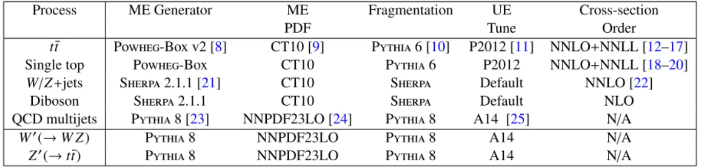
. For a su ffi ciently high Lorentz boost, this spread is comparable with the calorimeter granularity. Tracking information can be used to maintain performance beyond this granularity limit. One simple method for combining tracking and calorimeter information is the track-assisted jet mass (m

):

m

= p

p

× m

, (2)

where p

is the transverse momentum of a large-radius calorimeter jet, p

is the transverse mo- mentum of the four-vector sum of tracks associated to the large-radius calorimeter jet, and m

is the invariant mass of this four-vector sum (the track mass is set to m

). The ratio of p

to p

corrects for charged-to-neutral fluctuations, improving the resolution with respect to a track-only jet mass definition

3

Holes are defined as intersections of the reconstructed track trajectory with a sensitive detector element that do not result in a

hit.

(m

). This is illustrated by Fig. 1, which shows that the peak position and width of the track-assisted jet mass (dashed black line) are comparable to the calorimeter-based jet mass (dashed red line) and signi- ficantly better than the track-only jet mass (dashed blue line) for 1.6 TeV < p

< 1.8 TeV.

A procedure for correcting the jet mass as in Eq. 2 was first proposed using hadronic calorimetry to correct electromagnetic-only measurements [35, 36]. The extension to charged particle tracks was introduced in the context of top-quark jet tagging [37] using the HEPTopTagger algorithm [38, 39]. Since that time, there have been phenomenological studies using track-assisted jet mass4 for ultra boosted (p

&

O(10) TeV) boson and top quark jets [40, 41]. This note is the first experimental study of the track- assisted jet mass, including a discussion of its calibration and the associated systematic uncertainties.

Jet mass [GeV]

0 50 100 150 200

Fraction / 4 GeV

0 0.05 0.1 0.15 0.2 0.25

Simulation Preliminary ATLAS

= 13 TeV, W/Z-jets s

| < 0.4

< 1.8 TeV,|

1.6 TeV < p

m

m m

Uncalibrated Calibrated

Figure 1: Uncalibrated (dashed line) and calibrated (solid line) reconstructed jet mass distribution for calorimeter- based jet mass, m

(red), track-assisted jet mass m

(black) and the invariant mass of four-vector sum of tracks associated to the large-radius calorimeter jet m

(blue) for W / Z-jets.

5.2 Jet mass scale calibration

The jet mass scale (JMS) calibration procedure aims to correct, on average, the reconstructed jet mass to the particle-level jet mass by applying calibration factors derived from a sample of simulated QCD multijet events. The procedure is analogous to the jet energy scale (JES) calibration [30–32].

The calibration is derived using isolated large-radius calorimeter jets that are matched to isolated particle- level truth jets. A particle-level truth jet is considered matched to a large-radius calorimeter jet if it is within ∆R < 0.6 of the calorimeter jet. The isolation criteria is that there should be no other large-radius calorimeter (particle-level truth) jet with p

> 100 GeV within ∆R = 1.5 (2.5).

4

The phenomenological studies have not given a name to the quantity to Eq. 2, so it is defined here as the track-assisted jet

mass.

For each matched pair of large-radius calorimeter and truth jets, the jet mass response for a given jet mass definition is defined as:

R

= m

/m

; m

∈ c

· m

, c

· m

, (3) where c

is the jet energy scale calibration factor which depends on E

and η

. 5 The jet mass response is calculated using the reconstructed jet mass with the jet energy scale calibration applied. For each (p

, |η

|, m

)-bin, the average jet mass response hR

i is extracted and defined as the mean of a Gaussian fit to the jet mass response distribution. In order to be able to apply the calibration in data, the procedure must not depend on particle-level quantities. To this end, a numerical inversion technique is applied to calibrate a reconstructed jet quantity x

:

x

= x

hR

i ( f

( x

)) ≡ c

( E

or p

,η

, x

) · x

, (4) where f ( x) = hR

i(x ) · x, which is the average reconstructed jet quantity given the particle-level quantity and c

is the calibration factor for x

which is defined as the inverse of the average response (1/hR

i ).

In a given |η

|-bin, the jet mass scale calibration factors c

are parameterized as a function of p

and m

and the function is constructed by using a two dimensional Gaussian kernel (see Ref. [42] for more detail). For a reconstructed large-radius calorimeter jet with energy E

, reconstructed transverse momentum p

, detector pseudorapidity η

, calorimeter-based jet mass m

and track-assisted jet mass m

, the calibration is applied first for the jet energy and then for the jet mass:

m

= c

(c

· p

, |η

|, c

· m

) · c

· m

, (5) m

= c

(c

· p

, |η

|, c

· m

) · c

· m

, (6) where c

(c

) is the jet mass scale calibration factor for calorimeter-based (track-assisted) jet mass with a dependency on the JES-calibrated p

, |η

| and the JES-calibrated m

(m

). The jet mass is said to be calibrated if the average response hRi = 1 and the calibration procedure is deemed to fulfil closure when the same calibration factor is applied to the same sample from which it is derived.

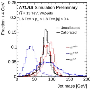
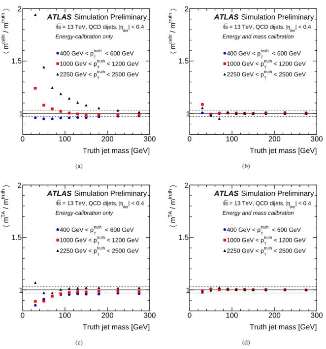
The jet energy calibration partially mitigates the inhomogeneities in the detector response as a function of η, but the full mass calibration is required to bring the average response close to one. Figure 2 (a, c) shows the calorimeter-based and track-assisted average jet mass response as a function of p

for several m

bins. Since the p

term in the definition of the track-assisted jet mass (Eq. 2) is calibrated, the residual jet mass calibration factors are smaller than for the calorimeter-based jet mass.

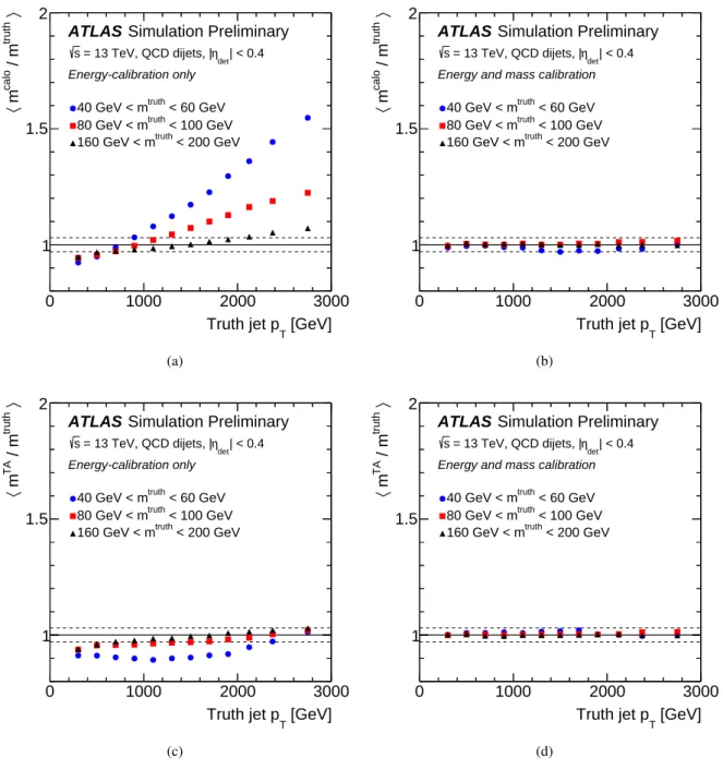
Figure 3 (a, c) shows the calorimeter-based and track-assisted average jet mass response for several |η

| bins. A dependency on |η

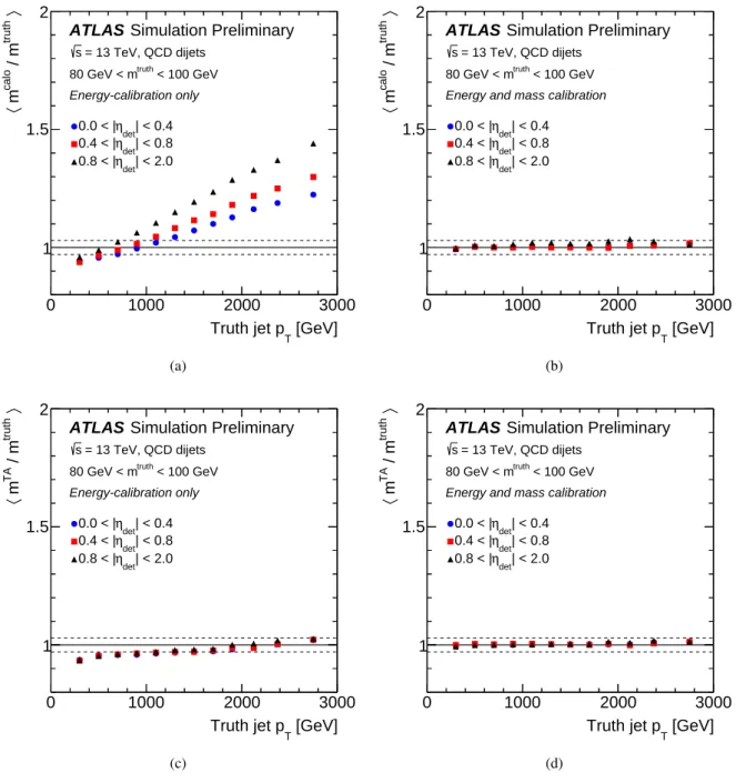
| is observed for the calorimeter-based average jet mass response while there is none for the track-assisted average jet mass response. Figure 4 (a, c) shows the dependency of both jet mass response on m

.

Following the jet mass scale calibration, a uniform jet mass response is restored to within about 3%

across the p

, m

and |η

| range for both reconstructed jet mass definitions as shown in Fig. 2 (b,

5

The pseudorapidity of the jet based on the detector geometry.

[GeV]

Truth jet p

0 1000 2000 3000

〉

/ m

m 〈

1 1.5 2

Simulation Preliminary ATLAS

| < 0.4 ηdet

= 13 TeV, QCD dijets, | s

Energy-calibration only

< 60 GeV

truth

40 GeV < m

< 100 GeV

truth

80 GeV < m

< 200 GeV

truth

160 GeV < m

(a)

[GeV]

Truth jet p

0 1000 2000 3000

〉

/ m

m 〈

1 1.5 2

Simulation Preliminary ATLAS

| < 0.4 ηdet

= 13 TeV, QCD dijets, | s

Energy and mass calibration

< 60 GeV

truth

40 GeV < m

< 100 GeV

truth

80 GeV < m

< 200 GeV

truth

160 GeV < m

(b)

[GeV]

Truth jet p

0 1000 2000 3000

〉

/ m

m 〈

1 1.5 2

Simulation Preliminary ATLAS

| < 0.4 ηdet

= 13 TeV, QCD dijets, | s

Energy-calibration only

< 60 GeV

truth

40 GeV < m

< 100 GeV

truth

80 GeV < m

< 200 GeV

truth

160 GeV < m

(c)

[GeV]

Truth jet p

0 1000 2000 3000

〉

/ m

m 〈

1 1.5 2

Simulation Preliminary ATLAS

| < 0.4 ηdet

= 13 TeV, QCD dijets, | s

Energy and mass calibration

< 60 GeV

truth

40 GeV < m

< 100 GeV

truth

80 GeV < m

< 200 GeV

truth

160 GeV < m

(d)

Figure 2: The average calorimeter-based jet mass response (a,b) and the average track-assisted jet mass response (c,d) as functions of p

for central jets in bins of m

before (a,c) and after (b,d) the mass calibration is applied.

The dashed lines are at 1 ± 0.03.

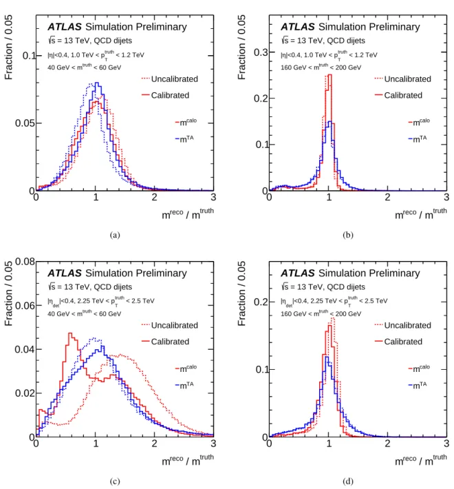
d), Fig. 3 (b, d) and Fig. 4 (b, d). For high p

and low m

jets, there is non-closure for the shape of the

calibrated calorimeter-based jet mass response distribution as shown in Fig. 5(c). The calorimeter-based

average jet mass response distribution does not retain the gaussian shape after the jet mass calibration is

applied. At low m

, the calorimeter-based average jet mass response decreases rapidly as a function

of m

, as shown in Fig. 4(a); therefore, in a fixed m

bin, lower mass response jets receive a larger

correction than higher mass response jets. The double-peak structure is additionally due to the large

[GeV]

Truth jet p

0 1000 2000 3000

〉

/ m

m 〈

1 1.5 2

Simulation Preliminary ATLAS

= 13 TeV, QCD dijets s

< 100 GeV

truth

80 GeV < m

Energy-calibration only

| < 0.4

0.0 < |

| < 0.8

0.4 < |

| < 2.0

0.8 < |

(a)

[GeV]

Truth jet p

0 1000 2000 3000

〉

/ m

m 〈

1 1.5 2

Simulation Preliminary ATLAS

= 13 TeV, QCD dijets s

< 100 GeV

truth

80 GeV < m

Energy and mass calibration

| < 0.4

0.0 < |

| < 0.8

0.4 < |

| < 2.0

0.8 < |

(b)

[GeV]

Truth jet p

0 1000 2000 3000

〉

/ m

m 〈

1 1.5 2

Simulation Preliminary ATLAS

= 13 TeV, QCD dijets s

< 100 GeV

truth

80 GeV < m

Energy-calibration only

| < 0.4

0.0 < |

| < 0.8

0.4 < |

| < 2.0

0.8 < |

(c)

[GeV]

Truth jet p

0 1000 2000 3000

〉

/ m

m 〈

1 1.5 2

Simulation Preliminary ATLAS

= 13 TeV, QCD dijets s

< 100 GeV

truth

80 GeV < m

Energy and mass calibration

| < 0.4

0.0 < |

| < 0.8

0.4 < |

| < 2.0

0.8 < |

(d)

Figure 3: The average calorimeter-based jet mass response (a,b) and the average track-assisted jet mass response (c,d) as functions of p

for jets with 80 GeV < m

< 100 GeV in bins of |η

| before (a,c) and after (b,d) the mass calibration is applied. The dashed lines are at 1 ± 0.03.

resolution of the jet mass so that in a fixed m

bin, there are two large populations of jets: those with

a low reconstructed mass that get a large correction (less than one) and those with a large reconstructed

mass that get a correction that is nearly unity (illustrated by Fig. 4(a)). For low p

jets (Fig. 5(a)) and

high m

jets (Fig. 5(b) and (d)), closure is observed for the shape of both jet mass response distributions

as the correction applied on the jet masses is small.

Truth jet mass [GeV]

0 100 200 300

〉

/ m

m 〈

1 1.5 2

Simulation Preliminary ATLAS

| < 0.4 ηdet

= 13 TeV, QCD dijets, | s

Energy-calibration only

< 600 GeV

truth

400 GeV < p

< 1200 GeV

truth

1000 GeV < p

< 2500 GeV

truth

2250 GeV < p

(a)

Truth jet mass [GeV]

0 100 200 300

〉

/ m

m 〈

1 1.5 2

Simulation Preliminary ATLAS

| < 0.4 ηdet

= 13 TeV, QCD dijets, | s

Energy and mass calibration

< 600 GeV

truth

400 GeV < p

< 1200 GeV

truth

1000 GeV < p

< 2500 GeV

truth

2250 GeV < p

(b)

Truth jet mass [GeV]

0 100 200 300

〉

/ m

m 〈

1 1.5 2

Simulation Preliminary ATLAS

| < 0.4 ηdet

= 13 TeV, QCD dijets, | s

Energy-calibration only

< 600 GeV

truth

400 GeV < p

< 1200 GeV

truth

1000 GeV < p

< 2500 GeV

truth

2250 GeV < p

(c)

Truth jet mass [GeV]

0 100 200 300

〉

/ m

m 〈

1 1.5 2

Simulation Preliminary ATLAS

| < 0.4 ηdet

= 13 TeV, QCD dijets, | s

Energy and mass calibration

< 600 GeV

truth

400 GeV < p

< 1200 GeV

truth

1000 GeV < p

< 2500 GeV

truth

2250 GeV < p

(d)

Figure 4: The average calorimeter-based jet mass response (a,b) and the average track-assisted jet mass response (c,d) as functions of m

for central jets in bins of p

before (a,c) and after (b,d) the mass calibration is applied.

The dashed lines are at 1 ± 0.03.

truth reco

/ m m

0 1 2 3

Fraction / 0.05

0 0.05 0.1

Simulation Preliminary ATLAS

= 13 TeV, QCD dijets s

< 60 GeV

truth

40 GeV < m

< 1.2 TeV

truth

|<0.4, 1.0 TeV < pT

η

|

m

m

Uncalibrated Calibrated

(a)

truth reco

/ m m

0 1 2 3

Fraction / 0.05

0 0.1 0.2 0.3

Simulation Preliminary ATLAS

= 13 TeV, QCD dijets s

< 200 GeV

truth

160 GeV < m

< 1.2 TeV

truth

|<0.4, 1.0 TeV < pT

η

|

m

m

Uncalibrated Calibrated

(b)

truth reco

/ m m

0 1 2 3

Fraction / 0.05

0 0.02 0.04 0.06 0.08

Simulation Preliminary ATLAS

= 13 TeV, QCD dijets s

< 60 GeV

truth

40 GeV < m

< 2.5 TeV

truth

|<0.4, 2.25 TeV < pT

ηdet

|

m

m

Uncalibrated Calibrated

(c)

truth reco

/ m m

0 1 2 3

Fraction / 0.05

0 0.1 0.2

Simulation Preliminary ATLAS

= 13 TeV, QCD dijets s

< 200 GeV

truth

160 GeV < m

< 2.5 TeV

truth

|<0.4, 2.25 TeV < pT

ηdet

|

m

m

Uncalibrated Calibrated

(d)

Figure 5: Uncalibrated (dashed line) and calibrated (solid line) jet mass response distributions for calorimeter-based jet mass (red) and track-assisted jet mass (blue) for central jets with 1.0 TeV < p

< 1.2 TeV (a,b) and 2.25 TeV <

p

< 2.5 TeV (c,d).

6 Jet Mass Performance in Simulation

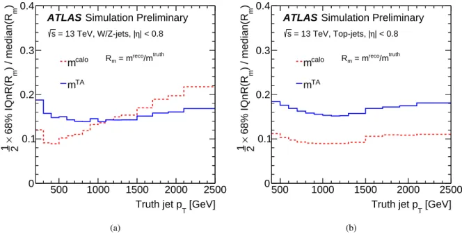
Figure 6 shows the jet mass resolution as a function of truth jet p

for W and Z bosons jets as well as top quark jets. There are many ways to quantify the resolution of the response distribution, but one robust method that is insensitive to outliers is to use half of the 68% interquantile range (IQnR)6 divided by the median. In the ideal Gaussian case, this quantity coincides with the standard deviation. The left plot in Fig. 6 shows that both the calorimeter-based and track-assisted jet mass resolution degrade at high p

; for the calorimeter this is due to finite granularity and for the tracker this is due to an increasing track resolution and an increased rate of track merging in the high density jet core. For W and Z boson jets, the track-assisted jet mass has a superior resolution to the calorimeter-based jet mass above about p

> 1 TeV. The charged-to-neutral fluctuations dominate the resolution of the track-assisted jet mass, which is worse than that of the calorimeter-based jet mass resolution below 1 TeV. In contrast, the track- assisted jet mass resolution is larger than the calorimeter-based jet mass resolution over the entire range p

range for top-quark jets. For a fixed p

, the separation between the decay products of primary particles with mass m is proportional to m. Therefore, the point at which the calorimeter granularity makes the calorimeter-based jet mass resolution worse than the track-assisted jet mass resolution is at a much higher p

. This point is also higher for top-quark jets due to the larger subjet multiplicity. The track-assisted jet mass performance can be improved at low p

by reducing the impact of charge-to-neutral fluctuations through local (subjet) corrections. This is explored in more detail in Sec. 10.2. The baseline track-assisted jet mass is most useful for W and Z boson jets with p

& 1 TeV, where the resolution is smaller than the calorimeter-based jet mass without any further modification.

[GeV]

Truth jet p

500 1000 1500 2000 2500

)

) / median(R

68% IQnR(R × 2 1

0 0.1 0.2 0.3 0.4

Simulation Preliminary ATLAS

| < 0.8

= 13 TeV, W/Z-jets, | s

truth reco

/m

m

= m

R

m m

(a)

[GeV]

Truth jet p

500 1000 1500 2000 2500

)

) / median(R

68% IQnR(R × 2 1

0 0.1 0.2 0.3 0.4

Simulation Preliminary ATLAS

| < 0.8

= 13 TeV, Top-jets, | s

truth reco

/m

m

= m

R

m m

(b)

Figure 6: The resolution of the jet mass response as a function of truth jet p

for W and Z boson jets (a) and top- quark jets (b) for calorimeter-based jet mass (red dashed line) and track-assisted jet mass (blue solid line). The half of the 68% interquantile range (IQnR) divided by the median of the jet mass response is used as an outlier insensitive measure of the resolution.

6

This is defined as q

− q

, whereby q

and q

are the 16

and 84

percentiles of a given distribution.

7 Jet Mass Systematic Uncertainties

A variety of methods are used to estimate potential sources of systematic differences in the jet mass scale and resolution between the data and simulation. Since the partonic center of mass energy is unknown at a hadron collider, there is no conservation law to use direct balance techniques to constrain the mass resolution using data, as it can be done for the jet p

. The jet mass scale of calorimeter-based jet mass is probed in the data by studying the ratio r

= m

/m

in an inclusive selection of high p

QCD dijet events [32]. The average value of r

is approximately 7 proportional to the jet mass scale and so 1 − hr

i

/hr

i

is a measure of the scale uncertainty. Track modeling and fragmentation modeling can also introduce changes in 1 − hr

i

/hr

i

, so their uncertainties limit the precision of this method to ∼ 5%. The r

-method cannot be used to measure the jet mass resolution because the resolution of r

is dominated by charged-to-neutral fluctuations. Instead, an in-situ method based on the hadronic-decay of W bosons and top quarks is used for this purpose, described in Sec. 9 in more detail.

One key advantage of the track-assisted jet mass over the calorimeter-based jet mass is that the systematic uncertainties can be determined through auxiliary studies. In particular, the jet mass scale and jet mass resolution uncertainty on m

are estimated by propagating the track reconstruction uncertainties and calorimeter-jet p

uncertainties through the definition in Eq. 2. The calorimeter-jet p

uncertainty is estimated using the p

version of the r

method: r

= p

/p

, though in the future any of the in-situ methods for small-radius jets could be adapted for this purpose.

The dominating track reconstruction ine ffi ciency for isolated particles is due to hadronic interactions with the inner detector material. Inside the core of high p

jets, an additional ine ffi ciency due to the high particle-density exists. For isolated tracks, the reconstruction efficiency uncertainty is estimated by vary- ing the amount of inner detector material within its measured uncertainty [43]. The uncertainty on the loss of tracks in the core of high p

jets is estimated with a data-driven technique based on the meas- ured energy loss of charged particles in the pixel detector [44]. In addition to the track reconstruction e ffi ciency, the other leading source of uncertainty is due to fake tracks resulting from badly reconstructed tracks. The modeling of fake tracks is probed in data by studying the pileup dependence of the number of reconstructed tracks. Based on the assumption that this dependency should be linear without any fake track contribution, the fraction of fakes is estimated by any observed non-linearity. A 30% uncertainty on the fake rate is assigned based on data / MC comparisons of this dependence. Furthermore, possible e ff ects due to the uncertainty in the reconstructed momentum of tracks were assessed using an iterative method based on Z → µµ events [45–47]. In addition to detector-based uncertainties, the modeling of frag- mentation leads to an uncertainty in the track-assisted jet mass resolution. A fragmentation uncertainty is estimated by comparing Pythia 8 and Herwig++.

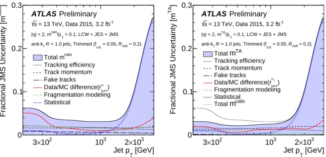
Figure 7 summarizes the various components of both the calorimeter-based and track-assisted jet mass scale uncertainties. The tracking uncertainties for m

and for m

(through r

) are fully correlated.

However, the impact of the tracking uncertainties are smaller for m

compared with m

because a large extent of the uncertainty cancels in the ratio m

/p

. At high p

, the uncertainty is limited by the size of the dataset used to assess the modeling of r

. Between about p

= 300 GeV and p

= 1 TeV, the uncertainty is about 4% for m

and about 2% for m

.

7

One can decompose r

= R × (m

/m

) × (m

/m

). If all three terms on the right hand side of

the equation are independent, then hr

i ∝ hRi. However, since the calorimeter response depends on the charged-to-neutral

ratio, this factorization is only approximate.

[GeV]

Jet p

10

×

3 10

2 × 10

]

Fractional JMS Uncertainty [m

0 0.1 0.2 0.3

Preliminary ATLAS

= 13 TeV, Data 2015, 3.2 fb-1

s

= 0.1, LCW + JES + JMS /pT

| < 2, mcalo

η

|

= 0.2) Rsub

= 0.05, = 1.0 jets, Trimmed (fcut tR

anti-k

Total m

Tracking efficiency Track momentum Fake tracks

m

)

track

Data/MC difference(r Fragmentation modeling Statistical

[GeV]

Jet p

10

×

3 10

2 × 10

]

Fractional JMS Uncertainty [m

0 0.1 0.2 0.3

Preliminary ATLAS

= 13 TeV, Data 2015, 3.2 fb-1

s

= 0.1, LCW + JES + JMS /pT

| < 2, mTA

η

|

= 0.2) Rsub

= 0.05, = 1.0 jets, Trimmed (fcut tR

anti-k

m

Total

Tracking efficiency Track momentum Fake tracks

T

)

p track

Data/MC difference(r Fragmentation modeling Statistical

m

Total

Figure 7: A breakdown of the systematic uncertainties on the jet mass scale for m

(left) and m

(right) as a function of jet p

for m

/p

= 0.1 and |η | < 2. In the right figure, the total JMS uncertainty for m

is included for comparison with the total JMS uncertainty for m

. The uncertainty is parameterized as a function of m/p

and these two plots show a slice at m/p

= 0.1.

8 Comparisons between Data and Simulation

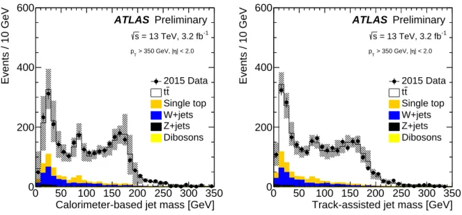
Figure 8 shows the distribution of the reconstructed jet mass in a sample of events enriched in top quark pair (t¯ t) events. The selection is based on the Run 1 in-situ JMS/JMR measurement [48] and is summar- ized here for completeness. Single-muon triggers are used to reject most of the events from QCD multijet background processes. t t ¯ events are chosen by requiring a muon with p

> 25 GeV and |η | < 2.5, as well as a missing transverse momentum E

> 20 GeV. The muons are required to satisfy a series of quality criteria, including isolation.8 The events are rejected if there is an additional muon. In addition, the sum of the E

and the transverse mass 9 of the W boson, reconstructed from the lepton and E

, is required to be greater than 60 GeV. Events must have at least one b-tagged jet (at the 70% efficiency working point for jets containing b-hadrons) and have at least one large-radius trimmed jet with p

> 200 GeV and

|η | < 2. Furthermore, there must be a small-radius jet with p

> 25 GeV, and ∆R < 1.5 to the selected lepton (targeting the decay chain t → bW ( → µν)). The resulting event purity is better than 70%. As expected, there are three mass peaks in Fig. 8 corresponding to the top quark mass, W boson mass, and the quark / gluon Sudakov peak. The W boson mass peak is more pronounced than the top quark mass peak due to the relatively low p

. For p

& 200 GeV, the track-assisted jet mass resolution is significantly larger than the calorimeter-based jet mass, which is why the W-boson mass peak is broader for the top right plot of Fig. 8. The top quark mass peak is enhanced at higher p

in Fig. 9.

8

Muon are considered isolated if they are well separated from jets (∆R > 0.4) and the track / calorimeter energy within a small cone, centered on the lepton direction but excluding the lepton itself, is below a fixed relative value.

9

The transverse mass, m

, is defined as m

= 2p

E

(1 − cos(∆φ)), where ∆φ is the azimuthal angle between the muon

and the direction of the missing transverse momentum.

Calorimeter-based jet mass [GeV]

0 50 100 150 200 250 300 350

Events / 10 GeV

0 500 1000 1500 2000 2500

2015 Data t

t

Single top W+jets Z+jets Dibosons ATLAS Preliminary

= 13 TeV, 3.2 fb

s

| < 2.0 η > 200 GeV, | pT

Track-assisted jet mass [GeV]

0 50 100 150 200 250 300 350

Events / 10 GeV

0 500 1000 1500 2000 2500

2015 Data t

t

Single top W+jets Z+jets Dibosons ATLAS Preliminary

= 13 TeV, 3.2 fb

s

| < 2.0 η > 200 GeV, | pT

Figure 8: The calorimeter-based jet mass distribution (left) and the track-assisted jet mass distribution (right) for jets with p

> 200 GeV. The MC is normalized to the data event yield. The uncertainty band includes systematic uncertainties related to the modeling of t ¯ t and the jet energy / mass scale uncertainties. See Sec. 9 for details.

Calorimeter-based jet mass [GeV]

0 50 100 150 200 250 300 350

Events / 10 GeV

0 200 400 600

2015 Data t

t

Single top W+jets Z+jets Dibosons ATLAS Preliminary

= 13 TeV, 3.2 fb

s

| < 2.0 η > 350 GeV, | pT

Track-assisted jet mass [GeV]

0 50 100 150 200 250 300 350

Events / 10 GeV

0 200 400 600

2015 Data t

t

Single top W+jets Z+jets Dibosons ATLAS Preliminary

= 13 TeV, 3.2 fb

s

| < 2.0 η > 350 GeV, | pT

Figure 9: The calorimeter-based jet mass distribution (left) and the track-assisted jet mass distribution (right) for

jets with p

> 350 GeV. The MC is normalized to the data event yield. The uncertainty band includes systematic

uncertainties related to the modeling of t¯ t and the jet energy / mass scale uncertainties. See Sec. 9 for details.

9 In-situ Mass and Energy Scale and Resolution

Top quark pair production provides an abundant source of hadronically decaying top quark and W boson jets that can be used to study the reconstruction of the jet four-vector in-situ. 10 One approach is the forward-folding method [48], in which particle-level spectra are folded by a modified detector response in order to best fit the reconstructed data. The resolution function that describes the transition from particle- level quantities x

to calibrated detector-level quantities x

is stretched and shifted so that the average value of x

in a fixed truth bin hx

| x

, p

i is scaled by s and the resolution is independently scaled by r:

x

| x

, p

= sx

+

x

− hx

| x

, p

i

(r − s), (7)

where x

| x

, p

is the folded quantity for a jet with x

and p

. By construction, x

= x

when s = r = 1 and x

= x

if s = 1, r = 0, and the method closes so that hx

| x

, p

i = x

. A two-dimensional χ

fit is performed to determine the values s

and r

such that the folded distribution best fits the data. By construction, fitting the simulation to itself results in s

= r

= 1.

To extract the jet mass scale and resolution, Eq. 7 is applied to the jet mass spectrum in one-lepton t¯ t events (see Sec. 8). The W-boson and top-quark resonance peaks are due to the combination of final-state radiation and the detector response. Taking the particle-level jet mass distribution as input, the relative jet mass scale and jet mass resolution can be extracted from forward-folding.

An improvement in the √

s = 13 TeV measurement with respect to the √

s = 8 TeV result in Ref. [48]

is the addition of jet energy scale and resolution constraints using the same forward-folding method.

Top-quarks in t¯ t events tend to be produced with similar transverse momenta and so the ratio of the hadronically decaying top quark to leptonically decaying top quark transverse momentum, p

/p

, is sensitive to the energy scale and resolution of the top quark jet. The leptonically decaying top quark is reconstructed from the selected lepton, the missing transverse momentum, and the close-by b-jet used in the event selection (see Sec. 8). The balance of the leading large-radius calorimeter jet p

with a partially reconstructed leptonically decaying top quark p

from only the lepton (p

) or the lepton and the close- by jet (p

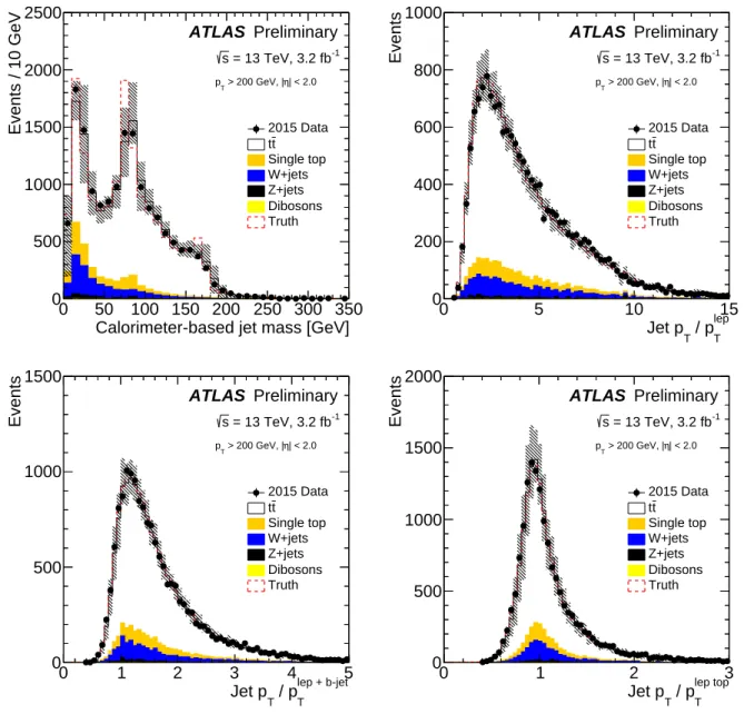
) is also considered due to their reduced systematic uncertainty from the calorimeter energy scale. Figure 10 shows the calorimeter-based jet mass as well as the three reconstructed top-quark transverse momentum ratio distributions. The p

ratio with the fully reconstructed leptonically decaying top quark has the sharpest peak because it contains the most information.

The χ

distributions marginalized over s or over r are shown in Fig. 11 and 12, respectively. The minima for the jet mass and energy resolutions are much flatter than for the corresponding scales because the resolutions in Fig. 10 are largely dominated by the physical resolution (from e.g. FSR). As expected from the relative size of the peaks in Fig. 10, the leptonically decaying top quark transverse momenta ratio is the most sensitive to the relative scale and resolution.

Table 2 summarizes the fitted values and systematic uncertainties. The jet mass scale and resolution of calorimeter-based jets are compared with the results obtained on √

s = 8 TeV data in Fig. 13. The mass scale and resolution of the track-assisted jet mass and reclustered jets are presented in Fig. 14.

10

The studies presented in this section are not currently used as the default uncertainties applied by analyses - see Sec. 7 for

the current jet mass scale uncertainties. These in-situ studies may be used in the future, but additional studies are required to

extend their validity beyond the presented kinematic regime.

Calorimeter-based jet mass [GeV]

0 50 100 150 200 250 300 350

Events / 10 GeV

0 500 1000 1500 2000 2500

2015 Data t t Single top W+jets Z+jets Dibosons Truth

ATLAS Preliminary

= 13 TeV, 3.2 fb

s

| < 2.0 η > 200 GeV, | pT

lep

/ p

Jet p

0 5 10 15

Events

0 200 400 600 800 1000

2015 Data t t Single top W+jets Z+jets Dibosons Truth

ATLAS Preliminary

= 13 TeV, 3.2 fb

s

| < 2.0 η > 200 GeV, | pT

lep + b-jet

/ p

Jet p

0 1 2 3 4 5

Events

0 500 1000 1500

2015 Data t t Single top W+jets Z+jets Dibosons Truth

ATLAS Preliminary

= 13 TeV, 3.2 fb

s

| < 2.0 η > 200 GeV, | pT

lep top

/ p

Jet p

0 1 2 3

Events

0 500 1000 1500 2000

2015 Data t t Single top W+jets Z+jets Dibosons Truth

ATLAS Preliminary

= 13 TeV, 3.2 fb

s

| < 2.0 η > 200 GeV, | pT

Figure 10: The distribution of the calorimeter-based jet mass (top left) and the jet p

divided by various reference transverse momenta: charged lepton p

(top right), combined with the nearest b-jet momentum (bottom left), further combined with the E

(bottom right). The truth histograms show the distribution of the particle-level jet mass (top left) or the particle-level jet p

divided by the detector-level reference momentum (top right and bottom).

The uncertainty band includes systematic uncertainties related to the modeling of t t ¯ and the jet energy / mass scale uncertainties. See the text for details.

The jet mass scale and the resolution extracted from the data have a sizeable statistical uncertainty and may be affected by a bias due to imperfections in the modelling of physics process or other aspects of the experimental response.

The most relevant experimental uncertainties are those which change the shape of the jet p

or jet mass

distributions. The jet energy scale and jet energy resolution systematics are the most relevant systematic

uncertainties for the jet mass. Pile-up doesn’t strongly a ff ect trimmed large-radius jets. Therefore, the

Relative jet mass scale

0.9 0.95 1 1.05 1.1

/NDF

χ

0 5 10 15 20 25

30 ATLAS Preliminary

= 13 TeV, 3.2 fb

s

| < 2.0 η > 200 GeV, | pT

Calorimeter-based jet mass

scale Relative jet p

0.9 0.95 1 1.05 1.1

/NDF

χ

0 2 4 6 8 10 12 14

16 ATLAS Preliminary

= 13 TeV, 3.2 fb

s

| < 2.0 η > 200 GeV, | pT

lep / pT Jet pT

scale Relative jet p

0.9 0.95 1 1.05 1.1

/NDF

χ

0 5 10 15 20

25 ATLAS Preliminary

= 13 TeV, 3.2 fb

s

| < 2.0 η > 200 GeV, | pT

lep + b-jet / pT Jet pT

scale Relative jet p

0.9 0.95 1 1.05 1.1

/NDF

χ

0 10 20 30 40 50 60

Preliminary ATLAS

= 13 TeV, 3.2 fb

s

| < 2.0 η > 200 GeV, | pT

lep top / pT Jet pT

Figure 11: The χ

per degrees of freedom, marginalized over the relative jet mass or jet transverse momentum scale for the calorimeter-based jet mass (top left), the jet p

using the ratio p

/p

(top right), the jet p

using the ratio p

/p

(bottom left), and the jet p

using the ratio p

/p

(bottom right).

associated systematic is small enough to be included as a component of JES uncertainty. Three different scenarios are used to study the correlation between small-R jets and large-R jet uncertainties and no large differences are seen. The b-tagging, E

and lepton systematic uncertainties are small, since they affect mostly the acceptance.

Uncertainties in the modelling of the t¯ t production process, top quark decay and fragmentation of the

hadronic final state are the largest source of systematic uncertainty. The shape of the particle-level dis-

tributions and the distribution of the energy inside a jet depend on the modelling of fragmentation, as

well as initial and final state radiation. To take into account these e ff ects, the fit is repeated with several

Relative jet mass resolution 0.4 0.6 0.8 1 1.2 1.4 1.6 1.8 /NDF

χ

0 5 10 15 20

25 ATLAS Preliminary

= 13 TeV, 3.2 fb

s

| < 2.0 η > 200 GeV, | pT

Calorimeter-based jet mass

resolution Relative jet p

0.4 0.6 0.8 1 1.2 1.4 1.6 1.8 /NDF

χ

0 5 10 15 20 25

30 ATLAS Preliminary

= 13 TeV, 3.2 fb

s

| < 2.0 η > 200 GeV, | pT

lep / pT Jet pT

resolution Relative jet p

0.4 0.6 0.8 1 1.2 1.4 1.6 1.8 /NDF

χ

0 10 20 30 40 50 60

70 ATLAS Preliminary

= 13 TeV, 3.2 fb

s

| < 2.0 η > 200 GeV, | pT

lep + b-jet / pT Jet pT

resolution Relative jet p

0.4 0.6 0.8 1 1.2 1.4 1.6 1.8 /NDF

χ

0 20 40 60 80 100

120 ATLAS Preliminary

= 13 TeV, 3.2 fb

s

| < 2.0 η > 200 GeV, | pT

lep top / pT Jet pT

Figure 12: The χ

per degrees of freedom, marginalized over the relative jet mass or jet transverse momentum resolution for the calorimeter-based jet mass (top left), the jet p

using the ratio p

/p

(top right), the jet p

using the ratio p

/p

(bottom left), and the jet p

using the ratio p

/p

(bottom right).

Monte Carlo generators. The uncertainty due to the NLO subtraction scheme is estimated by comparing

a Powheg + Herwig sample with a MC@NLO + Herwig sample. The e ff ect of using di ff erent fragmenta-

tion models is estimated by comparing Powheg+Pythia and Powheg+Herwig samples. Uncertainties due

to initial and final state radiation are estimated by comparing t¯ t Monte Carlo generators with different

factorisation / renormalisation scales, as well as the Perugia radLo / radHi tunes.

Quantity Value Stat. Uncert Modeling Jets Total Syst.

m

s

0.984 0.6 % 1.7 % 1.6 % 2.3 %

m

r

1.047 6.6 % 18.1 % 7.0 % 19.4 %

m

s

0.981 1.1 % 2.4 % 4.8 % 5.3 %

m

r

1.036 6.1 % 14.6 % 5.0 % 15.5 %

p

/p

s

1.011 0.7 % 1.3 % 0.4 % 1.3 %

p

/p

r

0.945 4.1 % 6.8 % 2.7 % 7.3 %

p

/p

s

0.985 0.4 % 0.7 % 1.2 % 1.4 % p

/p

r

0.903 6.1 % 5.5 % 4.7 % 7.2 % p

/p

s

0.987 0.2 % 0.3 % 2.1 % 2.1 % p

/p

r

1.024 3.1 % 6.2 % 6.0 % 8.6 %

Table 2: Summary of the systematic uncertainties for the relative jet mass or energy scales (s

) and resolutions (r

). The first column states which observable is used to extract the relative jet mass (first four rows) or jet energy (rows 5-10) scale and resolutions.

Relative Jet Mass Scale

0.8 0.9 1 1.1 1.2

Relative Jet Mass Resolution

0.6 0.8 1 1.2

1.4 ATLAS Preliminary

| < 2.0 η > 200 GeV, | pT

stat. uncertainty σ

Data 1

syst. uncertainty

⊕ Data stat

8 TeV, 20.3 fb-1

13 TeV, 3.2 fb-1

Figure 13: The relative jet mass scale and relative jet mass resolution extracted from the √

s = 8 TeV dataset for large-radius trimmed calorimeter jets with a subjet size of R

= 0.3 [48] and the values extracted from the √

s = 13

TeV dataset with R

= 0.2.

Relative Jet Mass Scale

0.8 0.9 1 1.1 1.2

Relative Jet Mass Resolution

0.5 1 1.5

ATLAS Preliminary

= 13 TeV, 3.2 fb

s

| < 2.0 η > 200 GeV, | pT

mcalo

mTA

stat. uncertainty σ

Data 1

syst. uncertainty

⊕ Data stat

Figure 14: The relative jet mass scale and relative jet mass resolution for calorimeter-based jet mass (blue) and

track-assisted jet mass (red)

10 Improving the Track-assisted Jet Mass

As discussed in Section 6, the performance of track-assisted jet mass depends on the p

regime and the topology of the signal jet. In this section, several explored techniques which have the potential to improve the performance of the track-assisted jet mass are discussed.

10.1 Combination with the calorimeter-based jet mass

As the calorimeter-based jet mass is not used explicitly in the construction of the track-assisted jet mass, it may be possible to reduce the response resolution by combining information from both mass definitions.

Fluctuations in the calorimeter energy response impact both the calorimeter-based jet mass and p

re- sponse. However, the p

response is not as sensitive to the local distribution of fluctuations and therefore the jet p

response and the calorimeter-based jet mass response are nearly independent. The correlation is slightly higher at lower p

, where the the decay products are more spread out and thus the p

and mass are more related. Figure 15 shows the track-assisted jet mass response vs the calorimeter-based jet mass response for jets with p

> 1 TeV where the correlation coe ffi cient is ∼ 10%. Due to the approximate independence and Gaussian nature of the p

and mass responses, the optimal combination of the two variables is linear: 11 m

= a × m

+ b × m

. For calibrated m

and m

, the combined jet mass is also calibrated if a + b = 1. Using this constraint and minimizing the resolution of the m

response results in the nearly optimal weights:

a = σ

σ

+ σ

b = σ

σ

+ σ

, (8)

where σ

and σ

are the calorimeter-based jet mass resolution function and the track-assisted mass resolution function respectively. Figure 16 shows the resolution of the calorimeter-based jet mass and the track-assisted jet mass (as in Fig. 6), but additionally shows the resolution of the combined jet mass for W-jets. The combined jet mass smoothly interpolate between m

∼ m

at low p

and m

∼ m

at high p

. As expected, the combined jet mass resolution is never larger than either of the input jet masses. For top-jets, since the calorimeter-based jet mass performs best in all p

range, the combined jet mass will be mostly weighted by the calorimeter-based jet mass contribution and the resolution of the combined jet mass is as good as the calorimeter-based jet mass.

Systematic uncertainties on the combined jet mass are estimated by propagating uncertainties on m

and m

through the linear combination defining m

. Just as the tracking r

uncertainties for the calorimeter jet p

are treated as fully correlated with the tracking uncertainties on m

and p

, the tracking r

uncertainties for the calorimeter-based jet mass are also fully correlated with all of the tracking uncertainties.

11

If the joint distribution of the responses is Gaussian, then one can write their probability distribution function as f ( x, y) =

h( x, y) × exp[A( µ) + T (x, y) µ], where x is the calorimeter-based jet mass response, y is the track-assisted jet mass response,

µ is the common average response, and h, A,T are real-valued functions. This form shows that the distribution is from the

exponential family and therefore T is a sufficient statistic. Since the natural parameter space is one-dimensional, T is also

complete. Therefore, the unique minimal variance unbiased estimator of µ is the unique unbiased function of T (x, y) =

x/σ

+ y/σ

. See e.g. Ref. [49] for details.

Arbitrary units

0 10 20

truth TA

/ m m

0.5 1 1.5

truth

/ m

m

0.5 1 1.5

Simulation Preliminary ATLAS

| < 2

> 250 GeV, | = 13 TeV, W/Z-jets, p

s

correlation = 0.22

Arbitrary units

0 2 4 6

truth TA

/ m m

0.5 1 1.5

truth

/ m

m

0.5 1 1.5

Simulation Preliminary ATLAS

| < 2

> 1 TeV, | = 13 TeV, W/Z-jets, p

s

correlation = 0.10

Figure 15: The calorimeter-based jet mass response vs the track-assisted jet mass response for W / Z-jets produced from with p

> 250 GeV (left) and p

> 1 TeV (right).

[GeV]

Truth jet p T

500 1000 1500 2000 2500

) m ) / median(R m 68% IQnR(R × 2 1

0.05 0.1 0.15

0.2 0.25 0.3

Simulation Preliminary ATLAS

| < 0.8 η = 13 TeV, W/Z-jets, | s

truth reco

/m

m

= m R

m

m

m

Figure 16: The jet mass resolution vs jet p

for calorimeter-based jet mass (blue solid line), track-assisted jet mass (red dashed line), and the combined jet mass (black dotted line) for W / Z-jets. Note that since the response distri- butions are non-Gaussian, the linear combination of the two mass definitions is slightly non-optimal in the lowest bins; the combined resolution (in terms of the IQnR) is not exactly σ

combined

= aσ

calo

+ bσ

TA

.