ATLAS-CONF-2016-024 02June2016
ATLAS NOTE
ATLAS-CONF-2016-024
1st June 2016
Electron efficiency measurements with the ATLAS detector using the 2015 LHC proton-proton collision data
The ATLAS Collaboration
Abstract
This note summarises the electron efficiency measurements using the 2015 LHCppcollision data at 13 TeV centre-of-mass energy. The data, collected by the ATLAS detector, correspond to an integrated luminosity of 3.2 fb−1. The studies are focused on electron reconstruction, identification, trigger and isolation algorithms. The combination of these algorithms leads to a large variety of operating points for the electron measurement, with diverse signal efficiency versus background rejection performance. Samples of electron candidates with transverse energies above 7 GeV, in the central region of the detector defined by the pseudorapidity range |η| < 2.47 are selected using the tag-and-probe method for Z → ee and J/ψ → ee processes. The measurements performed on data are compared to the measurements done on Monte Carlo simulations in the same phase space. The deviations are expressed as data- to-MC ratios, which are provided for a variety of operating points, and used in the physics analyses in order to correct the Monte Carlo simulations.
© 2016 CERN for the benefit of the ATLAS Collaboration.
Reproduction of this article or parts of it is allowed as specified in the CC-BY-4.0 license.
1. Introduction
In the ATLAS detector [1], electrons and positrons, collectively referred to as electrons, in the central region1give rise to tracks in the inner detector and energy deposits in the electromagnetic calorimeter.
The calorimeter signals are used in the first level trigger system (L1), and are combined with tracks to reconstruct electron candidates used for the high level trigger (HLT) decision algorithms.
The electron candidates are then further selected against background – such as hadrons and background (non-prompt) electrons originating predominantly from photon conversions and heavy flavour hadron decays – using several sets of identification criteria with different levels of background rejection and signal efficiency. These identification criteria rely on the shapes of electromagnetic showers in the calorimeter as well as on tracking and track-to-cluster matching quantities. Additionally, electrons can be required to be isolated from other activity in the calorimeter or inner detector to further distinguish them from background objects.
The accuracy of the Monte Carlo (MC) detector simulation to model the electron measurement efficiency plays a crucial role for cross section measurements and searches for new physics. In order to achieve reliable results, the MC samples are corrected to reproduce the efficiencies measured with data. The efficiency measurements of the various steps described above (trigger, reconstruction, identification and isolation) are based on the tag-and-probe method using the Z and the J/ψ resonances, requiring the presence of an isolated identified electron as the tag. The data measurements are compared to the simulation to obtain corrections (scale-factors) as a function of the electron’s transverse energyETand its pseudorapidityη. Previous efficiency measurements were performed for Run-1 data at 7 TeV [2] and 8 TeV [3] centre-of-mass energy.
This note contains the description of the electron reconstruction, identification, isolation and trigger algorithms, as well as the measurements of the corresponding experimental efficiencies for the data collected at a centre-of-mass energy of 13 TeV in 2015 and with 25ns bunch spacing. During this period, the ATLAS detector recorded a data sample corresponding to an integrated luminosity of 3.2 fb−1with all relevant detector components fully functional. The methodology used to extract the various efficiency measurements follows, with small modifications, the one used during Run-1 and described in Ref. [3].
A brief description of the ATLAS detector is presented in Sect.2. The description of various algorithms together with the optimisations performed in order to adapt these algorithms to the Run-2 running conditions are described in Sects.3–6. The general methodology of the efficiency measurements and the data and Monte Carlo samples used in this work are presented in Sect. 7. Sect. 8 describes the identification efficiency measurement, while Sect.9, Sect. 10 and Sect. 11 present the reconstruction, isolation and trigger efficiency measurements, respectively. Sect.12contains the conclusions.
1ATLAS uses a right-handed coordinate system with its origin at the nominalppinteraction point at the centre of the detector.
The positivex-axis is defined by the direction from the interaction point to the centre of the LHC ring, with the positivey-axis pointing upwards, while the nominal beam direction defines thez-axis. The transverse momentapT and transverse energies ET (used thereafter for calorimetric measurements) are measured in the x−yplane. The azimuthal angleφis measured around the beam axis and the polar angleθis the angle from thez-axis. The pseudorapidity is defined asη=−ln tan(θ/2). The radial distance between two objects is defined as∆R=q
∆η2+∆φ2. This note describes measurements performed in the central region, defined by|η|<2.47.
2. The ATLAS Detector
A complete description of the ATLAS detector is provided in Ref. [1].
The inner detector provides a precise reconstruction of tracks within|η| < 2.5. It consists of four layers of pixel detectors close to the beam-pipe, four layers of silicon microstrip detector modules (SCT) with pairs of single-sided sensors glued back-to-back, and a transition radiation tracker (TRT) at the outer radii (in the range |η| < 2.0). A track from a charged particle traversing the barrel detector typically has 12 silicon measurement points (hits), of which four are pixel and eight SCT hits, and approximately 35 TRT straw hits.
The innermost pixel layer, the insertable B-layer (IBL) [4], was added between Run-1 and Run-2 of the LHC. It is composed of 14 lightweight staves arranged in a cylindrical geometry, each made of 12 silicon planar sensors in its central region and four 3D sensors at each end. The IBL pixel dimensions are 50×250µm2in theφandzdirections (compared with 50×400µm2for other pixel layers). The smaller radius and the reduced pixel size result in improvements of both the transverse and longitudinal impact parameter resolutions. Moreover, new detector services for the pixel detector have been implemented which significantly reduce the material at the boundaries of the active tracking volume.
The TRT offers substantial discrimination between electrons and charged hadrons over a wide energy range through the detection of transition radiation photons. During Run-1, several leaks developed in the TRT exhaust system, leading to a large loss of highly expensive xenon gas. In order to reduce the operation costs in 2015, a few parts of the TRT (internal layer of the Barrel TRT and one endcap wheel on each side of the detector) were running with argon gas mixture.
The central electromagnetic (EM) calorimeter is a lead-liquid argon sampling calorimeter with accordion- shaped electrodes and lead absorber plates. It is divided into a barrel section (EMB) covering|η| <1.475 and two endcap sections (EMEC) covering 1.375 < |η| < 3.2. For |η| < 2.5, it is divided into three longitudinal layers and offers a fine segmentation in the lateral direction of the showers. At high energy, most of the EM shower energy is collected in the middle layer, which has a lateral granularity of 0.025× 0.025 inη×φspace. The first (strip) layer consists of finer-grained strips segmented in theη-direction with a coarser granularity inφ. It provides excellentγ−π0discrimination and a precise estimation of the pseudorapidity of the impact point. The back layer collects the energy deposited in the tail of high energy EM showers. A thin pre-sampler detector, covering|η| <1.8, is used to correct for fluctuations in upstream energy losses. The transition region between the EMB and EMEC calorimeters, 1.37< |η| <1.52, has a large amount of material in front of the first active calorimeter layer.
Hadronic calorimeters with at least three longitudinal segments surround the EM calorimeter and are used in this context to reject hadronic jets. The forward calorimeters cover the range 3.1 < |η| < 4.9 and also have EM shower identification capabilities given their fine lateral granularity and longitudinal segmentation into three layers.
3. Electron Reconstruction
Electron reconstruction in the central region of the ATLAS detector (|η| < 2.47) proceeds in several steps:
• Seed-cluster reconstruction: A sliding window with a size of 3×5 in units of 0.025×0.025, corresponding to the granularity of the EM calorimeter middle layer, inη×φspace is used to search for electron cluster "seeds" as longitudinal towers2 with total cluster transverse energy above 2.5 GeV. The clusters are then formed around the seeds using a clustering algorithm [5] that allows for duplicates to be removed. The cluster kinematics are reconstructed using an extended window depending on the cluster position in the calorimeter. The efficiency of this cluster search ranges from 95% atET =7 GeV to more than 99% aboveET=15 GeV.
• Track reconstruction: Track reconstruction proceeds in two steps: pattern recognition and track fit. The standard ATLAS pattern recognition uses the pion hypothesis for energy loss due to interactions with the detector material. This has been complemented with a modified pattern recognition algorithm which allows up to 30% energy loss at each intersection of the track with the detector material to account for possible bremsstrahlung. If a track seed (consisting of three hits in different layers of the silicon detectors) with a transverse momentum larger than 1 GeV can not be successfully extended to a full track of at least seven hits using the pion hypothesis and it falls within one of the EM cluster region of interest3, a second attempt is performed with the new pattern recognition using an electron hypothesis that allows for larger energy loss. Track candidates are then fit either with the pion hypothesis or the electron hypothesis (according to the hypothesis used in the pattern recognition), using the ATLAS Global χ2Track Fitter [6]. If a track candidate fails the pion hypothesis track fit (for example, due to large energy losses), it is refit with the electron hypothesis. In this way, a specific electron-oriented algorithm has been integrated into the standard track reconstruction. It improves the performance for electrons and has minimal interference with the main track reconstruction.
• Electron specific track fit: The obtained tracks are loosely matched to EM clusters using the distance in η and φ between the position of the track, after extrapolation, in the calorimeter middle layer and the cluster barycentre. The matching conditions account for energy-loss due to bremsstrahlung and the number of precision hits in the silicon detector. Tracks that have significant number of precision hits (≥ 4) and are loosely associated to electron clusters are refit using an optimised Gaussian Sum Filter (GSF) [7], which takes into account the non-linear bremsstrahlung effects.
• Electron candidate reconstruction: The matching of the track candidate to the cluster seed completes the electron reconstruction procedure. A similar matching as the one described above is repeated for the refit track with stricter conditions.
If several tracks fullfil the matching condition, one track is chosen as "primary" track. The choice is based on an algorithm using the cluster-track distance Rcalculated using different momentum hypotheses, the number of pixel hits and the presence of a hit in the first silicon layer [3]. Electron candidates without any associated precision hit tracks are removed and considered to be photons.
The efficiency of this association and subsequent track quality cuts is measured as the "reconstruction efficiency" in Sect.9. The electron cluster is then re-formed using 3×7 (5×5) longitudinal towers
2Theη×φspace of the EM calorimeter is divided into a grid ofNη×Nφ=200×256 elements of size∆ηtower×∆φtower= 0.025×0.025, called towers. Inside each of these elements, the energy of cells in all longitudinal layers (including the front, middle, and back calorimeter layers as well as, for |eta| < 1.8, the presampler) is summed into the tower energy, with the energy of cells spanning several towers distributed uniformly among the participating towers.
3For each seed EM cluster passing loose shower shape requirements ofRη >0.65 andRhad<0.1 (for the definition of these variables, see Table1) a region of interest with a cone-size of∆R=0.3 around the seed cluster barycenter is defined.
of cells in the barrel (endcaps) of the EM calorimeter. The energy of the clusters is calibrated to the original electron energy using multivariate techniques [8] based on simulated MC samples.
The four-momentum of the electrons is computed using information from both the final calibrated energy cluster and the best track matched to the original seed cluster. The energy is given by the final calibrated cluster, while theφandηdirections are taken from the corresponding track parameters with respect to the beam-line.
For Run-2 analyses, the electron measurements are performed by requiring the track associated with the electron to be compatible with the primary interaction vertex of the hard collision, in order to reduce the background from conversions and secondary particles. The track parameters are calculated in a reference frame where the z-axis is taken along the measured beam-line position. The following conditions are applied together with all the identification operating points considered in this note: d0/σd0 < 5 and
∆z0sinθ <0.5 mm, where the impact parameterd0is the distance of closest approach of the track to the measured beam-line,z0 is the distance along the beam-line between the point whered0is measured and the beam-spot position, andθis the polar angle of the track. To assess the compatibility with the primary vertex of the hard collision the∆z0 between the track and the primary vertex is employed. This vertex is selected from the reconstructed primary vertices (compatible with the beam-line) as the one with the highest sum of transverse momenta of the associated tracks. σd0represents the estimated uncertainty of thed0 parameter, andθ is the polar angle of the track. The efficiency of these requirements in data and MC is estimated together with the efficiency of the various identification operating points.
4. Electron Identification
To determine whether the reconstructed electron candidates are signal-like objects or background-like objects such as hadronic jets or converted photons, algorithms for electron identification (ID) are applied.
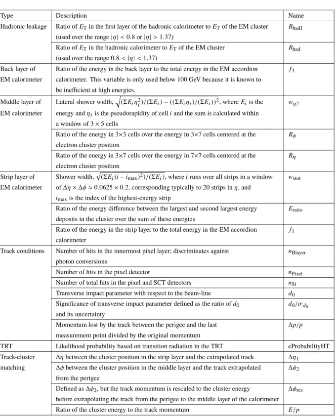
The ID algorithms use quantities related to the electron cluster and track measurements including calor- imeter shower shapes, information from the transition radiation tracker, track-cluster matching related quantities, track properties, and variables measuring bremsstrahlung effects for distinguishing signal from background. These quantities are summarised in Table1.
For Run-2, several changes to the input variables used for electron ID have been introduced. Taking advantage of the IBL, the number of hits in this innermost pixel layer is used for discriminating between electrons and converted photons. This criterion was also used in Run-1, but with what is now the second-to-innermost pixel layer.
Moreover, the change in the TRT gas led to modifications in the detector response and prompted the introduction of a new discriminating variable in the electron identification algorithms. In Run-1, only the fraction of high-threshold hits was used from the TRT as a signature of transition radiation to distinguish electrons from hadrons. In Run-2, a likelihood method based on the TRT high-threshold hits is introduced to compensate for the lower transition radiation absorption probability of the argon. The TRT likelihood method uses the high-threshold probability of each TRT hit to construct a discriminant variable, referred to here as eProbabilityHT. The probability for each TRT hit to exceed the high level threshold depends on the straw gas type, the Lorentz factorγcalculated from the track pT under a particle type hypothesis, and the geometry: detector partition, straw layer, track-to-wire distance and the hit coordinates (z for the barrel and radius for the endcaps).
Table 1: Definitions of electron discriminating variables.
Type Description Name
Hadronic leakage Ratio ofETin the first layer of the hadronic calorimeter toETof the EM cluster Rhad1 (used over the range|η|<0.8 or|η|>1.37)
Ratio ofETin the hadronic calorimeter toETof the EM cluster Rhad (used over the range 0.8<|η|<1.37)
Back layer of Ratio of the energy in the back layer to the total energy in the EM accordion f3 EM calorimeter calorimeter. This variable is only used below 100 GeV because it is known to
be inefficient at high energies.
Middle layer of Lateral shower width, q
(ΣEiη2i)/(ΣEi)−((ΣEiηi)/(ΣEi))2, whereEiis the wη2 EM calorimeter energy andηiis the pseudorapidity of celliand the sum is calculated within
a window of 3×5 cells
Ratio of the energy in 3×3 cells over the energy in 3×7 cells centered at the Rφ electron cluster position
Ratio of the energy in 3×7 cells over the energy in 7×7 cells centered at the Rη
electron cluster position Strip layer of Shower width,
p(ΣEi(i−imax)2)/(ΣEi), whereiruns over all strips in a window wstot EM calorimeter of∆η×∆φ≈0.0625×0.2, corresponding typically to 20 strips inη, and
imaxis the index of the highest-energy strip
Ratio of the energy difference between the largest and second largest energy Eratio deposits in the cluster over the sum of these energies
Ratio of the energy in the strip layer to the total energy in the EM accordion f1 calorimeter
Track conditions Number of hits in the innermost pixel layer; discriminates against nBlayer photon conversions
Number of hits in the pixel detector nPixel
Number of total hits in the pixel and SCT detectors nSi
Transverse impact parameter with respect to the beam-line d0 Significance of transverse impact parameter defined as the ratio ofd0 d0/σd
0
and its uncertainty
Momentum lost by the track between the perigee and the last ∆p/p measurement point divided by the original momentum
TRT Likelihood probability based on transition radiation in the TRT eProbabilityHT Track-cluster ∆ηbetween the cluster position in the strip layer and the extrapolated track ∆η1
matching ∆φbetween the cluster position in the middle layer and the track extrapolated ∆φ2 from the perigee
Defined as∆φ2, but the track momentum is rescaled to the cluster energy ∆φres before extrapolating the track from the perigee to the middle layer of the calorimeter
Ratio of the cluster energy to the track momentum E/p
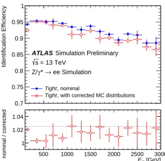
The re-optimisation of the ID algorithms for Run-2 is based on MC simulation samples. Electron candidates from MC simulations of Z → ee and dijet events are used, in addition to J/ψ → ee and minimum bias events at lowET. However, the distributions of several input variables in data tend to be wider or shifted more towards the background distributions than in the MC, due to inaccuracies in the detector description and the modelling of the shower shapes in Geant [9]. To account for this, corrections derived from data in the form of simple linear shifts or width adjustments to the MC distributions were applied to the electron candidates’ distributions used in the optimisation, to ensure that the performance of the operating points derived in MC would correspond to the one observed in the data. This procedure is only used for the described optimisation, while MC samples used for physics analyses are corrected using event weights to account for mismodelling of tracking properties or shower shapes, and to reproduce the efficiencies measured with data.
The baseline ID algorithm used for Run-2 data analyses is the likelihood-based (LH) method. It is a multivariate analysis (MVA) technique that simultaneously evaluates several properties of the electron candidates when making a selection decision. The LH method uses the signal and background probability density functions (PDFs) of the discriminating variables4. Based on these PDFs, an overall probability is calculated for the object to be signal or background. The signal and background probabilities for a given electron are then combined into a discriminantdLon which a requirement is applied:
dL = LS
LS+LB, LS(B)(~x) =
n
Y
i=1
Ps(b),i(xi) (1)
where~xis the vector of discriminating variable values and Ps,i(xi) is the value of the signal probability density function of theith variable evaluated at xi. In the same way, Pb,i(xi) refers to the background probability function. This allows for better background rejection for a given signal efficiency than a
"cut-based" algorithm that would use selection criteria sequentially on each variable. In addition to the variables used as input to the LH discriminant, simple selection criteria are used for the variables counting the number of hits on the track.
Three levels of identification operating points are typically provided for electron ID. These are referred to, in order of increasing background rejection, asLoose,Medium, andTight. If not otherwise specified, the operating points will refer to the LH identification algorithm. TheLoose,MediumandTightoperating points are defined such that the samples selected by them are subsets of one another. Each operating point uses the same variables to define the LH discriminant, but the selection on this discriminant is different for each operating point. Thus, electrons selected byMediumare all selected byLoose, andTightelectrons are all selected byMedium.
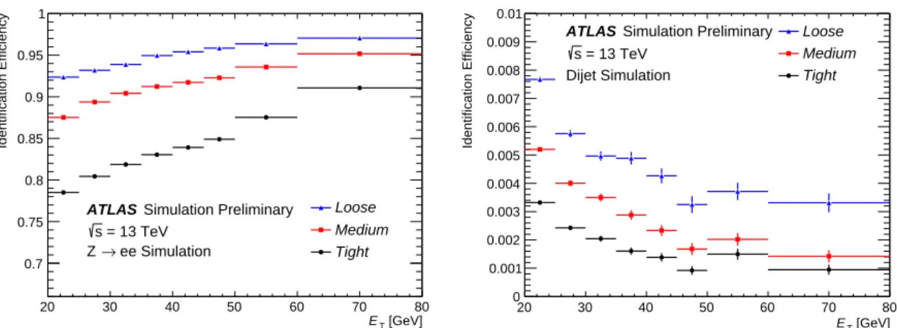
The distributions of electron shower shapes depend on the amount of material the electrons pass through, and therefore vary with the pseudorapidity of the electron candidates. In addition, significant changes to the shower shapes and track properties are expected with increasing energy. The ID operating points were consequently optimised in several bins in|η|andET. The performance of the LH identification algorithm is illustrated in Fig.1. Depending on the operating point, the signal (background) efficiencies for electron candidates withET= 25 GeV are in the range from 78 to 90% (0.3 to 0.8%) and increase (decrease) with ET.
4All variables presented in Table1are used as PDFs exceptE/p,wstotand∆φ2, and the variables counting the number of hits on the track. Simple selection criteria are always applied to the latter, while the first three are only used as rectangular cuts in either theTightoperating point at highETor the cut-based ID, as described below.
[GeV]
ET
20 30 40 50 60 70 80
Identification Efficiency
0.7 0.75 0.8 0.85 0.9 0.95 1
Simulation Preliminary ATLAS
= 13 TeV s
ee Simulation
→ Z
Loose Medium Tight
[GeV]
ET
20 30 40 50 60 70 80
Identification Efficiency
0 0.001 0.002 0.003 0.004 0.005 0.006 0.007 0.008 0.009 0.01
Simulation Preliminary ATLAS
= 13 TeV s
Dijet Simulation
Loose Medium Tight
Figure 1: The efficiency to identify electrons fromZ → eedecays (left) and the efficiency to identify hadrons as electrons (background rejection, right) estimated using simulated dijet samples. The efficiencies are obtained using Monte Carlo simulations, and are measured with respect to reconstructed electrons. The candidates are matched to true electron candidates forZ →eeevents. For background rejection studies the electrons matched to true electron candidates are not included in the analysis. Note that the last bin used for the optimisation of the ID is 45-50 GeV, which is why the signal efficiency increases slightly more in the 50 GeV bin than in others, and the background efficiency increases in this bin as well.
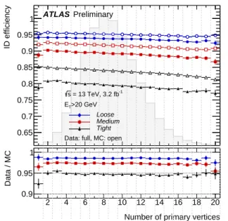
The electron identification performance may be influenced by the parasitic collisions taking place in the same beam crossing (in-time pileup) or a consecutive bunch crossing (out-of-time pileup) as the hardpp collision producing the electron candidate. The number of reconstructed primary vertices is indicative of the level of pileup in each event, with the average number of primary vertices (eight per event) corresponding to an average pileup of 13.7. Since some shower shape distributions depend on the number of pileup collisions per bunch crossing, the cut on the LH discriminant value is loosened as a function of the number of primary vertices. This is done to ensure that the LH identification remains efficient at high pileup, without drastically increasing the amount of background accepted by the LH selection. The optimisation included simulations with a number of pileup collisions of up to 40, covering the range of the pileup observed in 2015.
At high ET, some of the calorimeter variable distributions are different from the typical distributions obtained with Z → ee and used to construct the LH PDFs. Higher energy electrons tend to deposit relatively smaller fractions of their energy in the early layers of the EM calorimeter, and more in the later layers of the EM calorimeter or even in the hadronic calorimeter. LooseandMediumwere deemed to be loose enough to be robust against theseET-dependent changes. However, the tighter requirement used in Tightwould lead to inefficiencies at highET, if not handled properly. Thus, for electron candidates with ET above 125 GeV, Tightuses the same discriminant selection asMediumbut adds rectangular cuts on wstotandE/p, which were found to be particularly effective at discriminating signal from background at highET.
In addition to the multivariate approach used in the LH method described so far, a cut-based method using a set of rectangular cuts on the electron ID discriminating variables was used in Run-1. This method encompasses a similar set of operating points. The cut-basedLooseoperating point relies primarily on information from the hadronic calorimeter and the first two layers of the EM calorimeter for distinguishing signal from background. The cut-basedMedium operating point adds information from the TRT, the transverse impact parameter, and the third layer of the EM calorimeter, in addition to tighter cuts on the
variables from the cut-basedLoose ID. Finally, the cut-based Tight operating point adds track-cluster matching variables such as E/p and∆φ2, and uses tighter cuts than the cut-based MediumID for the remaining variables. The cut-based algorithms were optimised for Run-2 and used as for cross-checks during the 2015 data taking. These selection criteria are used in the analyses presented in this note for the background selections used in the tag-and-probe measurements. The cut-based algorithms are not used in physics analyses in Run-2 and therefore their efficiencies are not presented in this note.
5. Electron Isolation
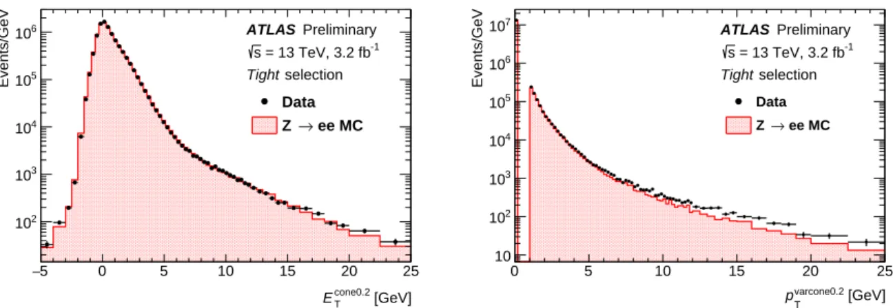
In addition to the identification criteria described above, most analyses require electrons to fulfil isolation requirements, to further discriminate between signal and background. The isolation variables quantify the energy of the particles produced around the electron candidate and allow to disentangle prompt electrons (from heavy resonance decays, such asW → eν, Z → ee) from other, non-isolated electron candidates such as electrons originating from converted photons produced in hadron decays, electrons from heavy flavour hadron decays, and light hadrons mis-identified as electrons. Two discriminating variables have been designed for that purpose:
• acalorimetricisolation energy, Econe0.2
T , defined as the sum of transverse energies of topological clusters [5, 10], calibrated at the electromagnetic scale, within a cone of ∆R = 0.2 around the candidate electron cluster. Only clusters with reconstructed positive energy are considered in the sum. TheET contained in a rectangular cluster of size∆η ×∆φ = 0.125×0.175 centred around the electron cluster barycentre is subtracted. An (ET, η) dependent correction is then applied to account for the electron energy leakage outside this cluster. The contribution from pileup and the underlying event activity is corrected for on an event-by-event basis using the technique outlined in Ref. [11]5;
• atrackisolation,pvarcone0.2
T , defined as the sum of transverse momenta of all tracks, satisfying quality requirements, within a cone of∆R=min(0.2,10 GeV/ET)around the candidate electron track and originating from the reconstructed primary vertex of the hard collision, excluding the electron associated tracks, i.e. the electron track and additional tracks from converted bremsstrahlung photons. The track quality requirements are :
– ET >1 GeV;
– nSi ≥ 7,nhole
Si ≤ 2,nhole
Pixel ≤ 1,nshmod ≤ 1, wherenhole
Si andnhole
Pixel are the number of missing hits in the silicon (pixel and SCT) and pixel detector respectively, andnsh
modis the number of hits in the silicon detector assigned to more than one track;
– |∆z0sinθ| <3 mm.
The distributions of these two discriminating variables are illustrated in Fig.2for electrons ofETgreater than 27 GeV satisfying theTight requirements, selected in events consistent with originating from the Z →eeprocess. The negative tail ofEcone0.2
T originates from the correction for pileup and the underlying event activity. A slight discrepancy is observed in the region at largeEcone0.2
T andpvarcone0.2
T values, where the background dominates (note that no background subtraction is applied here).
5To account for the variation of the ambient energy density as a function of the pseudorapidity, it is estimated in two wide pseudorapidity bins :|η|<1.5 and 1.5<|η|<3.0.
[GeV]
cone0.2
ET
−5 0 5 10 15 20 25
Events/GeV
102
103
104
105
106
Data ee MC
→ Z
ATLAS Preliminary = 13 TeV, 3.2 fb-1
s
selection Tight
[GeV]
varcone0.2
pT
0 5 10 15 20 25
Events/GeV
10 102
103
104
105
106
107
Data ee MC
→ Z
ATLAS Preliminary = 13 TeV, 3.2 fb-1
s
selection Tight
Figure 2: Distributions ofEcone0.2
T (left) andpvarcone0.2
T (right) for electrons fromZ →ee, in the data (dots with error bars) and the simulation (full histogram, normalised to data).
A variety of selection requirements on the quantitiesEcone0.2
T /ETandpvarcone0.2
T /EThave been defined to select isolated electron candidates. The resulting operating points are divided into two classes:
• efficiency targeted operating points: varying requirements are used in order to obtain a given isolation efficiencyεiso, which can be either constant or as a function of ET. Typical εiso values are 90(99)% for ET = 25(60) GeV, estimated for electrons from simulated Z → eeevents. For transverse energies between 7 and 15 GeV, simulated electrons fromJ/ψdecays have been used to determine the upper cuts onEcone0.2
T andpvarcone0.2
T , and only events satisfying∆φ > 0.3 have been considered, where∆φis the azimuthal separation between the two electrons.
• fixed requirement operating points: in this case the upper thresholds on the isolation variables are constant. These operating points were optimised by maximising the expected sensitivities of H →4`and multilepton supersymmetry searches.
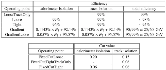
Table2shows the definition of the various operating points used for electron isolation. Fixed requirement operating points are typically preferred in physics analyses using low ET electrons and requiring high background rejection, while in the highETrange looser operating points are adopted in order to maintain high signal efficiency.
6. Electron Trigger
The ATLAS online data processing reconstructs and identifies electron candidates both at the L1 trigger and at the HLT. At L1, the electron triggers use the signals recorded in the electromagnetic (EM) and hadronic calorimeters within regions of 4×4 trigger "towers" (corresponding to∆η×∆φ≈0.4×0.4) to calculate the energy in the inner region (core) and the surrounding (isolation) region. TheETthresholds used in the trigger decision can be set differently for differentηregions that are delimited by theηvalues ofN ×0.1 (N = 1,2, ..). This allows a coarse tuning of thresholds taking into account different energy responses in different regions. A veto on the hadronic leakage can also be applied at L1 by requiring that the amount of energy measured in the hadronic calorimeter behind the core of the EM cluster relative to the EM cluster energy is less than a certain value. An isolation cut on the transverse energy in an annulus
Efficiency
Operating point calorimeter isolation track isolation total efficiency
LooseTrackOnly - 99% 99%
Loose 99% 99% ∼98%
Tight 96% 99% ∼95%
Gradient 0.1143%×ET+92.14% 0.1143%×ET+92.14% 90/99% at 25/60 GeV GradientLoose 0.057%×ET+95.57% 0.057%×ET+95.57% 95/99% at 25/60 GeV
Cut value
Operating point calorimeter isolation track isolation
FixedCutLoose 0.20 0.15
FixedCutTightTrackOnly - 0.06
FixedCutTight 0.06 0.06
Table 2: Electron isolation operating point definitions. The upper table illustrates the efficiency targeted operating points, and the numbers expressed in percents represent the target efficiencies used in the operating point optimisation procedure. For the Gradient and GradientLoose operating points,ETis in GeV. The fixed requirement operating points are shown in the lower table. The calorimeter and track isolation refer to the selection based onEcone0.2
T /ET andpvarcone0.2
T /ET, respectively.
of calorimeter towers around the EM candidate relative to the EM cluster transverse energy can also be used at L1. The isolation and hadronic leakage veto requirements are not used for electron candidates with a transverse energy of greater than 50 GeV.
At the HLT, electron candidates are reconstructed and selected in several steps to reject potential back- ground candidates early, thereby reducing the event rate to a level where more precise offline-like al- gorithms, using information from calorimeter and tracking, can be applied in the allowed latency range.
Fast EM calorimeter algorithms build clusters from the calorimeter cells within the region of interest (RoI) (∆η×∆φ = 0.4×0.4) identified at the L1 step, using the second layer of the EM calorimeter to find the cell with the largest deposited transverse energy in the RoI. Electrons are identified by applying requirements on the energy deposit in the hadronic calorimeter Rhad, on the Rη shower shape variable, onEratioas well as on the transverse energy of the cluster. Tracks reconstructed using a simplified (fast) tracking algorithm, with a minimumpTof 1 GeV, are associated to clusters within∆η <0.2. The second step of the HLT relies on precise offline-like algorithms, based on candidates selected in the first step. EM calorimeter clusters are built following the same techniques described in Sect.3. Additional requirements on the shower shapes are applied to reduce the rate further before precision tracking. Electrons are recon- structed with clusters matched to precision tracks extrapolated to the second layer of the EM calorimeter within|∆η| < 0.05 and|∆φ| < 0.05. The ID of electrons at the HLT is performed employing the same discriminating variables as the offline ID described in Sect.4.
During Run-1, the electron trigger used a cut-based ID at the HLT. However, inefficiencies can arise by applying a LH identification selection offline with a cut-based selection in the trigger, so the electron LH identification was adapted to also work at the HLT for Run-2.
The likelihood-based identification for the online environment is similar to the offline identification. The discriminant is optimised with the online reconstructed shower shapes and track variables. The composi- tion of the likelihood is the same as offline with the exception of momentum loss due to bremsstrahlung,
∆p/p, which is not accounted for in the online environment. The cut on the LH identification discriminant
is adjusted as a function of the average number of interactions per crossing in order to account for pileup effects.
The efficiencyεtriggerfor a given trigger is defined with respect to a given offline identification algorithm and isolation operating point. It is defined as the fraction of events having been selected by the trigger in a sample of events with reconstructed electrons identified by the offline algorithm.
7. Efficiency Measurement Methodology
The tag-and-probe method has been used in all of the analyses described below. The method employs events containing well-known resonance decays to electrons, namelyZ → ee and J/ψ → ee. A strict selection on one of the electron candidates (called "tag") together with the requirements on the di-electron invariant mass, and in case ofJ/ψ, on the lifetime information, allows for a loose pre-identification of the other electron candidate ("probe"). In order not to bias the selected probe sample, each valid combination of electron tag-probe pairs in the event is considered, such that an electron can be the tag in one pair and the probe in another. The probe is used for the measurement of the reconstruction, identification, isolation and trigger efficiencies, after accounting for the residual background contamination. This method delivers sufficient data events to cover a range inETfrom 7 to 200 GeV and|η| < 2.47, with a good granularity.
The lowETrange (typically from 7 to 20 GeV) is covered by theJ/ψ →eedecays, whileZ →eeevents are used for measurements above 15 GeV.
The efficiency to find and select an electron in the ATLAS detector is not measured as a single quantity but is divided into different components, namely reconstruction, identification, isolation, and trigger efficiencies. The total efficiencyεtotalfor a single electron can be written as:
εtotal =εreconstruction×εidentification×εisolation×εtrigger (2) with the various efficiency components measured with respect to the previous step.
The accuracy with which the MC based detector simulation models the electron efficiency plays an important role in cross-section measurements and various searches for new physics. In order to achieve reliable physics results, the simulated samples need to be corrected to reproduce the measured data efficiencies as closely as possible. For this reason, the efficiencies are estimated both in data and in simulation. For the efficiencies measured in simulated samples, the same cuts are used to select the probe electrons as in data. However, no background subtraction needs to be applied on the simulated samples;
instead, the reconstructed electron track is required to have hits in the inner detector which originate from the true electron during simulation. The ratio between data and MC efficiencies is used as a multiplicative correction factor for MC. These data-to-MC correction factors are usually rather close to unity. Deviations stem from the mismodelling of tracking properties or shower shapes in the calorimeters.
Since the electron efficiencies depend onETandη, the measurements are performed in two-dimensional bins in (ET,η), as specified in Tables3and4. Residual effects coming from differences of the physics processes used in the measurements are expected to cancel out in the data-to-MC efficiency ratio. This also applies to differences coming from e.g. using different physics objects such as Z →eeand J/ψ →ee. Therefore, the combination of the different efficiency measurements is carried out using the data-to-MC ratios instead of the efficiencies themselves. The procedure for the combination is described in Sect.8.3.
Table 3: Measurement bins in electron transverse energy. Note that for the high ET optimisation of the Tight operating point, the higher bins have been modified to be 80-125-200 GeV.
Bin boundaries inET[GeV]
7 10 15 20 25 30 35 40 45 50 60 80 150
Table 4: Measurement bins in electron pseudorapidity.
Bin boundaries inη
Identification efficiency measurement forET<20 GeV: only absoluteηbins
0 0.1 0.8 1.37 1.52 2.01 2.47
All other measurements
-2.47 -2.37 -2.01 -1.81 -1.52 -1.37 -1.15 -0.8 -0.6 -0.1 0 0.1 0.6 0.8 1.15 1.37 1.52 1.81 2.01 2.37 2.47
For the evaluation of the results of the measurements and their uncertainties using a given final state (Z → ee or J/ψ → ee), the following approach has been chosen. In order to estimate the impact of the analysis choices and potential imperfections in the background modelling, different variations of the efficiency measurement are carried out, modifying for example the selection of the tag electron or the background estimation method. For the measurement of the data-to-MC correction factors, the same variations of the selection are applied consistently in data and MC. The central value of a given efficiency measurement using one of the Z → ee or J/ψ → ee processes is taken to be the average value of the results from all the variations (including that of the different background subtraction methods, e.g. Ziso andZmassfor theZ →eefinal state, as discussed in Sect.8).
The systematic uncertainty is estimated to be equal to the root mean square (RMS) of the measurements with the intention of modelling a 68% confidence interval. Therefore, if the RMS does not cover at least 68% of all the variations, an appropriate scaling of the uncertainty is applied to get the final uncertainty.
The statistical uncertainty is taken to be the average of the statistical uncertainties over all investigated variations of the measurement. The statistical uncertainty on a single variation of the measurement is calculated following the approach of Ref. [12].
TheZ →eesimulation samples used for the efficiency measurements are generated using Powheg [13–
15] interfaced with Pythia 8 [16,17] for parton showering. The J/ψ → eeevents are simulated using Pythia 8 both for prompt and for non-prompt J/ψ production. All MC samples are processed through the full ATLAS detector simulation [18] based on Geant [9]. The simulation also includes realistic modelling of the event pileup from the same and from nearby bunch crossings. Multiple overlaid proton- proton collisions are simulated with the soft QCD processes of Pythia 8 using tune A2 [19] and the MSTW2008LO PDF.
8. Identification Efficiency Measurement
The efficiencies of the identification criteria and of the tracking requirements discussed in Sect. 3 are determined in data and in the simulated samples for reconstructed electrons with associated tracks that have at least 1 hit in the pixel detector and at least 7 hits in the pixel or SCT detectors (this requirement will
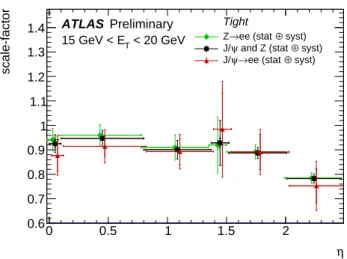
be referred to as “track quality” hereafter). The efficiencies are calculated as the ratio of the number of electrons passing a certain identification selection (numerator) to the number of electrons with a matching track passing the track quality requirements (denominator). For the identification efficiency measurements described in this note, two different decays of on-shell produced resonances are used: Z →eefor electrons withET>15 GeV andJ/ψ→eefor electrons with 7 GeV<ET<20 GeV. In the overlapping 15-20 GeV bin, results fromZ →eeandJ/ψ→eeare combined.
8.1. Tag-and-Probe withZ → ee Events
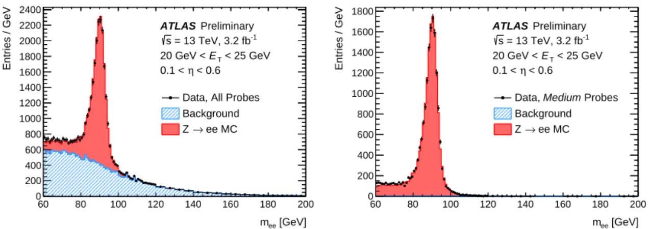
The tag-and-probe method is used withZ →eedecays to obtain a sample of unbiased electron candidates withET > 15 GeV. These electron candidates can then be used to determine the electron identification efficiency for the various operating points. As there is significant background contamination, particularly for ET < 25 GeV, the background needs to be statistically subtracted. To distinguish between signal electrons and background, two methods are used: the Zmass method uses the invariant mass of the tag-probe pair as the discriminating variable for background subtraction, while theZisomethod uses the calorimetric isolation distribution of the probe electron. These methods are treated as systematic variations on a single measurement.
8.1.1. Event Selection
Events are selected using a single electron trigger with anETthreshold of 24 GeV andMediumidentification requirements. These events are then required to have at least two reconstructed electron candidates in the central region of the detector,|η| < 2.47, with opposite charges. One of the two electrons, the tag, must haveET> 25 GeV, be matched to a trigger electron object within∆R<0.07, and be outside the transition region between the barrel and the endcap of the electromagnetic calorimeter, 1.37< |η| <1.52. The tag must satisfy an identification requirement, nominallyTight. The probes, meanwhile, are required to have ET >15 GeV and pass the track quality criteria. The discriminating variables for the probe are displayed in AppendixA(Figs. 18and19).
8.1.2. ZmassMethod
In the Zmass method, the identification efficiency is measured using the invariant mass spectrum of the tag-probe pairs in eachET andη bin of the probe electron. The signal is obtained from tag-probe pairs with an invariant massmee within 15 GeV of theZ boson nominal mass. The background is subtracted using templates which are constructed using probes that fail identification and isolation criteria, in order to model the background distribution with minimal contribution from signal electrons. Any residual signal contamination is estimated using simulated events and removed from the templates. The templates are then normalised to the data using the sidebands of the invariant mass distribution.
Different challenges exist for determining the numerator and the denominator for the ID efficiency in the Zmass method. For the denominator, there is a significant amount of background which must be properly estimated, and this is the primary source of systematic uncertainty in the measurement. For the numerator, meanwhile, the background contribution is typically several orders of magnitude smaller than the signal. However, as the majority of objects which pass the numerator selection are real electrons, there is significant signal contamination in the template normalisation regions at numerator level.
Thus, the calculation of the numerator and denominator is performed in different ways, to ensure that the challenges of each are properly addressed. Note that the same template distributions are used for both the numerator and the denominator, but the normalisation procedure differs between the two. Nominally, the normalisation region is the high invariant mass region 120 GeV< mee < 250 GeV.
As the invariant mass distribution of same-sign tag-probe pairs has less signal contamination than that of the opposite-sign tag-probe pairs, the numerator normalisation is performed using the same-sign sample.
At denominator level, however, the opposite-sign distribution must be used for the normalisation proced- ure as there is significant opposite-sign background present—and this is particularly important because some background processes such asW+jets predominantly contribute to the opposite-sign invariant mass distribution. Signal contamination at denominator level is accounted for, and estimated from the number ofTight events in the normalisation region, divided by theTight efficiency. This contamination is then subtracted from the normalization region.
Examples of the invariant mass distribution for the numerator and denominator for one bin in (ET,η) are shown in Fig.3.
To assess the systematic uncertainties, several variations are considered. Since the invariant mass distri- bution is used for the background subtraction, themee region of interest for determining the numerator and denominator is varied between mass windows of 10, 15, and 20 GeV on each side of the Z mass.
The tag identification criterion is varied by adding a calorimeter isolation requirement in addition to the nominalTight, or by loosening the tag requirement to Mediumwith calorimeter isolation. Finally, the background template is varied. ForET< 30 GeV, the background contamination is large, so the template normalisation is tested by using as a variation the invariant mass region 60 GeV< mee < 70 GeV instead of the nominal 120 GeV < mee < 250 GeV range. For ET > 30 GeV, the signal contamination in the templates is a larger concern as the background is much smaller. Moreover, there are far fewer events in this low mass region due to the kinematics, so only the 120 GeV < mee < 250 GeV normalisation is used. Instead, for ET > 30 GeV, a different template selection criterion is used as a variation. All possible combinations of these variations are used to determine the systematic uncertainties, as described in Sect.8.3. The template choice is found to be the most important systematic effect at lowET, while the variation on the invariant mass window is dominant at higherET.
8.1.3. ZisoMethod
The Ziso method is another method of background subtraction used to obtain the electron identification efficiency and scale-factors for electron energies of 15 GeV< ET < 200 GeV and |η| < 2.47 using the Z → eedecay. As a discriminating variable between signal and background, the calorimetric isolation Econe0.3
T of the probe is used. The calorimetric isolationEcone0.3
T follows the definition described in Sect.5 with a cone of∆R= 0.3 around the electron. Therefore, signal electrons should be accumulated around low values of the isolation variable whereas background should be found mainly at high values ofEcone0.3
T ,
allowing for the definition of a signal and background dominated region.
To estimate the background, a model is constructed representing the shape of the isolation distribution for background objects. For the construction of a background template, reconstructed probe electrons passing track quality criteria but failing the cut-basedLooseidentification or, alternatively, selected shower shape cuts, are selected. Furthermore, these probes are required to have the same charge as the tag electron. Real electrons passing the described background selection are estimated by applying the background selection to a Z → ee MC sample and are then subtracted from the background template. The Z → ee MC is
[GeV]
mee
60 80 100 120 140 160 180 200
Entries / GeV
0 200 400 600 800 1000 1200 1400 1600 1800 2000 2200 2400
Preliminary ATLAS
= 13 TeV, 3.2 fb-1
s
< 25 GeV ET
20 GeV <
< 0.6 η 0.1 <
Data, All Probes Background
ee MC
→ Z
[GeV]
mee
60 80 100 120 140 160 180 200
Entries / GeV
0 200 400 600 800 1000 1200 1400 1600 1800
Preliminary ATLAS
= 13 TeV, 3.2 fb-1
s
< 25 GeV ET
20 GeV <
< 0.6 η 0.1 <
Probes Medium Data, Background
ee MC
→ Z
Figure 3: Illustration of the background estimation using the Zmass method in the 20 GeV < ET < 25 GeV, 0.10< η <0.60 bin, at reconstruction level (left) and for probes passing theMediumidentification (right). Efficiencies are determined by taking the ratio of background-subtracted probes passing the likelihood identification over background-subtracted probes at reconstruction level. The simulatedZ →eesample is shown for illustration and is scaled to match the background-subtracted data in themeewindow.
/ 25 GeV
cone0.3
ET
0 0.5 1 1.5 2
Entries / 0.0625
1 10 102
103
104
ATLAS Preliminary = 13 TeV, 3.2 fb-1
s
Data, All Probes Background
ee MC
→ Z
ee MC+Background
→ Z
< 35 GeV ET
≤ 30 GeV
< -0.1 η
≤ -0.6
/ 25 GeV
cone0.3
ET
0 0.5 1 1.5 2
Entries / 0.0625
1 10 102
103
104
ATLAS Preliminary = 13 TeV, 3.2 fb-1
s
Probes Loose Data, Background
ee MC
→ Z
ee MC+Background
→ Z
< 35 GeV ET
≤ 30 GeV
< -0.1 η
≤ -0.6
Figure 4: Examples for denominator (left, reconstruction level) and numerator (right,Looseidentification) probe isolation distribution. The black dots represent data, the red dashed lines theZ → eeMC distribution. The light blue shaded area indicates the background model scaled to the tail of the data probe isolation distribution taking into account the signal contamination. The purple line represents the sum of theZ →eeMC and the background distribution which should describe the data points.
scaled to data by reconstructing theZ boson mass peak using oppositely charged tag-probe pairs passing a tight selection to reduce the background. The obtained background template is scaled to data in the background dominated tail of the probe isolation distribution, defined by Econe0.3
T /25 GeV > 0.5. An example of the probe isolation distribution and the obtained background template for one bin in (ET,η) is shown in Fig.4.
To evaluate the systematic uncertainties, several variations are considered. These include a modification of the tag-probe pair invariant mass window cut to 10 GeV or 20 GeV instead of 15 GeV around theZboson mass, as done in theZmassmethod. The tag selection is varied by adding a requirement on the calorimeter isolation (Econe0.3
T /25 GeV<0.3) to the requiredTightselection. In addition, different identification cuts are inverted to form two alternative background templates, and the definition of the background scaling
region is varied fromEcone0.3
T /25 GeV> 0.5 to Econe0.3
T /25 GeV > 0.4 or 0.6. A different choice of the isolation variable with a larger cone (Econe0.4
T ) around the probe electron allows for an evaluation of the uncertainty due to the choice of the discriminating variable. All possible combinations of the variations are considered. The main systematic effect originates from the background template variations.
8.2. Tag-and-Probe with J/ψ → eeEvents
J/ψ → eeevents are used to measure the identification efficiency of electrons with 7 GeV< ET < 20 GeV. At such low energies, the probe sample suffers from a significant background contamination, which can be estimated using the reconstructed di-electron invariant mass (mee) of the selected tag-probe pairs.
Furthermore, the J/ψ sample is composed of two contributions with significantly different electron identification efficiencies. The first contribution comes from theprompt productionof the J/ψmesons, which are produced directly in proton-proton collisions or in radiative decays of directly produced heavier charmonium states. The second contribution arises from thenon-prompt productionof the J/ψmesons, where the J/ψ come from b-hadron decays. The electrons from the decay of prompt J/ψ particles are expected to be more isolated, and therefore to have identification efficiencies closer to those of isolated electrons from other physics processes of interest in the same transverse momentum range, compared to those from non-prompt production.
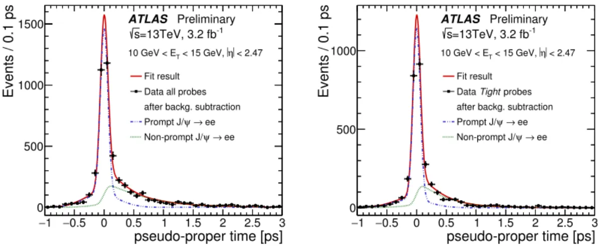
The two production modes can be distinguished by exploiting the long lifetime of b-hadrons, and the consequently displaced decay vertex of non-prompt J/ψ. This displacement can be estimated using the following variable, called pseudo-proper time:
τ= Lx y ·mJ/ψ
PDG
pJ/ψ
T
, (3)
whereLx yis the distance between theJ/ψvertex and the primary vertex in the transverse plane, andmJ/ψ
PDG
andpJ/ψ
T are the mass and the reconstructed transverse momentum of the J/ψmeson, respectively.
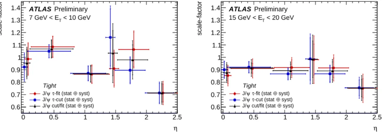
Both methods of efficiency measurement described in Ref. [3] have been used for these measurements.
The key difference between the two methods is in the different approach for separating between prompt and non-prompt components using the pseudo-proper time distribution. The first method is calledJ/ψ τ- cut and applies an explicit cut on the τ distribution to enrich the selected sample with prompt J/ψ. The residual fraction of the non-prompt component is determined from MC simulation and the ATLAS measurement of the non-prompt fraction inJ/ψ →µµevents [20]. TheJ/ψ τ-fit method utilises the full sample and extracts the non-prompt fraction by fitting the pseudo-proper time distribution both before and after applying the identification cuts.
8.2.1. Event Selection
The baseline event selection is the same for both theJ/ψ τ-cut andJ/ψ τ-fit methods. Events are required to have at least two electrons with ET > 5 GeV and pseudorapidity |η| < 2.47. At least one of five dedicatedJ/ψtwo-object triggers must fire in the event. Each of these triggers requires a likelihoodTight trigger electron identification andETabove certain threshold for one trigger object, while only demanding the electromagnetic clusterETto be higher than some other threshold for the second object. Tag electron candidates must match a Tight trigger electron object within ∆R < 0.07 and satisfy the offline Tight