ATLAS NOTE ATL-CONF-2016-065

A TLAS-CONF-2016-065 08 August 2016

ATLAS NOTE

ATL-CONF-2016-065

5th August 2016

Measurement of the cross-section of the production of a W boson in association with a single top quark

with ATLAS at √

s = 13 TeV

The ATLAS Collaboration

Abstract

The inclusive production cross-section for the associated production of a W boson and top quark is measured using data from proton–proton collisions at

√ s = 13 TeV. The dataset corresponds to an integrated luminosity of 3 . 2 fb ^{− 1} , and was collected in 2015 by the ATLAS detector at the Large Hadron Collider at CERN. Events are separated into signal and control regions based on their jet multiplicity and the number of jets that are identified as containing b hadrons. The W t signal is then separated from the t¯ t background using boosted decision tree discriminants in two regions. The cross-section is extracted by fitting templates to the data distributions, and is measured to be σ _{W t} = 94 ± 10 ( stat .) ⁺²⁸ ₋

23 ( syst .) pb. The measurement is in agreement with the Standard Model prediction.

© 2016 CERN for the benefit of the ATLAS Collaboration.

Reproduction of this article or parts of it is allowed as specified in the CC-BY-4.0 license.

1 Introduction

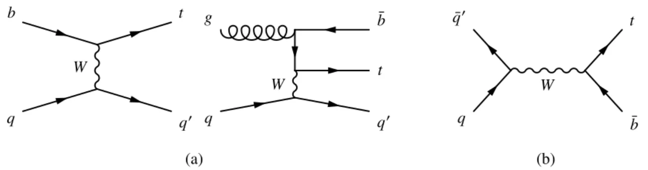
Top quarks can be produced singly via electroweak interactions involving a W tb vertex. In the Standard Model (SM), single top quark production proceeds via three channels at leading order (LO), represented in Figs. 1 and 2: production in association with a W boson ( W t ), the t channel and the s channel. At the Large Hadron Collider (LHC), the W t channel is the second largest mode in terms of production cross-section, following the dominant t -channel mode. The W t channel represents approximately 24 % of the total single top quark production rate at

√ s = 13 TeV, making it experimentally accessible for detailed measurements.

b t

W ⁻

W ⁺ g

b

` ⁺ ν b

` ⁻ ν ¯

Figure 1: A representative leading order Feynman diagram of the production of a single top quark in the W t channel and the subsequent leptonic decay of both the W boson and top quark.

W

q b

q ⁰ t

W q

g

q ⁰ t b ¯

W q

q ¯ ⁰

b ¯ t

(a) (b)

Figure 2: Representative leading order Feynman diagrams of the production of a single top quark in (a) the t channel and (b) the s channel.

The cross-section for each of the three single top quark production channels is proportional to the coupling between the W boson and the top quark. This coupling is parameterised by the relevant Cabibbo–

Kobayashi–Maskawa (CKM) matrix element V _{t b} and form factor f _LV [1–3] such that the proportionality is given by | f _LV V _{t b} | ² [4, 5]. Single top quark production therefore presents an opportunity for precision testing of the structure of the SM, as well as probing classes of new physics models that can affect the W tb vertex. In contrast to the t and s channels, which are sensitive to both the existence of four fermion operators and corrections to the W tb vertex, the W t channel only depends on the latter; it is therefore important to study this channel separately to provide a comparison with the other channels [6, 7].

The cross-section of the W t channel at next-to-leading order (NLO) with next-to-next-to-leading logar-

ithmic (NNLL) soft-gluon corrections is calculated as σ _theory = 71 . 7 ± 1 . 8 ( scale ) ± 3 . 4 ( PDF ) pb [8],

assuming a top quark mass of 172.5 GeV at centre-of-mass energy of 13 TeV. The first uncertainty ac-

counts for the renormalisation and factorisation scale variations (from 1 / 2 to 2 times the top quark mass),

while the second uncertainty originates from the 90 % confidence level uncertainties in the MSTW2008

NLO parton distribution function (PDF) sets [9].

The W t channel was not accessible at the Tevatron due to its small cross-section. At the LHC, however, evidence for this process with 7 TeV collision data was presented by the ATLAS Collaboration [10]

and by the CMS Collaboration [11]. With 8 TeV collision data, observations were made by the CMS Collaboration [12] and the ATLAS Collaboration [13]. Both cross-section measurements agreed well with theoretical predictions.

This note describes a measurement of the inclusive cross-section of the W t process using 3 . 2 fb ^{− 1} of

√ s =13 TeV proton–proton ( pp ) collisions recorded by the ATLAS detector in 2015. The measurement is made using events containing at least one b -tagged jet and exactly two oppositely-charged leptons in the final state, where a lepton ( ` ) is defined to be either an electron ( e ) or a muon ( µ ), whether produced directly from the decay of a W boson or from the decay of an intermediate τ lepton. The W t signal enters this final state when the top quark decays into a W boson and a quark (which is a b quark in almost all such decays), with both W bosons subsequently decaying into a neutrino and a lepton, as depicted in Fig. 1. A minimal selection is applied to reduce background contributions from Z/γ ^∗ +jets (hereafter called Z +jets) events, diboson events, and events containing leptons that are misidentified or arising from the decay of hadrons. A boosted decision tree (BDT) analysis is performed to construct discriminants capable of separating the W t signal from the dominant top quark pair ( t¯ t ) background, and these discriminants are used in a profile likelihood fit to extract the W t cross-section.

The measurement technique is similar to that employed in the corresponding 8 TeV ATLAS measure- ment [13]. The most significant changes include modifications to the BDT training and the binning of the likelihood fit (discussed in Sect. 6 and Sect. 8 respectively), and an optimisation of cuts to more effectively reject Z +jets and other small backgrounds (discussed in Sect. 5).

2 The ATLAS detector

The ATLAS detector [14] at the LHC covers nearly the entire solid angle1 around the collision point, and consists of an inner tracking detector (ID) surrounded by a thin superconducting solenoid magnet producing a 2 T axial magnetic field, electromagnetic (EM) and hadronic calorimeters, and an external muon spectrometer (MS). The ID consists of a high-granularity silicon pixel detector and a silicon microstrip tracker, together providing precision tracking in the pseudorapidity range |η | < 2 . 5, complemented by a transition radiation tracker providing tracking and electron identification information for |η| < 2 . 0. The innermost pixel layer, the insertable B-layer, was added between Run-1 and Run-2 of the LHC, at an average radius of only 33 mm around a new, thinner, beam pipe [15]. A lead liquid-argon (LAr) electromagnetic calorimeter covers the region |η | < 3 . 2, and hadronic calorimetry is provided by steel/scintillating tile calorimeters within |η | < 1 . 7 and copper/LAr hadronic endcap calorimeters in the range 1 . 5 < |η| < 4 . 9.

The MS consists of precision tracking chambers covering the region |η | < 2 . 7, and separate trigger chambers covering |η | < 2 . 4. A two-level trigger system, using a custom hardware level, followed by a software-based level, is used to reduce the collision rate from 40 MHz to a maximum of around 1 kHz for offline storage.

1

ATLAS uses a right-handed coordinate system with its origin at the nominal interaction point (IP) in the centre of the detector and the z -axis along the beam pipe. The x -axis points from the IP to the centre of the LHC ring, and the y -axis points upward. Cylindrical coordinates (r, φ) are used in the transverse plane, φ being the azimuthal angle around the z -axis. The pseudorapidity is defined in terms of the polar angle θ as η = − ln tan (θ/ 2 ) , while the rapidity is defined in terms of particle energies and the z -component of particle momenta as y = ( 1/2 ) ln

(E + p

)/(E − p

)

.

3 Data and simulated samples

The data events analysed in this note correspond to an integrated luminosity of 3 . 2 fb ^{− 1} , collected from the operation of the LHC in 2015 at

√ s = 13 TeV, with bunch spacing 25 ns and an average number of collisions per bunch crossing hµi around 40. They are required to be recorded in periods where all detector systems are flagged as operating normally. Additionally, individual events identified as containing corrupted data are rejected.

Monte Carlo (MC) simulation samples are used to estimate the efficiency to reconstruct signal and background events, train and test BDTs, estimate systematic uncertainties, and validate the analysis tools.

The nominal samples (used for estimating the central values for efficiencies and background templates) were simulated with a full ATLAS detector simulation [16] implemented in Geant 4 [17]. Many of the samples used in the evaluation of systematic uncertainties were instead produced using Atlfast2 [18], which differs from the full simulation in that the ATLAS calorimeters and their responses were simulated using a faster approximation. Pile-up (additional pp collisions in the same or neighbouring bunch crossing as the triggered event) was included in the simulation by overlaying collisions with the soft QCD processes of Pythia 8.186 [19] using the A2 [20] set of tuned parameters and the MSTW2008LO PDF set. Events were generated with a pre-defined distribution of the expected number of interactions per bunch crossing, then reweighted to match the actual observed data conditions. The top quark mass ( m _top ) was set to 172.5 GeV in all samples used in this analysis, and the W → `ν branching ratio was set to 0 . 1080.

For the generation of W t and t¯ t event samples [21], the Powheg-Box v1 (v2 for t t ¯ ) [22–26] generator with the CT10 PDF sets [27] in the matrix element calculations is used. For these processes, top quark spin correlations are preserved. The parton shower, fragmentation, and underlying event were simulated using Pythia 6.428 [28] with the CTEQ6L1 PDF sets [29] and the corresponding Perugia 2012 tune (P2012) [30]. The EvtGen v1.2.0 program [31] was used for properties of the bottom and charmed hadron decays. The renormalisation and factorisation scales are set to m _top for the W t process and q

m ² _t + p _T (t) ² for t¯ t . The diagram removal (DR) scheme [32], in which all NLO diagrams that overlap with the t t ¯ definition are removed from the calculation of the W t amplitude, was employed to handle interference between W t and t¯ t diagrams, and is applied to the W t sample.

Additional W t samples were generated to evaluate major sources of systematic uncertainties. A W t sample using the diagram subtraction (DS) scheme instead of DR, where a gauge-invariant subtraction term modifies the NLO W t cross-section to locally cancel the double-resonant t¯ t contribution [32], was otherwise generated in the same way as the nominal sample. Another sample generated with MadGraph5_aMC@NLO [33] (instead of the Powheg-Box) interfaced with Herwig++ 2.7.1 [34] using Atlfast2 fast simulation is used to evaluate uncertainties associated with the modelling of the matrix element generator, and a sample generated with Powheg-Box interfaced with Herwig++ (instead of Pythia 6) is used to evaluate uncertainties associated with the parton shower and hadronisation models.

In both cases the UE-EE-5 set of tuned parameters of Ref. [35] was used for the underlying event, and

EvtGen v1.2.0 was used for describing properties of the bottom and charmed hadron decays. Finally, in

order to evaluate uncertainties arising from additional QCD radiation in the W t events, a pair of samples

were generated with Powheg-Box interfaced with Pythia 6 using Atlfast2 and the P2012 set of tuned

parameters with higher and lower radiation relative to the nominal set, together with varied renormalisation

and factorisation scales. In these samples the resummation damping factor is doubled in the case of higher

radiation.

Additional t¯ t samples to evaluate major sources of systematic uncertainties were generated. As with the additional W t samples, these are used to evaluate the uncertainties associated with the matrix element generator (a sample produced using Atlfast2 fast simulation with MagGraph5_aMC@NLO interfaced with Herwig++ 2.7.1), parton shower and hadronisation models (a sample produced using Atlfast2 with Powheg-Box interfaced with Herwig++ 2.7.1) and additional QCD radiation (a pair of samples produced using full simulation with the P2012 higher and lower radiation-varied sets of parameters, as well as with varied renormalisation and factorisation scales).

Samples used to model the Z +jets background [36] were simulated with Sherpa 2.1.1 [37]. Matrix elements were calculated for up to two partons at NLO and four partons at LO using the Comix [38] and OpenLoops [39] matrix element generators and merged with the Sherpa parton shower [40] using the ME+PS@NLO prescription [41]. The CT10 PDF set was used in conjunction with Sherpa parton shower tuning, with a generator-level cutoff of m _`` > 40 GeV applied.

Diboson processes with four charged leptons, three charged leptons and one neutrino, or two charged leptons and two neutrinos [42] were simulated using the Sherpa 2.1.1 generator. The matrix elements contain all diagrams with four electroweak vertices. They were calculated for up to one (two or four charged leptons) or zero partons (three charged leptons) at NLO and up to three partons at LO using the Comix and OpenLoops matrix element generators and merged with the Sherpa parton shower using the ME+PS@NLO prescription [41]. The PDF set used was CT10 with dedicated parton shower tuning.

Finally, the very small W +jets contribution is simulated using Powheg-Box v2 interfaced to the Py- thia 8.186 [19] parton shower model. The CT10 PDF set is used in the matrix element. The AZNLO [43]

tune is used, with PDF set CTEQ6L1, for the modelling of non-perturbative effects, and the EvtGen v1.2.0 program is used for describing properties of the bottom and charmed hadron decays.

4 Object selection

Electron candidates are reconstructed from energy deposits in the EM calorimeter associated with ID tracks [44]. The clusters are required to be in the |η | < 2 . 47 region, with the transition region between the barrel and end-cap EM calorimeters, 1 . 37 < |η | < 1 . 52, excluded. The candidate electrons are required to have transverse energy p _T > 20 GeV. Further requirements on the electromagnetic shower shape, calorimeter energy to tracker momentum ratio, and other discriminating variables are combined into a likelihood-based object quality selection [44], optimised for strong background rejection. Electrons are further required to be isolated based on ID tracks and topological calorimeter clusters [45], with an isolation efficiency of 90 ( 99 ) % for p _T = 25 ( 60 ) GeV.

Muon candidates are identified by matching MS segments with ID tracks [46]. The candidates must pass quality selections based upon requirements on hits in MS subsystems and the compatibility between ID and MS momentum measurements to remove fake muon signatures. Furthermore, they must have p _T > 20 GeV as well as | η| < 2 . 5 to ensure they are within the coverage of ID. The isolation requirement is imposed based on ID tracks and topological calorimeter clusters, and results in an isolation efficiency of 90(99) % for p _T = 25(60) GeV.

Jets are reconstructed from topological calorimeter clusters using the anti- k _t algorithm [47, 48] with a

radius parameter of 0.4. They are required to be within the range p _T > 25 GeV and |η | < 2 . 5. To

suppress pile-up, a discriminant called the jet-vertex-tagger (JVT) is constructed using a two dimensional

likelihood method [49]. For jets with p _T < 60 GeV and |η | < 2 . 4 a JVT requirement corresponding to a 92 % efficiency and 2 % fake rate is imposed.

Jets containing b hadrons ( b jets) are tagged using a multivariate discriminator which exploits the long lifetime and large invariant mass of b hadron decay products relative to c hadrons and unstable light hadrons [50]. The discriminator is calibrated to achieve a 77 % b -tagging efficiency and rejection factor of about 4.5 against jets containing charm quarks ( c jet) and 140 against light-quark and gluon jets in a sample of simulated t¯ t events [51]. The b -tagging efficiency in simulation is corrected to the efficiency in data [52].

The missing transverse momentum vector is calculated as the negative vectorial sum of the momenta in the transverse plane of particles in the event. Its magnitude E ^miss

T is a measure of the transverse momentum imbalance, primarily due to neutrinos that escape detection. In addition to the identified jets, electrons and muons, a track-based soft term is included in the E ^miss

T calculation by considering tracks associated with the hard scattering vertex in the event which are not associated with an identified jet, electron, or muon [53, 54]. The E ^miss

T is sensitive to energy losses due to detector inefficiencies and resolution that lead to the mis-measurement of the true E _T of the final interacting objects.

To avoid cases where the detector response to a single physical object is reconstructed as two separate final state objects, several steps are followed to remove such overlaps. First, an electron sharing an ID track with a muon is removed to avoid cases where a muon mimics an electron through radiation of a hard photon.

Next, the closest jet to each electron within an y − φ cone of size ∆R _y,φ = p

( ∆ y) ² + ( ∆φ) ² = 0 . 2 is removed to reduce the probability of electrons being reconstructed as jets. Next, electrons with a distance

∆R _y,φ < 0 . 4 from any of the remaining jets are removed to reduce backgrounds from non-prompt, non- isolated electrons originating from heavy flavour hadron decays. Jets with fewer than three tracks and distance ∆R _y,φ < 0 . 4 from a muon are then removed to reduce fake jets from muons depositing energy in the calorimeters. Finally, muons with a distance ∆R _y,φ < 0 . 4 from any of the surviving jets are removed to avoid contamination of non-prompt muons from heavy flavour hadron decays.

5 Event selection and background estimation

Events are required to pass a single electron or muon trigger which is designed to select events containing a high- p _T , well-identified charged lepton. The triggers impose a lower p _T requirement at 20 GeV for muons and 24 GeV for electrons, and also have requirements on the lepton quality and isolation. These are complemented by triggers with higher p _T thresholds and relaxed isolation and identification requirements to ensure maximum efficiency at higher lepton p _T . At least one jet with p _T > 25 GeV is required in each event, motivated by the jet arising from the top quark decay in the W t signal process. Events are then required to contain exactly two charged leptons (i.e. electrons or muons) of opposite charge with p _T > 20 GeV, satisfying the object requirements described in Sect. 4; events with a third lepton with p _T > 20 GeV are rejected. At least one lepton must have p _T > 25 GeV, and at least one of the selected electrons (muons) must be matched within a ∆R cone of size 0 . 07 (0 . 1) to the electron (muon) selected online by the corresponding trigger. Thus events must have one high- p _T lepton due to trigger requirements, while the additional lepton p _T threshold was chosen to be as low as necessary to efficiently select signal events.

In simulated events, information from the event generator record is used to identify events in which any

selected lepton does not originate promptly from the hard scatter process. These fake leptons arise from

processes such as the decay of a b hadron, photon conversion or hadron misidentification, and are identified when the electron or muon does not originate from the decay of a W or Z boson (or a τ lepton itself originating from a W or Z ). Events with a selected lepton which is fake are themselves labelled as fake and are treated as a contribution to the background.

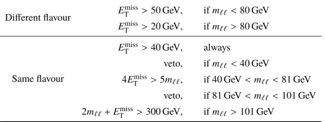
After this selection has been made, a further set of requirements is imposed with the aim of reducing the contribution from the Z +jets, diboson and fake lepton backgrounds; the resultant sample is intended to consist almost entirely of W t signal and t¯ t background, which will be subsequently separated by the BDT analysis. Events in which the two leptons have the same flavour and an invariant mass consistent with having originated from a Z boson (81 < m _{``</sub> < 101 GeV) are vetoed, as well as those with a low invariant mass m <sub>``} < 40 GeV. Further requirements on E ^miss

T and m _`` are chosen based on the flavour of the selected leptons (as shown in Table 1). Events with different-flavour leptons are required to have E ^miss

T > 20 GeV, with the requirement raised to E ^miss

T > 50 GeV when the dilepton invariant mass satisfies m _`` < 80 GeV. All events with same-flavour leptons must satisfy E ^miss

T > 40 GeV. For same-flavour events, the Z +jets background is concentrated in a region of the m _`` - E ^miss

T plane corresponding to values of m _`` near the Z mass, and towards low values of E ^miss

T . Therefore, a triangular selection in E ^miss

T and

m _{``</sub> is used to remove these backgrounds: events with 40 GeV < m <sub>``} < 81 GeV are required to satisfy 4 × E ^miss

T > 5 × m _{``</sub> while events with m <sub>``} > 101 GeV are required to satisfy 2 × m _`` + E ^miss

T > 300 GeV.

The requirements for the same- and different-flavour events are chosen separately due to the kinematically different processes contributing to the Z +jets background, namely Z → ee/µµ in same-flavour events and Z → ττ in different-flavour events.

The sample of selected events is divided into regions based on the number of jets and b -tagged jets. At LO, the signal process results in a final state with one b jet arising from the top quark decay, and no additional jets, while the t t ¯ process results in two b jets from the top quark decays. Events with additional jets are also studied since the underlying event, QCD radiation and other effects may produce additional jets in signal events.

According to these expected final states, two signal regions are defined by the presence of exactly one b -tagged jet and either zero (denoted 1j1b ) or one (denoted 2j1b ) additional jet. A t¯ t -enriched control region is defined by the presence of exactly two jets, which are both b -tagged (denoted 2j2b ). This control region is used to constrain the t t ¯ background normalisation, and is expected to contain only a small ( < 1 %) proportion of signal events. These three regions — 1j1b , 2j1b and 2j2b — are called the fit regions, as they are used in the simultaneous fit procedure described in Sect. 8. Event yields for each fit region are presented in Sect. 9. Two additional regions, in which events are required to contain one (denoted 1j0b ) or two (denoted 2j0b ) jets but no b -tagged jets are used to validate the description of the data by the simulation. The expected event yields (from MC simulation) for signal and backgrounds with their total systematic uncertainties, as well as the number of observed events in the data in the five regions are shown in Fig. 3.

6 Separation of signal from background

After the event selection is performed, the data sample consists primarily of t¯ t with a significant number

of W t signal events (see for example Fig. 3). As there is no single observable that clearly discriminates

between the W t signal and the t¯ t background, several observables are combined into a single powerful

discriminator using a BDT technique [55]. A collection of decision trees is created that weakly separates

events into signal and background based on a number of binary decisions considering a single observable

Table 1: Summary of event selection criteria used in the analysis.

At least one jet with p _T > 25 GeV

Exactly two leptons of opposite charge with p _T > 20 GeV

At least one lepton with p _T > 25 GeV, veto if third lepton with p _T > 20 GeV At least one lepton matched to the trigger object

Different flavour

E ^miss

T > 50 GeV, if m _`` < 80 GeV E ^miss

T > 20 GeV, if m _`` > 80 GeV

Same flavour

E ^miss

T > 40 GeV, always

veto, if m _`` < 40 GeV 4 E ^miss

T > 5 m _{``</sub> , if 40 GeV < m <sub>``} < 81 GeV veto, if 81 GeV < m _{``</sub> < 101 GeV 2 m <sub>``} + E ^miss

T > 300 GeV, if m _`` > 101 GeV

Events

2000 4000 6000 8000 10000

12000 ATLAS Preliminary = 13 TeV, 3.2 fb

s

Data 2015 Wt

t t Z+jets Others Total syst.

Regions

1j1b 2j1b 2j2b 1j0b 2j0b

Data/Pred. 0.6 0.8 1 1.2 1.4

Figure 3: Expected event yields for signal and backgrounds with their total systematic uncertainty (discussed in

Sect. 8) and the number of observed events in the data are shown in the three fit regions ( 1j1b , 2j1b , and 2j2b )

and the two additional regions ( 1j0b and 2j0b ). The signal and backgrounds are normalised to their theoretical

predictions, and the error bands represent the total systematic uncertainties on the Monte Carlo predictions. The

upper panels give the yields in number of events per bin, while the lower panels give the ratios of the numbers of

observed events to the total prediction in each bin.

at a time. A boosting algorithm is then used to assign weights to each tree such that the ensemble of weak classifiers performs as a strong classifier [56]. In this analysis, the BDT implementation is provided by the tmva package [57], using the GradientBoost algorithm for boosting.

Separate BDTs are prepared for the analysis regions 1j1b and 2j1b . No BDT is constructed for the 2j2b region in order to reduce the impact of t t ¯ modelling uncertainties, which are found to be most significant in this region. The BDTs are optimised to distinguish between W t and t¯ t by using the nominal W t sample, the DS W t sample and the nominal t¯ t sample; for each sample, half of the events are used for training while the other half is reserved for testing. For each region, a large list of variables is prepared for the BDT. An optimisation procedure is then carried out in each region to select a subset of input variables and a set of BDT parameters (such as the number of trees in the ensemble and the maximum depth of the individual decision trees). The optimisation is designed to provide the best separation between the W t signal and t¯ t background while avoiding sensitivity to statistical fluctuations in the training sample.

This latter requirement is enforced by conducting a Kolmogorov–Smirnov (KS) statistical test [58], which compares the BDT response in the training sample to that in the reserved test sample, requiring that the KS test statistic be greater than 0.1.

The variables considered are derived from the kinematic properties of subsets of the selected physics objects (defined in Sect. 4) present in the event. For a set of objects o ₁ . . . o _n : p ^sys

T ( o ₁ . . . o _n ) is the magnitude of the vectorial sum of transverse momenta; H _T ( o ₁ . . . o _n ) is the scalar sum of transverse momenta; P

E _T is the scalar sum of the transverse energy of all objects which contribute to the E ^miss

T

calculation; σ (p ^sys

T ) is the ratio of p ^sys

T to (H _T + P

E _T ) ; m ( o ₁ . . . o _n ) is the invariant mass; m _T ( o ₁ . . . o _n ) is the transverse mass (i.e. the invariant mass of ( o _{1 , T} . . . o _nT each projected into the transverse plane); and E/m ( o ₁ . . . o _n ) is the ratio of energy to invariant mass. For two systems of objects s ₁ and s ₂ : ∆R(s ₁ , s ₂ ) is the separation in φ - η space; ∆p _T (s ₁ , s ₂ ) is the p _T difference; ∆φ( s ₁ , s ₂ ) is the φ difference; and C(s ₁ , s ₂ ) , the centrality, is the ratio of the scalar sum of p _T to the sum of energy.

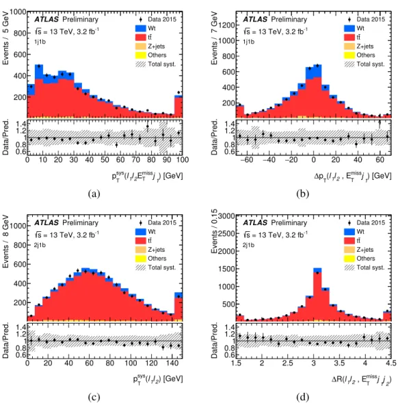
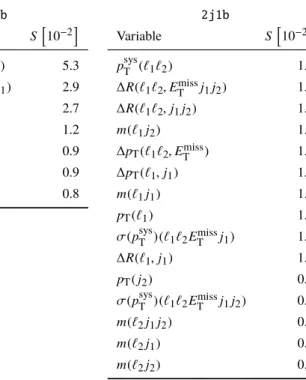
The final selection of input variables used in each BDT is listed in Table 2 along with the separating power of each variable2. In order to check that the variables and their correlations in W t signal and the background events are well modelled by simulation, the distributions of these variables and the BDTs are compared between the MC expectations and the observed data. The distributions of the two most powerful variables in each region are shown in Fig. 4. The MC predictions describe the data well, within the total systematic uncertainties.

7 Systematic uncertainties

The experimental sources of uncertainty include the measurement of the luminosity, lepton efficiency scale factors, lepton energy scale and resolution, E ^miss

T soft term calculation, jet energy scale and resolution, and the b -tagging efficiency. Among these, the dominant sources of uncertainty are due to the determination of the jet energy scale (JES) and jet energy resolution. The JES uncertainty [45] is split into several orthogonal components representing independent effective uncertainties using in situ techniques (JES Eff.), model uncertainties (such as flavour composition, η intercalibration model), and other systematics on the JES

2

The separating power, S , is a measure of the difference between probability distributions of signal and background in the variable, and is defined as

< S

>= 1 2

Z (Y

(y) − Y

(y))

(Y

(y) + Y

( y)) dy

where Y

( y) and Y

( y) are the signal and background probability distribution functions of each variable y , respectively.

Events / 5 GeV

200 400 600 800 1000

Data 2015 Wt

t t Z+jets Others Total syst.

ATLAS Preliminary = 13 TeV, 3.2 fb-1

s 1j1b

) [GeV]

j

E

l

l

( p

0 10 20 30 40 50 60 70 80 90 100 Data/Pred. 0.6 0.8 1 1.2 1.4

Events / 7 GeV

200 400 600 800 1000

1200

t t Z+jets Others Total syst.

ATLAS Preliminary = 13 TeV, 3.2 fb-1

s 1j1b

) [GeV]

j

, E

l

l

(

∆ p

− 60 − 40 − 20 0 20 40 60 Data/Pred. 0.6 0.8 1 1.2 1.4

(a) (b)

Events / 8 GeV

200 400 600 800

1000

Wt t t Z+jets Others Total syst.

ATLAS Preliminary = 13 TeV, 3.2 fb-1

s 2j1b

) [GeV]

l

l

( p

0 20 40 60 80 100 120 140

Data/Pred. 0.6 0.8 1 1.2 1.4

Events / 0.15

500 1000 1500 2000 2500

3000

Wt t t Z+jets Others Total syst.

ATLAS Preliminary = 13 TeV, 3.2 fb-1

s 2j1b

2

)

1

j

miss

j , E

l

l

∆ R(

1.5 2 2.5 3 3.5 4 4.5

Data/Pred. 0.6 0.8 1 1.2 1.4

(c) (d)

Figure 4: Distributions of the two most powerful BDT input variables in each fit region: in the 1j1b region (a) p

T

(`

`

E

T

j

) and (b) ∆p

(`

`

E

T

j

) ; in the 2j1b region (c) p

T

(`

, `

) and (d) ∆R(`

`

, E

T

j

j

) . The

signal and backgrounds are normalised to their theoretical predictions, and the error bands represent the total

systematic uncertainties on the Monte Carlo predictions. The first and last bins of each distribution contain overflow

events. The upper panels give the yields in number of events per bin, while the lower panels give the ratios of the

numbers of observed events to the total prediction in each bin.

Table 2: The variables used in each BDT and their separating powers (a measure of the difference between probability distributions of signal and background in the variable, denoted S ). The variables are derived from the four-vectors of the leading (sub-leading) lepton `

( `

), the leading (sub-leading) jet j

( j

) and E

T

.

1j1b

Variable S f

10

g

p

T

(`

`

E

T

j

) 5.3

∆p

(`

`

, E

T

j

) 2.9

P E

2.7

∆p

(`

`

, E

T

) 1.2

p

T

(`

E

T

j

) 0.9

C(`

`

) 0.9

∆p

(`

, E

T

) 0.8

2j1b

Variable S f

10

g

p

T

(`

`

) 1.7

∆R(`

`

, E

T

j

j

) 1.7

∆R(`

`

, j

j

) 1.5

m(`

j

) 1.4

∆p

(`

`

, E

T

) 1.4

∆p

(`

, j

) 1.4

m(`

j

) 1.3

p

(`

) 1.3

σ( p

T

)(`

`

E

T

j

) 1.2

∆R(`

, j

) 1.2

p

( j

) 0.9

σ( p

T

)(`

`

E

T

j

j

) 0.9

m(`

j

j

) 0.3

m(`

j

) 0.3

m(`

j

) 0.1

determination (such as pileup jet area, ρ ) derived using

√ s = 13 TeV data. The most significant JES uncertainty components for this analysis are the in situ calibration and the flavour composition uncertainty.

The jet energy resolution uncertainty estimate [45] is based on comparisons of simulation and data using in situ studies with Run-1 data. These studies are then cross-calibrated and checked to confirm good agreement with Run-2 data. As discussed in Sect. 4, the E ^miss

T calculation includes contributions from hard sources, including leptons and jets, in addition to soft terms which arise primarily from low- p _T pileup jets and underlying event activity. The uncertainty associated with the hard terms is propagated from the corresponding jet and lepton scale and resolution uncertainties, and is classified together with the uncertainty on the hard objects. The uncertainty associated with the soft term is calculated by comparing the simulated scale and resolution to that in data, including differences in uncertainties due to model dependence. A 2.1% uncertainty is assigned to the integrated luminosity determination for 2015 data.

It is derived, following a methodology similar to that detailed in Ref. [59], from a calibration of the luminosity scale using x – y beam-separation scans performed in August 2015.

Uncertainties on the scale factors to correct the b -tagging efficiency in simulation to the efficiency in data are assessed using independent eigenvectors for the efficiency of b jets, c jets, light-parton jets, and two extrapolation uncertainty factors. These b -tagging uncertainties are determined with

√ s = 8 TeV data, then extrapolated to and checked on

√ s = 13 TeV data.

Uncertainties stemming from theoretical models are evaluated by comparing a set of predicted distributions

produced under different assumptions and applying the difference observed as a weight to the nominal

W t or t¯ t distribution. The main uncertainties are due to the NLO matrix element (ME) generator,

parton shower and hadronisation (PS) generator, initial- and final-state radiation (I/FSR) tuning and the

PDF. The NLO matrix element uncertainty is evaluated by comparing two NLO matching methods: the predictions of Powheg with MadGraph5_aMC@NLO, both interfaced with Herwig++. The parton shower and hadronisation uncertainty is estimated by comparing Powheg interfaced with either Pythia 6 or Herwig++. The matrix element generator uncertainty is treated as uncorrelated between the W t and t t ¯ processes, while the parton shower generator uncertainty is treated as correlated. The I/FSR tuning uncertainty is evaluated by taking half of the difference between samples with Powheg interfaced with Pythia 6 tuned with either more or less radiation, and is uncorrelated between the W t and t¯ t processes due to the different set of parameters adjusted in each sample. The choice of scheme to account for the interference between the W t and t¯ t processes constitutes another major source of systematic uncertainty for the signal modelling, and it is estimated by comparing the diagram removal scheme samples and the diagram subtraction scheme samples, both generated with Powheg+Pythia 6. The uncertainty due to the choice of parton distribution function (PDF) is evaluated using the PDF4LHC15 combined PDF set [60]. The difference between the central CT10 [27] prediction and the central PDF4LHC15 prediction (PDF central value) is taken and symmetrised together with the internal uncertainty set provided with PDF4LHC15. For t¯ t and W t modelling, the NLO matrix element model, parton shower model, and PDF uncertainties are evaluated using fast simulated samples, and for W t fast simulation is also used for I/FSR.

In each case where results from two samples must be compared, fast simulated samples are only compared to other fast simulated samples.

Additionally, normalisation uncertainties of 100 % are assumed for the fake and non-prompt backgrounds.

The Z +jets backgrounds with one b -tagged jet are assigned a 50 % uncertainty, while a 100 % uncertainty is assumed on Z +jets events with two b -tagged jets. Diboson backgrounds are assigned an uncertainty of 25 % to cover the difference in predictions between the Sherpa and Powheg generators. These uncertainties are treated as uncorrelated across the various regions of jet and b -tagged jet multiplicity.

Table 3 gives a breakdown of uncertainties on the final fitted cross-section.

8 Extraction of signal cross-section

The W t cross-section is extracted from the data using a profile likelihood fit that combines inputs from several signal and control regions to constrain backgrounds and systematic uncertainties. The fit uses the HistFitter [61] software framework, which is in turn built on the HistFactory , RooStats , and RooFit [62] frameworks. These tools assist in implementing a template profile likelihood fit with multiple signal and control regions.

The fit uses the binned BDT response in two of the three fit regions ( 1j1b and 2j1b ) and a single bin in the 2j2b region to construct templates for the W t signal and each modelled background ( t¯ t , Z +jets, diboson, fake and non-prompt leptons). For each signal and background template, an additional template is constructed for each systematic variation discussed in Sect. 7. Systematic uncertainties are considered by allowing Gaussian-constrained nuisance parameters to deform fit templates to their

± 1 σ variations while simultaneously varying the normalisation of the templates. The normalisation of the t¯ t background, µ _{t t ¯} , is also determined in the fit by assigning an unconstrained parameter to the t¯ t normalisation. Other backgrounds are constrained within their systematic uncertainties by Gaussian- constrained nuisance parameters, and all templates are affected by the overall luminosity uncertainty.

A global likelihood function is constructed to describe the agreement between data and prediction as a

function of the parameter of interest, namely the W t signal strength µ _{W t} , and a list of nuisance parameters

each describing the influence of a different source of systematic uncertainty. The W t cross-section and its uncertainty are extracted from the fitted value of µ _{W t} , with a value of unity corresponding to the predicted NLO+NNLL σ _theory value.

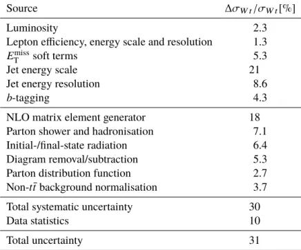
Table 3: Relative uncertainties on the W t cross-section. These are evaluated by fixing each uncertainty parameter to its post-fit ± 1 σ uncertainties, re-fitting, and assessing the change in the signal strength. Due to correlations between parameters, the individual uncertainty categories are not expected to add up to the total systematics. The statistical uncertainty is evaluated by fitting without any nuisance parameters corresponding to systematic uncertainty in the fit, and the total systematics is evaluated by subtracting the statistical uncertainty from the total uncertainty in quadrature.

Source ∆ σ _{W t} /σ _{W t} [%]

Luminosity 2.3

Lepton efficiency, energy scale and resolution 1.3 E ^miss

T soft terms 5.3

Jet energy scale 21

Jet energy resolution 8.6

b -tagging 4.3

NLO matrix element generator 18

Parton shower and hadronisation 7.1

Initial-/final-state radiation 6.4

Diagram removal/subtraction 5.3

Parton distribution function 2.7

Non- t¯ t background normalisation 3.7

Total systematic uncertainty 30

Data statistics 10

Total uncertainty 31

9 Results

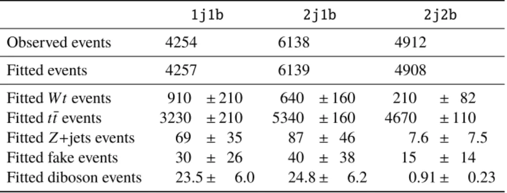
The expected and fitted yields from data are measured in the three fit regions, and the total W t signal contribution is extracted using the fitted signal strength. Table 4 shows the fitted yields of each process.

From the fitted W t yield, a cross-section is then extracted. The result is a measured cross-section of σ _{W t} = 94 ± 10 ( stat .) ₋ ⁺²⁸

23 ( syst .) pb, corresponding to an observed (expected) significance of 4 . 5 σ (3 . 9 σ ).

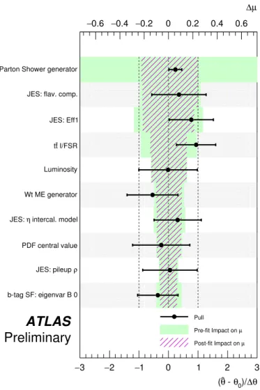
Fig. 5 shows the fit parameters with the highest post-fit impact on the signal strength, and also gives the

pre-fit impacts as well as pulls. In this plot one observes that the parameters with the highest impact are

jet energy scale uncertainties as well as the modelling uncertainties due to parton shower and t¯ t initial-

and final-state radiation. Some parameters fit to values which are significantly different from the nominal

value; t¯ t initial- and final-state radiation and effective JES component 1 each exhibit such pulls far from

nominal. Certain parameters are assigned post-fit uncertainties significantly smaller than the nominal

pre-fit uncertainty values and are thus profiled or constrained by the observed data. The most constrained

parameter here is the parton shower generator. Without profiling constraints, this uncertainty would be

among the dominant systematics, with pre-fit impacts exceeding 60% of the signal strength. However information from the 2j2b region on the t¯ t normalisation and the relative yields in the signal regions significantly constrain these uncertainties. Another feature observed in this plot is the large impacts relative to the final observed uncertainties. This comes about due to the way that each fit parameter is fixed and investigated in isolation, in the final fit correlations between parameters come into play, most significantly the floating t t ¯ normalisation. With these effects taken into account, the final uncertainties in the fit are constrained compared to the individual impacts.

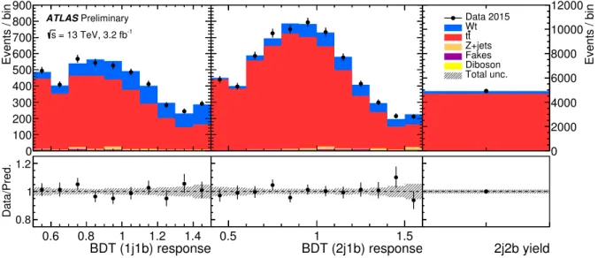
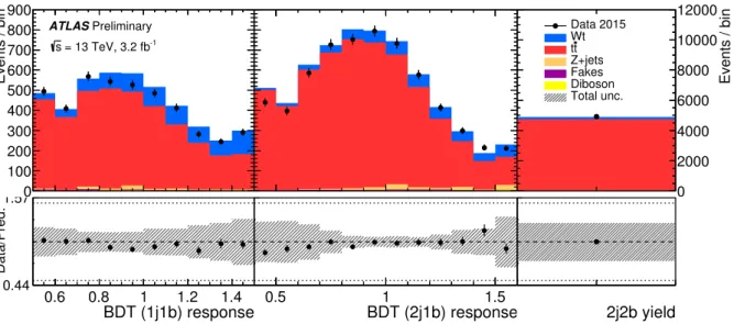
The MC predictions for the BDT response after setting all fit parameters to their final best-fit values are shown in Fig. 6, compared with the data yields. The theoretical NLO+NNLL cross-section prediction agrees well within the errors of the measured value. The t¯ t normalisation parameter, µ _{t t ¯} , is fitted to 0 . 98 ± 0 . 05, indicating that the fit does not pull the t t ¯ normalisation far from the expectation of the SM cross-section prediction.

Table 4: Fit results for an integrated luminosity of 3 . 2 fb

. The errors shown are the final fitted uncertainties on the yields, including uncertainties on signal strength, normalisation, systematic, and statistical uncertainties, taking into account correlations and constraints induced by the fit.

1j1b 2j1b 2j2b

Observed events 4254 6138 4912

Fitted events 4257 6139 4908

Fitted W t events 910 ± 210 640 ± 160 210 ± 82

Fitted t¯ t events 3230 ± 210 5340 ± 160 4670 ± 110

Fitted Z +jets events 69 ± 35 87 ± 46 7.6 ± 7.5

Fitted fake events 30 ± 26 40 ± 38 15 ± 14

Fitted diboson events 23.5 ± 6.0 24.8 ± 6.2 0.91 ± 0.23

3

− − 2 − 1 0 1 2 3

b-tag SF: eigenvar B 0 JES: pileup ρ PDF central value

intercal. model JES: η

Wt ME generator Luminosity I/FSR t t JES: Eff1 JES: flav. comp.

Parton Shower generator

µ

∆

− 0.6 − 0.4 − 0.2 0 0.2 0.4 0.6

θ )/ ∆ θ

θ - ( 3

− − 2 − 1 0 1 2 3

Pull Pre-fit Impact on µ

µ Post-fit Impact on

ATLAS Preliminary

Figure 5: List of fit parameters ranked by post-fit impact on the signal strength. Impact is calculated by fixing the

parameter to its ± 1 σ values, fixing all other parameters to their nominal values, re-fitting the signal strength, and

evaluating the change in signal strength with respect to the nominal fit. Green bands indicate the impacts computed

with σ corresponding to the pre-fit uncertainty, and hatched purple bands indicate the impacts computed with σ

corresponding to the post-fit uncertainty. The black points represent ( θ ˆ − θ

)/∆θ , the pull of the post-fit parameter

value, while the error bars are the post-fit errors on the fit parameter. The meanings of the labels and abbreviations

are detailed in Sect. 7.

Events / bin

0 100 200 300 400 500 600 700 800 900

ATLASPreliminary = 13 TeV, 3.2 fb-1

s

BDT (1j1b) response 0.6 0.8 1 1.2 1.4

Data/Pred.

0.8 1

1.2 100 200 300 400 500 600 700 800 900 0

BDT (2j1b) response

0.5 1 1.5

0.8 1

1.2 0

2000 4000 6000 8000 10000 12000

Data 2015 Wt

t t Z+jets Fakes Diboson Total unc.

Events / bin

0 2000 4000 6000 8000 10000 12000

2j2b yield 0.8

1 1.2

Figure 6: Post-fit distributions of the signal and control regions 1j1b , 2j1b , and 2j2b . The error bands represent the total uncertainties on the fitted results. The upper panels give the yields in number of events per bin, while the lower panels give the ratios of the numbers of observed events to the total prediction in each bin.

10 Conclusion

The inclusive cross-section for the associated production of a W boson and top quark is measured using 3 . 2 fb ^{− 1} of pp collision data collected at

√ s = 13 TeV by the ATLAS detector at the LHC. The analysis uses dilepton events with at least one b -tagged jet, requiring at least one isolated, central lepton with p _T > 25 GeV. Events are separated into signal and control regions based on the number of jets and b -tagged jets, then the W t signal is separated from the t¯ t background using a BDT discriminant. The cross-section is extracted by fitting templates to the data distribution, and is measured to be σ _{W t} = 94 ± 10 ( stat .) ₋ ⁺²⁸

23 ( syst .) pb. The data observation is in good agreement with the SM prediction of σ _theory = 71 . 7 ± 1 . 8 ( scale ) ± 3 . 4 ( PDF ) pb.

References

[1] N. Cabibbo, Unitary Symmetry and Leptonic Decays , Phys. Rev. Lett. 10 (12 1963) 531.

[2] M. Kobayashi and T. Maskawa, CP-Violation in the Renormalizable Theory of Weak Interaction , Progress of Theoretical Physics 49 (1973) 652.

[3] G. L. Kane, G. A. Ladinsky and C. P. Yuan, Using the top quark for testing standard-model polarization and CP predictions , Phys. Rev. D 45 (1 1992) 124.

[4] D0 Collaboration, Combination of searches for anomalous top quark couplings with 5.4 fb ^{− 1} of p p ¯ collisions , Phys. Lett. B 713 (2012) 165, arXiv: 1204.2332 [hep-ex] .

[5] J. Alwall et al., Is V( _{t b} ) ' 1? , Eur. Phys. J. C 49 (2007) 791, arXiv: hep-ph/0607115 [hep-ph] . [6] T. M. P. Tait and C. P. Yuan, Single top quark production as a window to physics beyond the

standard model , Phys. Rev. D 63 (2000) 014018, arXiv: hep-ph/0007298 .

[7] Q.-H. Cao, J. Wudka and C. P. Yuan, Search for new physics via single top production at the LHC , Phys. Lett. B 658 (2007) 50, arXiv: 0704.2809 [hep-ph] .

[8] N. Kidonakis, Theoretical results for electroweak-boson and single-top production , (2015), arXiv:

1506.04072 [hep-ph] .

[9] A. D. Martin et al., Parton distributions for the LHC , Eur. Phys. J. C 63 (2009) 189, arXiv:

0901.0002 [hep-ph] .

[10] ATLAS Collaboration, Evidence for the associated production of a W boson and a top quark in ATLAS at √

s = 7 TeV , Phys. Lett. B 716 (2012) 142, arXiv: 1205.5764 [hep-ex] .

[11] CMS Collaboration, Evidence for associated production of a single top quark and W boson in pp collisions at √

s = 7 TeV , Phys. Rev. Lett. 110 (2013) 022003, arXiv: 1209.3489 [hep-ex] . [12] CMS Collaboration, Observation of the associated production of a single top quark and a W boson

in pp collisions at √

s = 8 TeV , Phys. Rev. Lett. 112 (2014) 231802, arXiv: 1401.2942 [hep-ex] . [13] ATLAS Collaboration, Measurement of the production cross-section of a single top quark in association with a W boson at 8 TeV with the ATLAS experiment , JHEP 01 (2016) 064, arXiv:

1510.03752 [hep-ex] .

[14] ATLAS Collaboration, The ATLAS Experiment at the CERN Large Hadron Collider , JINST 3 (2008) S08003.

[15] ATLAS Collaboration, Early Inner Detector Tracking Performance in the 2015 Data at √ s = 13 TeV , ATL-PHYS-PUB-2015-051, 2015, url: http://cdsweb.cern.ch/record/2110140 . [16] ATLAS Collaboration, The ATLAS Simulation Infrastructure , Eur. Phys. J. C 70 (2010) 823, arXiv:

1005.4568 [hep-ex] .

[17] S. Agostinelli et al., GEANT4: A Simulation toolkit , Nucl. Instrum. Meth. A 506 (2003) 250.

[18] ATLAS Collaboration, The simulation principle and performance of the ATLAS fast calorimeter simulation FastCaloSim , ATL-PHYS-PUB-2010-013, 2010, url: http : / / cds . cern . ch / record/1300517 .

[19] T. Sjostrand, S. Mrenna and P. Z. Skands, A Brief Introduction to PYTHIA 8.1 , Comput. Phys.

Commun. 178 (2008) 852, arXiv: 0710.3820 [hep-ph] .

[20] ATLAS Collaboration, Summary of ATLAS Pythia 8 tunes , ATL-PHYS-PUB-2012-003, 2012, url: http://cds.cern.ch/record/1474107 .

[21] ATLAS Collaboration, Simulation of top-quark production for the ATLAS experiment at √ s = 13 TeV , ATL-PHYS-PUB-2016-004, 2016, url: http://cdsweb.cern.ch/record/2120417 . [22] P. Nason, A New method for combining NLO QCD with shower Monte Carlo algorithms , JHEP

0411 (2004) 040, arXiv: hep-ph/0409146 [hep-ph] .

[23] S. Frixione, P. Nason and C. Oleari, Matching NLO QCD computations with Parton Shower simulations: the POWHEG method , JHEP 0711 (2007) 070, arXiv: 0709.2092 [hep-ph] . [24] S. Alioli et al., A general framework for implementing NLO calculations in shower Monte Carlo

programs: the POWHEG BOX , JHEP 1006 (2010) 043, arXiv: 1002.2581 [hep-ph] .

[25] E. Re, Single-top Wt-channel production matched with parton showers using the POWHEG method , Eur. Phys. J. C 71 (2011) 1547, arXiv: 1009.2450 [hep-ph] .

[26] J. M. Campbell et al., Top-pair production and decay at NLO matched with parton showers , JHEP

04 (2015) 114, arXiv: 1412.1828 [hep-ph] .

[27] H.-L. Lai et al., New parton distributions for collider physics , Phys. Rev. D 82 (7 2010) 074024, arXiv: 1007.2241 [hep-ph] .

[28] T. Sjostrand, S. Mrenna and P. Z. Skands, PYTHIA 6.4 Physics and Manual , JHEP 05 (2006) 026, arXiv: hep-ph/0603175 [hep-ph] .

[29] J. Pumplin et al., New generation of parton distributions with uncertainties from global QCD analysis , JHEP 07 (2002) 012, arXiv: hep-ph/0201195 .

[30] P. Z. Skands, Tuning Monte Carlo Generators: The Perugia Tunes , Phys. Rev. D 82 (2010) 074018, arXiv: 1005.3457 [hep-ph] .

[31] D. J. Lange, The EvtGen particle decay simulation package , Nucl. Instrum. Meth. A 462 (2001) 152.

[32] S. Frixione et al., Single-top hadroproduction in association with a W boson , JHEP 2008 (2008) 029, arXiv: 0805.3067 [hep-ph] .

[33] J. Alwall et al., The automated computation of tree-level and next-to-leading order differential cross sections, and their matching to parton shower simulations , JHEP 1407 (2014) 079, arXiv:

1405.0301 [hep-ph] .

[34] G. Corcella et al., HERWIG 6: An Event generator for hadron emission reactions with interfering gluons (including supersymmetric processes) , JHEP 0101 (2001) 010, arXiv: hep-ph/0011363 [hep-ph] .

[35] ATLAS Collaboration, ATLAS Run 1 Pythia8 tunes , ATL-PHYS-PUB-2014-021, 2014, url:

https://cds.cern.ch/record/1966419 .

[36] ATLAS Collaboration, Monte Carlo Generators for the Production of a W or Z /γ ^∗ Boson in Association with Jets at ATLAS in Run 2 , ATL-PHYS-PUB-2016-003, 2016, url: http : //cdsweb.cern.ch/record/2120133 .

[37] T. Gleisberg et al., Event generation with SHERPA 1.1 , JHEP 2009 (2009) 007, arXiv: 0811.4622 [hep-ph] .

[38] T. Gleisberg and S. Höche, Comix, a new matrix element generator , JHEP 0812 (2008) 039, arXiv:

0808.3674 [hep-ph] .

[39] F. Cascioli, P. Maierhofer and S. Pozzorini, Scattering Amplitudes with Open Loops , Phys. Rev.

Lett. 108 (2012) 111601, arXiv: 1111.5206 [hep-ph] .

[40] S. Schumann and F. Krauss, A Parton shower algorithm based on Catani-Seymour dipole factor- isation , JHEP 0803 (2008) 038, arXiv: 0709.1027 [hep-ph] .

[41] S. Höche et al., QCD matrix elements + parton showers: The NLO case , JHEP 04 (2013) 027, arXiv: 1207.5030 [hep-ph] .

[42] ATLAS Collaboration, Multi-boson simulation for 13 TeV ATLAS analyses , ATL-PHYS-PUB- 2016-002, 2016, url: http://cdsweb.cern.ch/record/2119986 .

[43] ATLAS Collaboration, Measurement of the Z/γ boson transverse momentum distribution in pp collisions at √

s = 7 TeV with the ATLAS detector , JHEP 2014 (2014) 55, arXiv: 1406 . 3660 [hep-ex] .

[44] ATLAS Collaboration, Electron efficiency measurements with the ATLAS detector using the 2015 LHC proton-proton collision data , ATLAS-CONF-2016-024, 2016, url: https://cds.cern.

ch/record/2157687 .

[45] ATLAS Collaboration, Jet Calibration and Systematic Uncertainties for Jets Reconstructed in the ATLAS Detector at √

s = 13 TeV , ATL-PHYS-PUB-2015-015, 2015, url: https://cds.cern.

ch/record/2037613 .

[46] ATLAS Collaboration, Muon reconstruction performance of the ATLAS detector in proton–proton collision data at √

s=13 TeV , Eur. Phys. J. C 76 (2016) 292. 45 p, url: https://cds.cern.ch/

record/2139897 .

[47] M. Cacciari, G. P. Salam and G. Soyez, The Anti-k _t jet clustering algorithm , JHEP 0804 (2008) 063, arXiv: 0802.1189 [hep-ph] .

[48] M. Cacciari and G. P. Salam, Dispelling the N ³ myth for the k _t jet-finder , Phys. Lett. B 641 (2006) 57, arXiv: hep-ph/0512210 [hep-ph] .

[49] ATLAS Collaboration, Tagging and suppression of pileup jets with the ATLAS detector , ATLAS- CONF-2014-018, 2014, url: http://cdsweb.cern.ch/record/1700870 .

[50] ATLAS Collaboration, Performance of b-Jet Identification in the ATLAS Experiment , JINST 11 (2016) P04008, arXiv: 1512.01094 [hep-ex] .

[51] ATLAS Collaboration, Expected performance of the ATLAS b-tagging algorithms in Run-2 , ATL- PHYS-PUB-2015-022, 2015, url: http://cdsweb.cern.ch/record/2037697 .

[52] ATLAS Collaboration, Commissioning of the ATLAS b-tagging algorithms using t¯ t events in early Run 2 data , ATL-PHYS-PUB-2015-039, 2015, url: http : / / cdsweb . cern . ch / record / 2047871 .

[53] ATLAS Collaboration, Expected performance of missing transverse momentum reconstruction for the ATLAS detector at √

s = 13 TeV , ATL-PHYS-PUB-2015-023, 2015, url: http://cdsweb.

cern.ch/record/2037700 .

[54] ATLAS Collaboration, Performance of missing transverse momentum reconstruction with the ATLAS detector in the first proton–proton collisions at √

s = 13 TeV , ATL-PHYS-PUB-2015-027, 2015, url: http://cdsweb.cern.ch/record/2037904 .

[55] J. H. Friedman, Stochastic gradient boosting , Comput. Stat. & Data Analysis 38 (2002) 367 . [56] R. Schapire, The strength of weak learnability , Machine Learning 5 (1990) 197.

[57] A. Hocker et al., TMVA - Toolkit for Multivariate Data Analysis , PoS ACAT (2007) 040, arXiv:

physics/0703039 .

[58] F. J. Massey, The Kolmogorov-Smirnov Test for Goodness of Fit , J. Am. Stat. Assoc. 46 (1951) 68.

[59] ATLAS Collaboration, Improved luminosity determination in pp collisions at √

s = 7 TeV using the ATLAS detector at the LHC , Eur. Phys. J. C 73 (2013) 2518, arXiv: 1302.4393 [hep-ex] . [60] J. Butterworth et al., PDF4LHC recommendations for LHC Run II , J. Phys. G 43 (2016) 023001,

arXiv: 1510.03865 [hep-ph] .

[61] M. Baak et al., HistFitter software framework for statistical data analysis , Eur. Phys. J. C 75 (2015) 153, arXiv: 1410.1280 [hep-ex] .

[62] K. Cranmer et al., HistFactory: A tool for creating statistical models for use with RooFit and

RooStats , 2012, url: https://cds.cern.ch/record/1456844 .

Appendix

Events / bin

0 100 200 300 400 500 600 700 800 900

ATLASPreliminary = 13 TeV, 3.2 fb-1

s

BDT (1j1b) response 0.6 0.8 1 1.2 1.4

Data/Pred.

0.44

1.57 100 200 300 400 500 600 700 800 900 0

BDT (2j1b) response

0.5 1 1.5

0.44

1.57 0

2000 4000 6000 8000 10000 12000

Data 2015 Wt

t t Z+jets Fakes Diboson Total unc.

Events / bin

0 2000 4000 6000 8000 10000 12000

2j2b yield 0.44

1.57

Figure 7: Pre-fit distributions of the signal and control regions 1j1b , 2j1b , and 2j2b . The error bands represent

the total uncertainties on the predictions. The upper panels give the yields in number of events per bin, while the

lower panels give the ratios of the numbers of observed events to the total prediction in each bin.

Events / 20 GeV

100 200 300 400 500 600 700 800

900

Wt t t Z+jets Others Total syst.

ATLAS Preliminary = 13 TeV, 3.2 fb

s

[GeV]

E

Σ

100 150 200 250 300 350 400 450 500 Data/Pred. 0.6 0.8 1 1.2 1.4

Events / 12 GeV

100 200 300 400 500 600 700 800

900

Wt t t Z+jets Others Total syst.

ATLAS Preliminary = 13 TeV, 3.2 fb

s

) [GeV]

miss

, E

l

l

(

∆ p

− 100 − 50 0 50 100

Data/Pred. 0.6 0.8 1 1.2 1.4

Events / 8 GeV

100 200 300 400 500 600 700 800

900

Wt t t Z+jets Others Total syst.

ATLAS Preliminary = 13 TeV, 3.2 fb

s

) [GeV]

j

E

l

( p

0 20 40 60 80 100 120 140 Data/Pred. 0.6 0.8 1 1.2 1.4

Events / 0.04

100 200 300 400 500

600

Wt t t Z+jets Others Total syst.

ATLAS Preliminary = 13 TeV, 3.2 fb

s

2

)

1

l l C(

0.3 0.4 0.5 0.6 0.7 0.8 0.9 1 Data/Pred. 0.6 0.8 1 1.2 1.4

Events / 15 GeV

200 400 600 800

1000

Wt t t Z+jets Others Total syst.

ATLAS Preliminary = 13 TeV, 3.2 fb

s

) [GeV]

miss

, E

l

(

∆ p

− 150 − 100 − 50 0 50 100 150 Data/Pred. 0.6 0.8 1 1.2 1.4

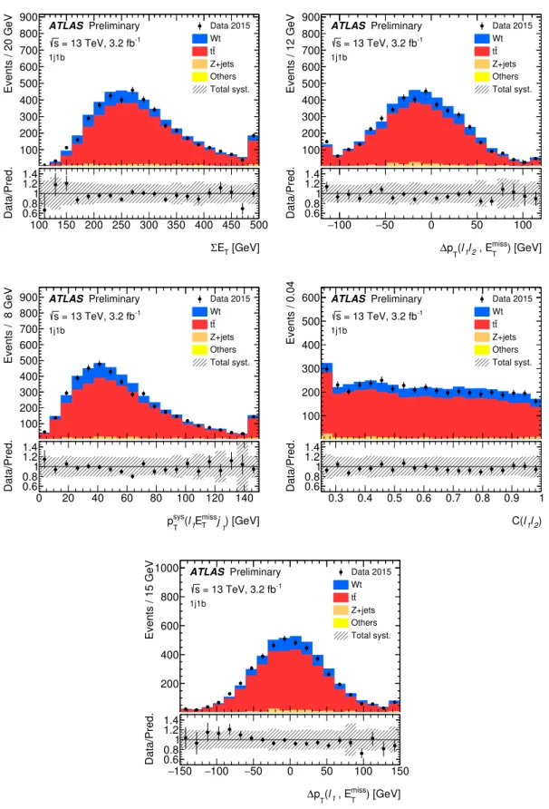
Figure 8: Distributions of the 3

to 7

most powerful BDT input variables in the 1j1b region. The signal and background are normalised to their expectation. The first and last bins of each distribution contain overflow events.

The upper panels give the yields in number of events per bin, while the lower panels give the ratios of the numbers

Events / 0.2

200 400 600 800 1000 1200

1400

Wt t t Z+jets Others Total syst.

ATLAS Preliminary = 13 TeV, 3.2 fb

s

2

)

1

j , j l

l

∆ R(

0.5 1 1.5 2 2.5 3 3.5 4 4.5

Data/Pred. 0.6 0.8 1 1.2 1.4

Events / 15 GeV

200 400 600 800 1000 1200 1400

1600

Wt t t Z+jets Others Total syst.

ATLAS Preliminary = 13 TeV, 3.2 fb

s

) [GeV]

j

l

m(

50 100 150 200 250 300

Data/Pred. 0.6 0.8 1 1.2 1.4

Events / 12 GeV

200 400 600 800 1000

1200

Wt t t Z+jets Others Total syst.

ATLAS Preliminary = 13 TeV, 3.2 fb

s

) [GeV]

miss

, E

l

l

(

∆ p

− 100 − 50 0 50 100

Data/Pred. 0.6 0.8 1 1.2 1.4

Events / 12 GeV

200 400 600 800 1000

1200

Wt t t Z+jets Others Total syst.

ATLAS Preliminary = 13 TeV, 3.2 fb

s

) [GeV]

j

, ( l P

∆

− 100 − 50 0 50 100

Data/Pred. 0.6 0.8 1 1.2 1.4

Events / 20 GeV

200 400 600 800 1000 1200 1400 1600

1800

Wt t t Z+jets Others Total syst.

ATLAS Preliminary = 13 TeV, 3.2 fb

s

) [GeV]

j

l

m(

50 100 150 200 250 300 350 400 450 Data/Pred. 0.6 0.8 1 1.2 1.4

Events / 9 GeV

200 400 600 800 1000 1200 1400

Data 2015 Wt

t t Z+jets Others Total syst.

ATLAS Preliminary = 13 TeV, 3.2 fb

s

) [GeV]

l

( p

20 40 60 80 100 120 140 160 180 200 Data/Pred. 0.6 0.8 1 1.2 1.4

Figure 9: Distributions of the 3

to 8

most powerful BDT input variables in the 2j1b region. The signal and

background are normalised to their expectation. The first and last bins of each distribution contain overflow events.

Events / 0.35 GeV

200 400 600 800 1000 1200 1400

1600

Wt t t Z+jets Others Total syst.

ATLAS Preliminary = 13 TeV, 3.2 fb

s

) [GeV]

j

E

l

l

)(

(p

σ

0 1 2 3 4 5 6 7

Data/Pred. 0.6 0.8 1 1.2 1.4

Events / 0.2

200 400 600 800 1000 1200

1400

Wt t t Z+jets Others Total syst.

ATLAS Preliminary = 13 TeV, 3.2 fb

s

1

) , j l

∆ R(

0.5 1 1.5 2 2.5 3 3.5 4 4.5

Data/Pred. 0.6 0.8 1 1.2 1.4

Events / 4 GeV

200 400 600 800 1000 1200 1400 1600

1800

Wt t t Z+jets Others Total syst.

ATLAS Preliminary = 13 TeV, 3.2 fb

s

) [GeV]

j

( p

20 30 40 50 60 70 80 90 100 Data/Pred. 0.6 0.8 1 1.2 1.4

Events / 0.2 GeV

200 400 600 800 1000 1200 1400

1600

Wt t t Z+jets Others Total syst.

ATLAS Preliminary = 13 TeV, 3.2 fb

s

) [GeV]

j

j

E

l

l

)(

(p

σ

0 0.5 1 1.5 2 2.5 3 3.5 4

Data/Pred. 0.6 0.8 1 1.2 1.4

Events / 30 GeV

200 400 600 800 1000 1200 1400 1600 1800

2000

Wt t t Z+jets Others Total syst.

ATLAS Preliminary = 13 TeV, 3.2 fb

s

) [GeV]

j

j

l

m(

0 100 200 300 400 500 600

Data/Pred. 0.6 0.8 1 1.2 1.4

Events / 15 GeV

200 400 600 800 1000 1200 1400 1600

1800

Wt t t Z+jets Others Total syst.

ATLAS Preliminary = 13 TeV, 3.2 fb

s

) [GeV]

j

l

m(

50 100 150 200 250 300

Data/Pred. 0.6 0.8 1 1.2 1.4

Figure 10: Distributions of the 9

to 14

most powerful BDT input variables in the 2j1b region. The signal and background are normalised to their expectation. The first and last bins of each distribution contain overflow events.

The upper panels give the yields in number of events per bin, while the lower panels give the ratios of the numbers