Search for Dark Matter produced in association with a Standard Model Higgs boson decaying to b-quarks using the full Run 2 collision data with the

ATLAS-CONF-2021-006 26March2021

ATLAS CONF Note

ATLAS-CONF-2021-006

24th March 2021

Search for Dark Matter produced in association with a Standard Model Higgs boson decaying to b-quarks using the full Run 2 collision data with the

ATLAS detector

The ATLAS Collaboration

The production of Dark Matter in association with Higgs bosons is predicted in several extensions of the Standard Model. An exploration of such scenarios is presented, considering final states with missing transverse momentum and b -tagged jets consistent with a Higgs boson.

The analysis uses proton-proton collision data at a centre-of-mass energy of 13 TeV recorded by the ATLAS experiment at the LHC during Run 2, amounting to an integrated luminosity of 139 fb

. The analysis, when compared to previous searches, benefits from an increased dataset, but also has further improvements providing sensitivity to a wider spectrum of signal scenarios. These improvements include both an optimised event selection and advances in the object identification, such as the use of the likelihood-based significance of the missing transverse momentum and variable-radius track jets. No significant deviation from Standard Model expectations is observed. The results are interpreted in two benchmark models with two Higgs doublets extended by either a heavy vector boson Z

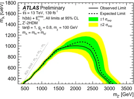
or a pseudoscalar singlet a and which provide a Dark Matter candidate χ . In the case of the Two-Higgs-Doublet model with an additional vector boson Z

, the observed limits extend up to a Z

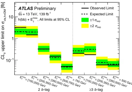
mass of 3.1 TeV at 95% confidence level for a mass of 100 GeV for the Dark Matter candidate. For the Two-Higgs-Doublet model with an additional pseudoscalar a , masses of a are excluded up to 520 GeV and 240 GeV for a Dark Matter mass of 10 GeV and, respectively, tan β = 1 and tan β = 10. Limits on the visible cross sections are set and range from to 0.05 fb to 3.26 fb, depending on the missing transverse momentum and b -quark jet multiplicity requirements.

© 2021 CERN for the benefit of the ATLAS Collaboration.

Reproduction of this article or parts of it is allowed as specified in the CC-BY-4.0 license.

1 Introduction

Various astrophysical observations based on gravitational interactions [1, 2] strongly support the existence of Dark Matter (DM) which interacts through neither the strong nor the electromagnetic force. However, the Standard Model of particle physics (SM) provides no suitable DM candidate particle. There are many complementary search strategies for DM including direct [3–7] and indirect detection experiments [8] as well as searches at particle colliders.

Since DM particles do not interact electromagnetically or strongly even direct-detection experiments have low detection efficiencies. Therefore, instead of attempting to detect them directly, any DM particles produced in proton-proton collisions at the Large Hadron Collider [9] (LHC) would be deduced from an imbalance in the transverse momentum measured in that collision event ( E

T

). This means that DM particles can only be detected if they are produced in association with visible particles. When there is only one such particle this gives rise to event topologies referred to as ‘mono- X ’ final states, where X refers to the visible particle. Prominent examples of these topologies are the mono-jet [10–12], mono- Z /W [13–15]

and mono-photon [16–18] final states.

Mono- X topologies are typically dominated by cases where the visible particle is produced from initial state radiation (ISR), as the couplings between the SM particle X and the initial state quarks or gluons are much larger than its couplings with the final state DM particles. A counter example is the case where the visible particle is a SM Higgs boson (named the mono-Higgs signature). Given that the coupling of the Higgs boson to light quarks and gluons is highly suppressed a Higgs boson is more likely to be produced through final state radiation (FSR) or as part of the same process that produces the DM particles.

This means that this topology is only sensitive to models where the Higgs boson couples directly to DM or some other beyond SM (BSM) particle involved in the DM production. However, in these cases the DM-SM interaction is directly probed [19], potentially providing more information about the structure of the DM-SM coupling in the event of a discovery. There are also many models where the coupling between BSM particles and the Higgs boson is enhanced, for instance models where DM is connected to electroweak symmetry breaking [20, 21] or where DM particles couple to the SM only through the Higgs sector (Higgs portal models) [22]. These features make the mono-Higgs signature an important part of the LHC DM search programme.

The Two-Higgs-Doublet model (2HDM) [23] extends the SM with a second Higgs doublet. This predicts a total of five Higgs bosons after mixing: two charged scalars H

, two neutral CP-even scalars h and H as well as one neutral CP-odd scalar A . Two simplified benchmark signal models are used: the Z

-2HDM [24]

and 2HDM+ a [25, 26]. In all models considered here the mass of the lighter neutral CP-even scalar h is required to match that of the SM Higgs boson.

The Z

-2HDM adds an additional heavy vector boson, denoted Z

, whose coupling to quarks g

and mass m

are free parameters. The production mechanism for the mono-Higgs signature is shown in Figure 1.

DM is introduced into the model as a new fermion which couples only to the down-type Higgs doublet. Its coupling to the CP-odd scalar A , denoted g

, and mass m

are also free parameters. This model is used mainly as a benchmark for high-mass resonances.

The 2HDM+ a scenario is the simplest renormalisable and gauge-invariant extension of a simplified

pseudoscalar mediator model. It adds a new pseudoscalar singlet which mediates the interactions between

the SM and a singlet fermion χ identified as the DM candidate. The coupling between the pseudoscalar

and DM singlets, denoted y

, and the mass of the DM m

are free parameters. This singlet mixes with

the pseudoscalar A from the two Higgs doublets, with the mixing angle θ and the mass of the resulting

q h Z’

A q

Figure 1: Feynman diagram for the production of the mono-Higgs signature in theZ⁰-2HDM.

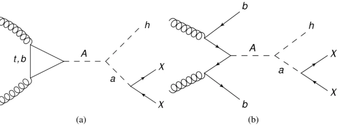
pseudoscalar a being free parameters of the model. A major advantage of the 2HDM+ a scenario over more simplified models is that it generates a wider variety of experimental signatures which can provide complementary exclusion from different types of experiment. There are two main production mechanisms for the mono-Higgs signature in this model, as shown in Figure 2.

t , b A

a

h

(a)

b

b A

a h

(b)

Figure 2: Feynman diagrams for the main production mechanisms of the mono-Higgs signature in the 2HDM+a scenario: gluon-gluon fusion(a)andb-associated production(b).

In the type-II 2HDM considered in this paper the coupling between down-type quarks and the A boson scales with tan β , the ratio of the vacuum expectation values of the two Higgs doublets. This means that for low tan β values (tan β . 5) the gluon-gluon fusion ( gg F) mechanism shown in Figure 2(a) dominates, whereas for higher tan β values the b -associated production ( bb A) shown in Figure 2(b) is dominant. Signal grids are generated where each of the two production mechanisms are used exclusively. For each grid a tan β value is chosen that ensures that the corresponding production mechanism is dominant: tan β = 1 for the ggF grid and tan β = 10 for the bbA grid.

Similar analyses were performed using data taken during the years 2015-2016 by ATLAS [27] and CMS [28]. Other mono-Higgs analyses were also performed on the same datasets in final states where the Higgs decays to a pair of photons in ATLAS [29] or either a pair of photons or a τ

τ

pair in CMS [30].

Beyond the large increase in luminosity (from 36 fb

to 139 fb

) a number of analysis improvements extend the sensitivity beyond the previous ATLAS search.

In the previous ATLAS result, events were required to have either one or two b -jets, whereas in this search

events are divided into regions with either exactly two b -jets or at least three. Removing events with one

b -jet reduces sensitivity to backgrounds from processes involving W/Z bosons and including events with

at least three b -jets improves the sensitivity to the 2HDM+ a bb A production mechanism, which was not

considered in the previous ATLAS result.

The analysis also benefits from using particle flow objects for jet reconstruction [31], neural-network based b -jet [32] and τ -lepton [33] identification and variable-radius track jets [34] to identify boosted Higgs boson candidates. In order to reduce backgrounds containing fake E

T

the likelihood-based E

T

significance S [35] is used to further improve over the previous search result. The event selections were re-optimised resulting in an improved sensitivity with fewer, more efficient selections in particular enhancing the sensitivity to highly boosted signals.

2 ATLAS detector

The ATLAS detector [36] at the LHC covers nearly the entire solid angle around the collision point.

It consists of an inner tracking detector surrounded by a thin superconducting solenoid, electromagnetic and hadronic calorimeters, and a muon spectrometer incorporating three large superconducting toroidal magnets.

The inner-detector system (ID) is immersed in a 2 T axial magnetic field and provides charged-particle tracking in the range |η| < 2 . 5.

The high-granularity silicon pixel detector covers the vertex region and typically provides four measurements per track, the first hit being normally in the insertable B-layer (IBL) installed before Run 2 [37, 38]. It is followed by the silicon microstrip tracker (SCT) which usually provides eight measurements per track.

These silicon detectors are complemented by the transition radiation tracker (TRT), which enables radially extended track reconstruction up to |η| = 2 . 0. The TRT also provides electron identification information based on the fraction of hits (typically 30 in total) above a higher energy-deposit threshold corresponding to transition radiation.

The calorimeter system covers the pseudorapidity range |η| < 4 . 9. Within the region |η| < 3 . 2, electromagnetic calorimetry is provided by barrel and endcap high-granularity lead/liquid-argon (LAr) calorimeters, with an additional thin LAr presampler covering |η| < 1 . 8, to correct for energy loss in material upstream of the calorimeters. Hadronic calorimetry is provided by the steel/scintillating-tile calorimeter, segmented into three barrel structures within |η | < 1 . 7, and two copper/LAr hadronic endcap calorimeters. The solid angle coverage is completed with forward copper/LAr and tungsten/LAr calorimeter modules optimised for electromagnetic and hadronic measurements respectively.

The muon spectrometer (MS) comprises separate trigger and high-precision tracking chambers measuring the deflection of muons in a magnetic field generated by superconducting air-core toroids. The field integral of the toroids ranges between 2.0 and 6.0 T m across most of the detector. A set of precision chambers covers the region |η | < 2 . 7 with three layers of monitored drift tubes, complemented by cathode-strip chambers in the forward region, where the background is highest. The muon trigger system covers the range |η| < 2 . 4 with resistive-plate chambers in the barrel, and thin-gap chambers in the endcap regions.

Interesting events are selected to be recorded by the first-level trigger system implemented in custom hardware, followed by selections made by algorithms implemented in software in the high-level trigger [39].

The first-level trigger reduces the output event rate from the 40 MHz bunch crossing rate to below 100 kHz, which the high-level trigger further reduces in order to record events to disk at about 1 kHz.

1ATLAS uses a right-handed coordinate system with its origin at the nominal interaction point (IP) in the centre of the detector and thez-axis along the beam pipe. Thex-axis points from the IP to the centre of the LHC ring, and they-axis points upwards.

Cylindrical coordinates(r, φ)are used in the transverse plane,φbeing the azimuthal angle around thez-axis. The pseudorapidity is defined in terms of the polar angleθasη=−ln tan(θ/2). Angular distance is measured in units of∆R≡p

(∆η)2+(∆φ)2.

3 Data and simulated event samples

This search uses 139 fb

of proton-proton collision data recorded by the ATLAS detector at a centre- of-mass energy of 13 TeV during the years 2015-2018 (Run 2). The uncertainty on the total integrated luminosity for the full Run 2 dataset is 1.7% [40]. All events used are required to pass basic data quality requirements which ensure that all components of the ATLAS detector were correctly functioning [41].

Events selected for the analysis search regions were collected by the primary E

T

triggers [42] which select those which have a large transverse momentum imbalance. The algorithms used to calculate the imbalance and the thresholds required varied throughout the dataset. The ‘primary’ E

T

trigger in a run is the most efficient available E

T

trigger, in all cases reaching full efficiency by an offline E

T

value of approximately 200 GeV.

Simulated event samples corresponding to the Z

-2HDM signal were generated at leading order (LO) in QCD in the 5-flavour scheme using MadGraph5_aMC@NLO v2.6.5 [43] interfaced to Pythia 8.240 [44]

using the A14 set of tuned parameters [45]. In these samples the coupling of the Z

boson to quarks was fixed to g

= 0 . 8, the mass of the DM candidate was set to m

= 100 GeV, the Aχ χ ¯ coupling g

was set to 1, tan β was set to 1 and the alignment limit, i.e. sin ( β − α) = 1, was assumed, where α is the mixing angle between the two CP-even Higgs bosons. The samples were generated with varying m

between 600 and 3600 GeV and m

between 300 and 1300 GeV.

Simulated event samples corresponding to the 2HDM+ a signal were generated at LO using Mad- Graph5_aMC@NLO v2.6.7 interfaced to Pythia 8.244 with the A14 set of tuned parameters. Samples were generated separately for the gg F and bb A production modes, with the former generated in the 4-flavour scheme setting tan β = 1 and the latter in the 5-flavour scheme setting tan β = 10. Following the recommendations of the LHC Dark Matter working group [25], the mass of the DM candidate was set to m

= 10 GeV, the Yukawa coupling between the DM candidate and the pseudoscalar a was set to y

= 1 and the Higgs quartic couplings were set to λ

= λ

= λ

= 3. The chosen value of m

ensures that the a → χ χ branching ratio is significant for all values of m

used. The pseudoscalar mixing angle was set to sin θ = 0 . 35 and the alignment limit was assumed. The samples were generated with varying m

between 250 and 2000 GeV and m

between 100 and 600 GeV.

For all signal samples the masses of the heavy Higgs bosons were considered degenerate ( m

= m

= m

).

The mass of the lightest CP-even Higgs boson was set to match the SM Higgs boson, i.e. m

= 125 GeV.

Background events from the production of a single weak vector boson in association with jets ( V = W, Z ) or of a pair of weak bosons (diboson) were simulated using Sherpa v2.2.1 [46] with Sherpa v2.2.2 used for gg -initiated diboson production. For the V +jets samples next-to-leading-order (NLO) matrix elements for up to two jets and LO matrix elements for up to four jets were calculated using the Comix [47] and OpenLoops [48, 49] libraries. For the q q ¯ -initiated diboson samples NLO matrix elements for up to one additional jet and LO matrix elements for up to three additional jets were used while the gg -initiated processes were generated using LO matrix elements for up to one additional jet. The samples were matched with the Sherpa parton shower [50] using the MEPS@NLO prescription [51–54].

Samples corresponding to the top-quark pair ( t¯ t ), single top-quark ( s , t and Wt channels) and t t h ¯ processes

were generated using PowhegBox v2 [55–62] with h

set to 1 . 5 m

and m

= 172 . 5 GeV. The h

parameter regulates the transverse momentum ( p

) of the high- p

emission against which the t¯ t system

recoils. The inclusive cross-section for these processes were corrected to the next-to-next-to-leading-

order (NNLO)+next-to-next-to-leading logarithmic (NNLL) prediction [63–69] for t¯ t , NLO+NNLL for

Wt [70, 71], NLO for s and t -channel single top-quark production [70, 71] and NLO QCD+electroweak (EW)

for t t h ¯ [72]. The diagram removal scheme [73] was used in the Wt samples to avoid double counting contributions from t t ¯ processes.

The W / Z + h samples were generated using PowhegBox v2. The cross-sections of the q q ¯ -initiated processes were calculated at NNLO and NLO in QCD and EW respectively, using the Powheg MiNLO procedure [74, 75]. The cross-sections of the gg -initiated processes were calculated at NLO+next-to-leading logarithmic (NLL) in QCD [76–78].

The t tV ¯ samples were generated using MadGraph5_aMC@NLO v2.3.3 at NLO. The cross-sections were calculated at NLO QCD and EW accuracies as provided by Ref. [72].

All samples were generated using the NNPDF3.0nlo parton distribution function (PDF) set [79] apart from the Sherpa W / Z +jets and diboson samples which were generated using the NNPDF3.0nnlo PDF set along with a dedicated tune developed by the Sherpa authors and the t -channel single top-quark production samples which were generated using the NNPDF3.0nlonf4 PDF set. The PowhegBox samples were interfaced with Pythia 8.230 for the parton shower and hadronisation. Of these, the t t ¯ , single top-quark and t¯ t h samples used the NNPDF2.3lo PDF set [79] and the A14 tune [80] while the W / Z + h samples used the CTEQ6L1 PDF set [81] and the AZNLO tune [82]. For the PowhegBox top-quark processes the decays of b - and c -hadrons were simulated using EvtGen v1.6.0 [83]. The t¯ tV samples were interfaced with Pythia 8.210 using the same tune and PDF set as the PowhegBox t t ¯ , single top-quark and t¯ t h processes, using EvtGen v1.2.0 for the decays of b - and c -hadrons.

In order to simulate the effect of additional pp collisions in the same and neighbouring bunch crossings (pile-up) all samples were overlaid with multiple pp collisions simulated with Pythia 8.186 using the NNPDF2.3lo PDF set and the A3 tune [84]. The response of the detector was modelled with a detector simulation [85] based on Geant4 [86].

4 Object definitions

Primary Vertex

Primary vertices are constructed using at least two ID tracks with p

> 500 MeV [87]. The primary vertex with the largest sum of squared track transverse momenta ( Í

p

T

) is selected as the hard-scatter vertex, henceforth only referred to as the primary vertex.

Jets

Jets are reconstructed using the anti- k

algorithm [88, 89]. The analysis considers three types of jets to better suit different event topologies. Small-radius (small- R ) jets are constructed from particle-flow objects formed from ID tracks and calorimeter clusters [31] using a radius parameter of R = 0 . 4. This radius parameter is designed to capture the jet initiated by a gluon, light quark or b quark. Small- R jets are classified as central ( |η| < 2 . 5) or forward (2 . 5 < |η| < 4 . 5). Central small- R jets are required to have p

> 20 GeV and forward small- R jets p

> 30 GeV. In order to remove the impact of jets predominantly formed from particles from pile-up vertices, central small- R jets are required to pass the ‘Tight’ Jet Vertex Tagger [90] (JVT) working point (WP)

.

2The JVT selection is applied on jets with 20<p_T <60 GeV and|η|<2.4.

In topologies where the Higgs boson decay cannot be resolved into two small-radius jets, large-radius (large- R ) jets with a radius parameter of R = 1 . 0 are used, constructed from calorimeter clusters calibrated using the local hadronic cell weighting (LCW) scheme [91]. This radius parameter is designed to capture jets produced from the decay of boosted heavier objects, such as Higgs bosons. To reduce the impact of pile-up, these jets are then ‘trimmed’, removing any R = 0 . 2 subjets which have less than 5% of the original jet energy [92]. In order to identify subjets originating from b -hadrons within the large- R jets, jets are also constructed from ID tracks, using a variant of the anti- k

algorithm with a radius parameter that shrinks as the p

of the proto-jet increases [34]. These are referred to as variable-radius (variable- R ) track jets and are ghost-associated [93] to the large- R jets. The radius parameter is set to R = 30 GeV /p

, with minimum and maximum values of 0.02 and 0.4, respectively. The reduced radius at high p

allows the algorithm to reconstruct separate jets from close-by b -hdarons, such as in highly boosted h → b b ¯ decays.

Both small- and large- R jet energies are calibrated using a sequence of simulation-derived corrections.

Small- R jets additionally have an area-based subtraction applied to reduce the impact of pile-up, as well as a series of additional data-derived corrections [94].

Central small- R jets and variable- R track jets containing b -hadrons are identified using the DL1 tagger [32].

This multivariate algorithm uses information from the impact parameters of ID tracks, secondary vertices within the jets as well as the reconstructed flight paths of b - and c -hadrons within the jet. For both classes of jet a WP is chosen which tags jets containing b -hadrons with 77% efficiency in t¯ t . The decays of these b -hadrons can produce muons which are vetoed when building particle flow objects and therefore are not included in the energies of either the small- or large- R jets. In order to correct for this, the four-momenta of non-isolated muons falling inside these jet cones can be added into the jet, improving the resolution of their four-momenta. For small- R (large- R ) jets this is done for the closest (two closest) muons to the jet axis. This correction is only used when calculating the mass of the Higgs boson candidate m

and was shown in Ref. [95] to improve the resolution of this measurement. Correcting m

in this way improves the ability of the fit to separate the signal from the major backgrounds.

Leptons

Leptons are divided into ‘signal’ and ‘baseline’ categories. Events with baseline leptons are vetoed in the analysis search regions and signal leptons are used to define regions to constrain background components.

Electrons are reconstructed from a track which is coincident with a cluster of cells in the electromagnetic calorimeter [96]. They are then identified using a multivariate likelihood technique, using several features including the shape of the measured shower, the track quality and the distribution of energy within the calorimeter [97]. For this analysis, the ‘LooseAndBLayer’ WP [97] is used for both signal and baseline electrons. Isolation selections are also applied to distinguish between electrons produced in the initial collision or decays of W/Z bosons or τ -leptons (prompt) and those produced in decays of other objects [97].

Isolation requirements are made on the energy measured in calorimeter clusters and tracks around the electron. For signal electrons with p

< 200 GeV and all baseline electrons the total energy of clusters within ∆R < 0 . 2 of the electron, excluding the electron cluster, is required to be less than 20% of the p

of the electron. The total p

of tracks associated to the primary vertex within a cone whose radius is set to the smaller of R = 10 GeV /p

and 0.2, excluding the electron track, is required to be less than 15% of the p

of the electron. For signal electrons with p

> 200 GeV the total energy of clusters within ∆R < 0 . 2 of the electron is required to be less than the smaller of 0 . 015 × p

and 3 . 5 GeV. For these electrons no track-based isolation selection is applied. Both baseline and signal electrons are required to have |η | < 2 . 47.

Baseline electrons are required to have p

> 7 GeV and signal electrons p

> 27 GeV. In order to ensure

that they are compatible with the primary vertex, the track from which the electron is reconstructed is required to have σ(d

) < 5 and | z

sin θ | < 0 . 5 mm where σ(d

) is the significance of the transverse impact parameter and z

is the longitudinal impact parameter.

Muons are reconstructed by associating track segments formed in the MS with a track from the ID [98].

Identification is performed through selections on the qualities of the tracks used in the reconstruction, as well as their compatibility, for example, in the measurements of p

in the muon spectrometer and inner detector. Similarly to electrons, isolation selections are also applied. Baseline muons are required to pass the ‘Loose’ identification WP and signal muons are required to pass the ‘Medium’ identification WP [98].

For baseline muons, the total energy of clusters within ∆R < 0 . 2 of the muon is required to be less than 30% of the p

of the muon. For signal muons, additionally the total p

of tracks within ∆R < 0 . 2 of the muon’s primary track is required to be less than 1.25 GeV. Both baseline and signal muons are required to satisfy |η | < 2 . 5, σ(d

) < 3 and |z

sin θ | < 0 . 5 mm. Baseline muons are required to have p

> 7 GeV and signal muons p

> 25 GeV.

Hadronically decaying τ -lepton reconstruction is seeded from R = 0 . 4 anti- k

jets built using the LCW- calibrated clusters [99]. As hadronic τ -lepton decays yield either one or three charged pions the jets are required to have either one or three tracks within ∆R < 0 . 2 of the jet axis. A recurrent neural network (RNN) classifier is used to identify the τ -leptons [33]. The inputs to the RNN are built from the clusters and tracks associated to the τ -lepton. All τ -leptons are required to pass the ‘VeryLoose’ WP [33] and have

|η| < 2 . 5 and p

> 20 GeV. As there is no dedicated τ -lepton control region no signal τ -lepton selection is defined.

Overlap removal

In order to avoid the same detector signals being interpreted as different objects, an overlap removal procedure is applied as follows. If any object is rejected at one step it is not considered in later steps. First, if any two electrons share a track the electron with the lower p

is removed. Next, any τ -leptons within

∆R < 0 . 2 of an electron or muon are removed. Then, any electrons which share a track with a muon are removed. If any small- R jet is within ∆R < 0 . 2 of an electron it is removed, then if any electron is within a p

-dependent cone of a small- R jet it is removed. If any small- R jet with fewer than three tracks has an associated muon or is within ∆R < 0 . 2 of one it is removed, then any muons within a p

-dependent cone of a small- R jet are removed. Next, any small- R jets within ∆R < 0 . 2 of a τ -lepton are removed. Finally, any large- R jets within ∆R < 1 . 0 of an electron are removed.

Track jets do not participate in the overlap removal as they are only used for b -tagging.

Missing transverse energy

The missing transverse energy ( E

T

) [100] is the magnitude of the missing transverse momentum, defined as the negative vector sum of the transverse momenta of all the observable objects in the event in addition to a soft term including ID tracks not associated to any of the other objects. The E

T

is constructed from the baseline electrons and muons as well as all small- R jets. The E

T

reconstruction uses a separate overlap removal procedure which takes into account detector deposits from each object included [100]. In control regions a modified definition of E

T

is used in which electrons and muons are treated as invisible, E

lep, invis

.

Object mismeasurements, especially of jets, are the main source of fake E

T

. Therefore the E

T

significance ( S ) [35] is defined to assess the likelihood that the E

T

is really due to invisible particles or is more likely to come from mismeasurements. It is calculated using the expected resolutions of all objects which enter the E

T

calculation and the correlations between them.

5 Event selection

The basic target final state topology is a Higgs boson decaying into two b quarks produced with a significant imbalance in the measured transverse momentum. Events are divided into non-overlapping regions designed either to be enriched in the signal process (signal regions) or in a significant background process (control regions). Control regions differ from signal regions primarily through requiring the presence of one or two lepton(s), whereas signal regions veto events containing baseline leptons.

As the angle between the two b -jets produced in the Higgs boson decay is inversely proportional to the p

of the Higgs boson, in cases where the Higgs boson is significantly boosted it can become difficult to reconstruct the two b -quarks as separate jets. This motivates splitting the analysis into ‘resolved’ regions in which the decay products of the Higgs boson are reconstructed as two separate jets and ‘merged’ regions in which the entire Higgs boson decay is reconstructed as a single jet.

In b -associated production within the 2HDM+ a benchmark model, the Higgs boson and DM particles are produced with an extra pair of b quarks from gluon splitting. Therefore, to enhance sensitivity to these models, all regions are further split into those requiring exactly two b -jets and those requiring ≥ 3 b -jets (referred to as 2 b -tag and ≥ 3 b -tag respectively).

5.1 Common selections

Events which do not have a reconstructed primary vertex are rejected. Events are also rejected if found to contain fake jets caused by beam-induced backgrounds, cosmic ray showers and noisy calorimeter cells.

Events are required to have E

T

> 150 GeV and are vetoed if they contain a baseline τ -lepton. In order to further reduce the background from τ -lepton decays, events are also vetoed if they have any small- R jets with ∆ φ( jet , E

T

) < π/ 8 where the track multiplicity in the jet is between 1 and 4. This selection is referred to as the ‘extended τ -lepton veto’. A further source of background is E

T

arising from either heavy-flavour decays in a jet or a jet which is severely mismeasured. In these cases, the E

T

tends to be aligned with the jet, therefore events where any of the three leading small- R jets have ∆ φ( jet , E

T

) < 20°

are rejected. For control regions these requirements use E

T, lep. invis.

rather than E

T

.

Only loose selections are placed on the mass of the Higgs boson candidate ( m

) as this is then used as the

discriminating variable for the final fit. This range is 50 GeV < m

< 280 GeV for the resolved regions and

50 GeV < m

< 270 GeV for the merged regions with the lower limit chosen to be the lowest calibrated

large- R jet mass and the upper limit chosen to be significantly larger than the Higgs boson mass with the

precise value being determined by the m

binning used in the fit, as determined according to the available

statistics.

5.2 Signal regions

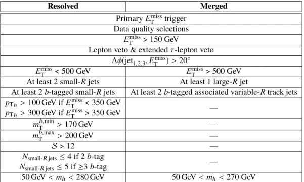
The signal region selections for both merged and resolved regions are summarised in Table 1. All signal region events are required to have passed the primary E

T

trigger [42]. In order to reduce the contribution of SM processes producing E

T

through the decay W → `ν , events are rejected if they contain any baseline electron or muon.

5.2.1 Resolved regions

The resolved regions are defined by selecting events with E

T

< 500 GeV. Events in the resolved regions are required to have at least two b -tagged small- R jets, with the two with the highest p

forming the Higgs boson candidate. The combined p

of this two-jet system ( p

) is required to be greater than 100 GeV and its mass is corrected for close-by muons as described in Section 4 to form m

.

The dominant background in the resolved region is t t ¯ production where one top quark decays leptonically, but the lepton is either not reconstructed or not correctly identified. In these cases, all the E

T

in the event (beyond that from mismeasurement) originates from the decay of one of the two W bosons, therefore the transverse mass between the E

T

and the corresponding b -jet should be approximately bounded from above by the top-quark mass, where the transverse mass is defined as

m

T

= q

2 p

T

E

T

( 1 − cos ∆φ(p

T

, E

T

)) where p

T

and p

T

are respectively defined as the p

of the b -jet which is closest to (min) or furthest from (max) the E

T

in φ . Events are required to pass m

T

> 170 GeV and m

T

> 200 GeV.

In order to suppress contributions from multijet backgrounds, the object-based E

T

significance is required to satisfy S > 12. After this selection data-driven estimates of the remaining multijet contribution to the signal regions were found to be substantially smaller than the expected statistical uncertainty of the data so the impact of multijet processes is not included in the background estimation. The signal models studied typically have fewer reconstructed jets than the dominant backgrounds. Therefore events with exactly two b -tagged jets (2 b -tag) are required to have at most four small- R jets, where only central jets are counted.

For events with at least three b -tagged jets ( ≥ 3 b -tag), this requirement is relaxed to five small- R jets to ensure sufficient statistics in the corresponding control regions.

The 2 b -tag and ≥ 3 b -tag selections are split into three E

T

bins: 150 GeV < E

T

< 200 GeV, 200 GeV < E

T

< 350 GeV and 350 GeV < E

T

< 500 GeV. In the highest E

T

bin the requirement on p

is tightened to being greater than 300 GeV. This leads to six resolved signal regions: one corresponding to each combination of E

T

bin and number of b -tagged jets.

The E

T

triggers become fully efficient at an offline E

T

value close to 200 GeV, however the analysis also uses events in the range 150 GeV < E

T

< 200 GeV. In order to correct for Monte Carlo (MC) mismodelling of the E

T

trigger response, the trigger efficiency must be measured in both data and simulation and scale factors calculated to correct the simulation. Given that the E

T

triggers use calorimeter information only, they treat muons as invisible particles, meaning that E

T

trigger efficiencies can be measured using events selected by single-muon triggers [101]. The scale factors are calculated as a function of E

T,lep,invis

in a region whose selection matches the 150 GeV < E

T

< 200 GeV and 2 b -tag region except that all E

T

selections are dropped, exactly one b -tagged jet is required and exactly one

Resolved Merged Primary E

T

trigger Data quality selections

E

T

> 150 GeV

Lepton veto & extended τ -lepton veto

∆ φ( jet

, E

T

) > 20°

E

T

< 500 GeV E

T

> 500 GeV At least 2 small- R jets At least 1 large- R jet

At least 2 b -tagged small- R jets At least 2 b -tagged associated variable- R track jets p

> 100 GeV if E

T

< 350 GeV p

> 300 GeV if E

—

T

> 350 GeV m

T

> 170 GeV —

m

T

> 200 GeV —

S > 12 —

N

≤ 4 if 2 b -tag N

≤ 5 if ≥ 3 b -tag —

50 GeV < m

< 280 GeV 50 GeV < m

< 270 GeV

Table 1: Summary of selections used to define the signal regions used in the analysis. The kinematic variables are defined in the text.

signal muon is required. Events containing electrons are still vetoed. The scale factors have values in the range 0.95–1.0.

5.2.2 Merged regions

The merged regions are defined by selecting events with E

T

> 500 GeV. At least one large- R jet is required, and the two leading variable- R track jets associated to the leading large- R jet are required to be b -tagged. This large- R jet is defined to be the Higgs boson candidate and its mass is corrected for close-by muons as described in Section 4 to form m

. Events are separated into those which have no additional b -tagged variable- R track jets (2 b -tag selection) and those which have at least one such b -tagged variable- R track jet not associated to the Higgs boson candidate ( ≥ 3 b -tag selection).

The merged 2 b -tag selection is split into two E

T

bins, 500 GeV < E

T

< 750 GeV and E

T

> 750 GeV, while no further splitting is done for ≥ 3 b -tag selection.

5.3 Background modelling and control regions

The dominant backgrounds in the signal regions consist of t t ¯ and W/Z bosons produced in association with two heavy-flavour jets arising from hadrons containing b or c quarks ( W +HF or Z +HF). In the 2 b -tag resolved regions the dominant backgrounds are t¯ t and Z +HF, with the latter becoming more important as the E

T

increases. The 2 b -tag merged regions are dominated by Z +HF. Both the resolved and merged

≥ 3 b -tag regions are dominated by t t ¯ , where the extra b -jet typically is a mis-tagged jet originating from a hadronic W boson decay. At higher E

T

values the Z +HF background becomes important again.

The t¯ t , W +HF and Z +HF contributions are modelled using simulation with their normalisation corrected from data by using background-enriched control regions. Smaller backgrounds are directly taken from simulation. These include the production of a W or Z boson in association with light jets or at most one jet arising from a hadron containing a c -hadron, single top-quark production (dominated by an associated production with a W boson) and diboson processes. Small contributions also arise from t t ¯ processes in association with vector bosons or a Higgs boson. Another background contribution stems from vector boson production in association with a Higgs boson ( V h ), which mimics the signal due to the presence of a Higgs boson peak in association with jets. The multijet background is negligible in all regions after the requirements on the object-based E

T

significance S and on ∆ φ( jet , E

T

) , and thus not further considered.

Top-quark pair production and W +HF processes contribute in the signal regions if leptons in the decays are either not identified or outside the detector acceptance. The main contribution arises from decays involving hadronically decaying τ -leptons. As the shape of the event variables is the same for all lepton flavours, the kinematic phase-space of the signal region can closely be resembled by control regions requiring an isolated signal muon (1-muon control regions). In this case, to better approximate the signal regions which veto the presence of any leptons, E

T, lep. invis.

is used as proxy for E

T

. Also any other variable using E

T

in its calculation, e.g. E

T

significance and m

T

, is constructed using E

T, lep. invis.

. This ensures that the E

T

-related quantities in the control regions correspond to the E

T

-quantities in the signal regions.

Otherwise, the 1-muon control regions require the same criteria as the signal regions.

As the momentum of the Z boson does not depend on its decay mode, the main background in the signal regions, Z → νν in association with heavy-flavour jets, can be closely modelled by Z → l

l

events.

To select these events, control regions requiring exactly two baseline electrons or muons with opposite charge are defined (2-lepton control regions). These events are collected using primary triggers selecting an isolated electron or muon [101, 102]. Further, one of the electrons or muons is required to be a signal electron or muon with p

> 27 GeV or p

> 25 GeV, respectively. The invariant mass of the leptons is required to be consistent with the mass of the Z boson within 10 GeV. Although keeping all other criteria of the signal regions, an additional criterion of S < 5 is imposed to suppress a remaining contribution of t¯ t processes. To be similar to the signal regions, E

T, lep. invis.

is used as proxy for E

T

and in the calculation of any other variable using E

T

.

6 Statistical analysis

A binned profile likelihood fit [103, 104] is used to extract upper limits at 95% confidence level (CL) on the signal cross-section and to obtain background estimates in the signal regions. The likelihood function is constructed from a product of Poisson probability functions based on the expected signal and background yields in every region considered in the fit, binned as described below, and contains floating factors controlling the signal and background normalisations:

Pois (n| µS + B)

"

Ö

i∈bins

µν

+ ν

µS + B

#

, (1)

where µ , a signal strength parameter, multiplies the expected signal yield ν

in each histogram bin i ,

and ν

represents the background content for bin i . The background yields in every bin may depend on

multiple background normalisation factors. Systematic uncertainties are included in the likelihood by nuisance parameters (NP) θ which are parametrised by Gaussian or log-normal priors, where the latter is used for uncertainties affecting the normalisation to maintain a positive likelihood.

Four normalisation factors are used for the backgrounds, scaling the t¯ t and W/Z +HF processes. Of those, two normalisation factors are used for Z in association with two b -tagged jets or at least three b -tagged jets.

In the 2 b -tag and ≥ 3 b -tag selections, t t ¯ and W +HF are normalised by a single parameter each, as the production mechanism for t t ¯ is the same in both categories and the contribution of W +HF is minor in the

≥ 3 b -tag selection.

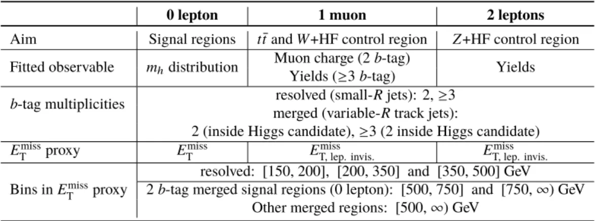
The likelihood includes all control and signal regions, as detailed in Table 2, where these regions are binned to increase the sensitivity and improve the determination of the normalisation factors for t t ¯ and W /Z +HF.

The signal regions are binned in the invariant mass of the Higgs boson candidate as defined in Section 5.

The choice of the binning in the signal regions is optimised to obtain the best expected sensitivity to the signal models addressed in this paper, while also keeping statistical uncertainties in each bin low.

The 1-muon control regions are binned in positive or negative muon charge in the case of the 2 b -tag regions. This improves the separation between t t ¯ and W +HF processes, as W +HF processes exhibit a charge asymmetry in pp collisions. Only inclusive event yields are used in the other regions, which are dominated by t¯ t , and for the 2-lepton control regions.

0 lepton 1 muon 2 leptons

Aim Signal regions tt¯andW+HF control region Z+HF control region Fitted observable m_hdistribution Muon charge (2b-tag)

Yields Yields (≥3b-tag)

b-tag multiplicities resolved (small-Rjets): 2,≥3 merged (variable-Rtrack jets):

2 (inside Higgs candidate),≥3 (2 inside Higgs candidate) E^miss

T proxy E^miss

T E^miss

T, lep. invis. E^miss

T, lep. invis.

Bins inE^miss

T proxy

resolved: [150, 200], [200, 350] and [350, 500] GeV

2b-tag merged signal regions (0 lepton): [500, 750] and [750,∞) GeV Other merged regions: [500,∞) GeV

Table 2: Event categories entering the combined fit of the model to the data. The discriminantm_hdenotes the mass of the light Higgs boson candidate and corresponds to either the di-jet massm_{j j} in the regions selecting two small-R jets or to the large-Rjet massm_Jfor the regions requiring a large-Rjet.

The nominal fit results are obtained by maximising the likelihood function with respect to all parameters.

Two different fit configurations are used: in the background-only profile likelihood fit, the parameters are determined in a fit to data assuming the presence of no signal. The second fit configuration instead allows for the presence of a specific signal, and is referred to as the model-dependent fit.

The test statistic q

is constructed using the profile likelihood [105]: q

= − 2 ln (L(µ, θ ˆˆ

)/L( µ, ˆ θ)) ˆ , where

µ ˆ and ˆ θ are the parameters that maximise the likelihood, and θ ˆˆ

are the nuisance parameter values

that maximise the likelihood for a given µ . This test statistic is used to measure the compatibility of

the background-only model with the observed data and to derive exclusion intervals using the CL

-

prescription [106].

7 Systematic uncertainties

Signal and background expectations are subject to statistical, detector-related and theoretical uncertainties, which are all included in the likelihood as nuisance parameters. Detector-related and theoretical uncertainties may affect the overall normalisation and/or shape of the simulated background and signal events.

Detector-related uncertainties are dominated by contributions from the jet reconstruction. Uncertainties on the jet energy scale (JES) for small- R jets [94] arise from the calibration of the scale of the jet and are derived as function of the jet p

, and also η . Further contributions emerge from the jet flavour composition and the pile-up conditions. The ‘category reduction’ scheme as described in Ref. [94] with 29 nuisance parameters is used. Uncertainties on the jet energy resolution (JER) depend on the jet p

and η and arise both from the method used to derive the jet resolution and from the difference between simulation and data [94], and they are included with eight nuisance parameters. Similarly, uncertainties on the jet energy resolution for large- R jets arise from the calibration, the flavour composition and the topology dependence [107]. Further uncertainties are considered on the large- R jet mass scale [107] and resolution [108].

Uncertainties due to the b -tagging efficiency on heavy-flavour jets including c -flavour jets are derived from t¯ t data [109, 110] and are represented by four nuisance parameters. Uncertainties are also considered for mistakenly b -tagging a light-flavour jet with nine nuisance parameters. These are estimated using a similar method as in Ref. [111].

Uncertainties on the modelling of E

T

are evaluated by considering the uncertainties on the jets included in the calculation and on the soft term scale and resolution [112]. The pile-up in simulation is matched to the conditions in data by a reweighting factor. Uncertainties of 4% on this reweighting factor are considered. The uncertainty in the combined 2015–2018 integrated luminosity is 1.7% [40], obtained using the LUCID-2 detector [113] for the primary luminosity measurements.

Scale factors, including their uncertainties, are calculated specifically for this analysis to correct the efficiency of E

T

triggers in simulation to that in data. The uncertainties on the scale factors are at most 1-2% for low E

T

values.

In the regions requiring the presence of leptons, uncertainties on the lepton identification and lepton energy/momentum scale and resolution are included. These are derived using simulated and measured events with Z → l

l

, J/ψ → l

l

and W → lν decays [96, 98].

The theoretical uncertainties are dominated by modelling uncertainties on the t t ¯ and Z +HF backgrounds.

For the t t ¯ and Wt processes, the impact of the parton shower and hadronisation model is evaluated by comparing the nominal generator setup with a sample interfaced to Herwig 7.04 [114, 115]. To assess the uncertainty on the matching of NLO matrix elements to the parton shower, the Powheg sample is compared with a sample of events generated with MadGraph5_aMC@NLO v2.6.2. For the Wt process, the nominal sample is compared with an alternative sample generated using the diagram subtraction scheme [73, 80]

instead of the diagram removal scheme to estimate the uncertainty arising from the interference with t¯ t production.

Uncertainties on V +jet processes arising from the modelling of the parton shower and the matching scheme are evaluated by comparing the nominal samples to samples generated with MadGraph5_aMC@NLO v2.2.2.

For the diboson processes, the uncertainties associated to the modelling of the parton shower, the hadron- isation and the underlying event are derived using alternative samples generated with PowhegBox [56–58]

and interfaced to Pythia 8.186 [116] or Herwig++.

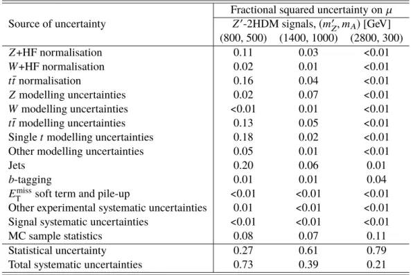
Source of uncertainty

Fractional squared uncertainty on µ Z

-2HDM signals, (m

, m

) [GeV]

(800, 500) (1400, 1000) (2800, 300)

Z +HF normalisation 0.11 0.03 <0.01

W +HF normalisation 0.02 0.01 <0.01

t¯ t normalisation 0.16 0.04 <0.01

Z modelling uncertainties 0.02 0.07 <0.01

W modelling uncertainties <0.01 0.01 <0.01

t¯ t modelling uncertainties 0.13 0.05 <0.01

Single t modelling uncertainties 0.18 0.02 <0.01

Other modelling uncertainties 0.05 0.01 <0.01

Jets 0.20 0.06 0.01

b -tagging 0.01 0.01 0.04

E

T

soft term and pile-up <0.01 <0.01 <0.01

Other experimental systematic uncertainties 0.01 <0.01 <0.01 Signal systematic uncertainties <0.01 <0.01 <0.01

MC sample statistics 0.08 0.07 0.11

Statistical uncertainty 0.27 0.61 0.79

Total systematic uncertainties 0.73 0.39 0.21

Table 3: Impact of the different sources of uncertainty for differentZ⁰-2HDM, with the masses of theZ⁰boson and theAboson given in the second row, expressed as fractional impact on the signal strength parameter. The fractional impact is calculated by considering the square of the uncertainty on the signal strength parameter arising from a given group of uncertainties (as denoted in the left column of the table), divided by the square of the total uncertainty on the signal strength parameter. Due to correlations, the sum of the different impacts of systematic uncertainties might not add up to the total impact of all systematic uncertainties.

For all MC samples, the uncertainties due to missing higher orders are estimated by a variation of the renormalisation and factorisation scales by a factor of two, while the PDF and α

uncertainties are calculated using the PDF4LHC prescription [117].

Table 3 gives the impact of the different sources of systematic uncertainties for selected signal models as evaluated in different model-dependent fits. The signal models with lower masses illustrate the impact of the systematic uncertainties in the resolved regions, while the models with larger mediator masses are more impacted by the merged regions. The theoretical uncertainties on the modelling of the t t ¯ background, the experimental uncertainties on the calibration of jets and the limited MC statistics show the largest impact.

8 Results

In a background-only profile likelihood fit to data in all regions, the post-fit background yields are

determined. The post-fit normalisation factors for t¯ t and for W +HF are found to be 0 . 93 ± 0 . 08 and

0 . 95 ± 0 . 14, respectively. For Z boson production in association with two (at least three) heavy-flavour jets

the normalisation factors are determined to 1 . 41 ± 0 . 09 (1 . 85 ± 0 . 24). An upward scaling of the Z +HF

background in comparison to the simulation was also observed in other studies [118], and was attributed

2E^missb-tag signal regions [150,200]GeV [200,350]GeV [350,500]GeV [500,750]GeV >750 GeV

T range

Z+HF 6470±310 7200±310 507±26 94±7 9.2±1.8

Z+light jets 72±15 137±29 18±4 4.5±1.0 1.17±0.30

W+HF 1590±210 1760±230 106±14 25±4 3.1±0.6

W+light jets 86±35 92±35 14±5 1.6±0.6 0.21±0.09

Single top-quark 570±260 570±260 21±10 2.6±1.9 0.10±0.16

tt¯ 4680±290 3280±240 76±9 11.4±1.6 0.38±0.08

Diboson 450±50 600±60 56±7 15.2±1.9 1.61±0.29

V h 151±10 202±12 26.6±1.8 5.6±0.5 0.68±0.12

tt¯+V/h 7.6±0.4 11.8±0.5 0.45±0.06 0.286±0.029 0.035±0.006 Total background 14070±110 13860±100 825±19 160±8 16.7±1.9

Data 14259 13724 799 168 19

Table 4: Background yields in comparison to data in the 2b-tag signal regions for differentE^miss

T ranges after a background-only fit to data. Statistical and systematic uncertainties are reported together.

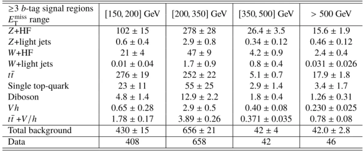
≥3b-tag signal regions [150,200]GeV [200,350]GeV [350,500]GeV >500 GeV E^miss

T range

Z+HF 102±15 278±28 26.4±3.5 15.6±1.9

Z+light jets 0.6±0.4 2.9±0.8 0.34±0.12 0.46±0.12

W+HF 21±4 47±9 4.2±0.9 2.4±0.4

W+light jets 0.01±0.04 1.7±0.9 0.8±0.4 0.031±0.026

tt¯ 276±19 252±22 5.1±0.7 17.9±1.8

Single top-quark 23±11 55±25 2.9±1.4 3.4±1.7

Diboson 4.8±1.4 12.9±2.2 1.8±0.4 1.26±0.31

V h 0.65±0.28 2.9±0.5 0.40±0.08 0.230±0.025

tt¯+V/h 1.78±0.17 3.89±0.26 0.371±0.035 0.78±0.08

Total background 430±15 656±21 42±4 42.0±2.8

Data 408 658 42 46

Table 5: Background yields in comparison to data in the≥3b-tag signal regions for differentE^miss

T ranges after a background-only fit to data. Statistical and systematic uncertainties are reported together.

to an underestimation of the g → b b ¯ rate in Sherpa. A larger scaling is observed in the region with ≥ 3 b -tagged jets, dominated by processes with more g → b b ¯ splittings.

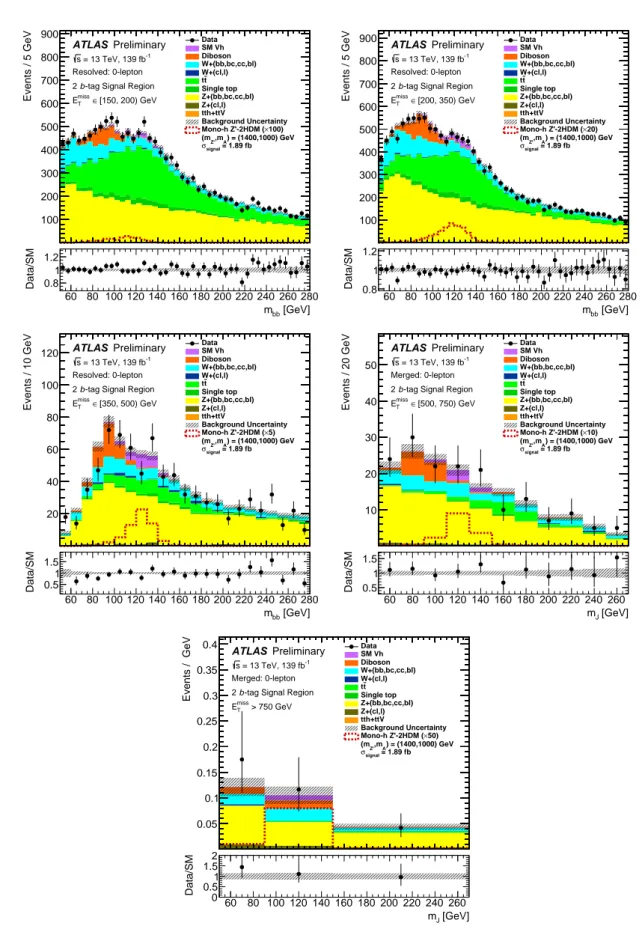
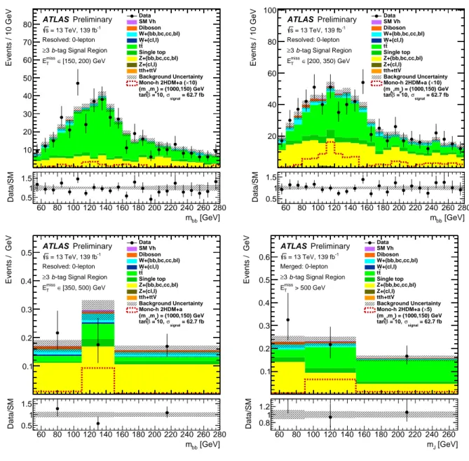
The distributions of the Higgs boson candidate mass m

after the background-only fit are shown in Figs. 3-4.

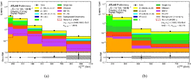
Tables 4 and 5 present the background estimates in comparison to the observed data. No significant deviation from SM expectations is observed, with the largest underfluctuation corresponding to a local significance of 2.3 σ , and the largest overfluctuation amounting to 1.6 σ . Figure 5 summarises the total yields in the signal regions as function of E

T

. The background prediction from simulation is scaled upwards in the fit for lower E

T

values, while the simulation agrees better with the data for large E

T

values.

60 80 100 120 140 160 180 200 220 240 260 280m_bb [GeV]

100 200 300 400 500 600 700 800 900

Events / 5 GeV

Data SM Vh Diboson W+(bb,bc,cc,bl) W+(cl,l)

t t Single top Z+(bb,bc,cc,bl) Z+(cl,l) tth+ttV

Background Uncertainty

×100) Mono-h Z'-2HDM (

) = (1400,1000) GeV ,mA

(mZ'

= 1.89 fb

signal

σ

ATLAS Preliminary = 13 TeV, 139 fb-1

s

Resolved: 0-lepton -tag Signal Region b

2

[150, 200) GeV

miss∈ ET

60 80 100 120 140 160 180 200 220 240 260 280 [GeV]

mbb

0.8 1 1.2

Data/SM

60 80 100 120 140 160 180 200 220 240 260 280m_bb [GeV]

100 200 300 400 500 600 700 800 900

Events / 5 GeV

Data SM Vh Diboson W+(bb,bc,cc,bl) W+(cl,l)

t t Single top Z+(bb,bc,cc,bl) Z+(cl,l) tth+ttV

Background Uncertainty

×20) Mono-h Z'-2HDM (

) = (1400,1000) GeV ,mA

(mZ'

= 1.89 fb

signal

σ

ATLAS Preliminary = 13 TeV, 139 fb-1

s

Resolved: 0-lepton -tag Signal Region b

2

[200, 350) GeV

miss∈ ET

60 80 100 120 140 160 180 200 220 240 260 280 [GeV]

mbb

0.8 1 1.2

Data/SM

60 80 100 120 140 160 180 200 220 240 260 280m_bb [GeV]

20 40 60 80 100 120

Events / 10 GeV

Data SM Vh Diboson W+(bb,bc,cc,bl) W+(cl,l)

t t Single top Z+(bb,bc,cc,bl) Z+(cl,l) tth+ttV

Background Uncertainty

×5) Mono-h Z'-2HDM (

) = (1400,1000) GeV ,mA

(mZ'

= 1.89 fb

signal

σ

ATLAS Preliminary = 13 TeV, 139 fb-1

s

Resolved: 0-lepton -tag Signal Region b

2

[350, 500) GeV

∈

miss

ET

60 80 100 120 140 160 180 200 220 240 260 280 [GeV]

mbb

0.5 1 1.5

Data/SM

60 80 100 120 140 160 180 200 220 240 260m_J [GeV]

10 20 30 40 50

Events / 20 GeV

Data SM Vh Diboson W+(bb,bc,cc,bl) W+(cl,l)

t t Single top Z+(bb,bc,cc,bl) Z+(cl,l) tth+ttV

Background Uncertainty

×10) Mono-h Z'-2HDM (

) = (1400,1000) GeV ,mA

(mZ'

= 1.89 fb

signal

σ

ATLAS Preliminary = 13 TeV, 139 fb-1

s

Merged: 0-lepton -tag Signal Region b

2

[500, 750) GeV

∈

miss

ET

60 80 100 120 140 160 180 200 220 240 260 [GeV]

mJ

0.5 1 1.5

Data/SM

60 80 100 120 140 160 180 200 220 240 260mJ [GeV]

0.05 0.1 0.15 0.2 0.25 0.3 0.35 0.4

Events / GeV

Data SM Vh Diboson W+(bb,bc,cc,bl) W+(cl,l)

t t Single top Z+(bb,bc,cc,bl) Z+(cl,l) tth+ttV

Background Uncertainty

×50) Mono-h Z'-2HDM (

) = (1400,1000) GeV ,mA

(mZ'

= 1.89 fb

signal

σ

ATLAS Preliminary = 13 TeV, 139 fb-1

s

Merged: 0-lepton -tag Signal Region b

2

> 750 GeV

miss

ET

60 80 100 120 140 160 180 200 220 240 260 [GeV]

mJ

0 0.51 1.5 2

Data/SM

Figure 3: Distributions of the Higgs boson candidate mass in the 2b-tag signal regions for differentE^miss

T ranges.

The background yields are obtained in a background-only fit to data. An example signal model from theZ⁰-2HDM