Max-Planck-Institut f¨ ur Physik
Search for Dark Matter with the
CRESST Experiment
Dissertation an der Fakult¨ at f¨ ur Physik der Technischen Universit¨ at M¨ unchen
vorgelegt von
Rafael Florian Lang
Max-Planck-Institut f¨ ur Physik (Werner-Heisenberg-Institut)
Search for Dark Matter with the CRESST Experiment
Rafael Florian Lang
Vollst¨ andiger Abdruck der von der Fakult¨ at f¨ ur Physik der Technischen Universit¨ at M¨ unchen zur Erlangung des akademischen Grades eines
Doktors der Naturwissenschaften genehmigten Dissertation.
Vorsitzender: Univ.-Prof. Dr. Alejandro Ibarra Pr¨ ufer der Dissertation:
1. Univ.-Prof. Dr. Lothar Oberauer 2. Hon.-Prof. Allen C. Caldwell, Ph.D
Die Dissertation wurde am 28. Oktober 2008 bei der Technischen Univer-
sit¨ at M¨ unchen eingereicht und durch die Fakult¨ at f¨ ur Physik am 4. Dezem-
ber 2008 angenommen.
In recent years cosmology became a quantitative science, predicting large quantities of Dark Matter (chapter 1). Astrophysical measurements also point toward such a dark component of our universe, being distributed on all scales from galaxy clusters to our own Milky Way (chapter 2). However, Dark Matter could so far not be observed directly (chapter 3).
The CRESST Experiment aims at the detection of Dark Matter particles on a laboratory scale. To this end, scintillating crystals are equipped with superconducting thermometers and cooled to a few millkelvin only. Hence particles can be detected calorimetrically. Using the information given by the scintillation allows to distinguish different kinds of particles, which in turn allows to suppress common radioactive backgrounds (chapter 4).
This work deals with the analysis of data attained. As a start, the employed methods are explained (chapter 5). Detailed investigations of the recorded spectra below a few 100 keV allow the identification of a variety of background sources (chapter 6).
The energy dependence of the scintillation light yield is of much rele- vance for the discrimination power of the experiment. For the first time a scintillator non-proportionality was shown to exist in CRESST detectors, as well as a differing behavior for electron and gamma events (chapter 7).
The possibility to use the light detectors themselves as an absorber in a Dark Matter search is briefly examined (chapter 8). The analysis of data to search for Dark Matter is exhaustively reported. Employing new parameters allows to isolate classes of relevant backgrounds (chapter 9).
The calculation of a limit on the Dark Matter scattering cross section is explained. An algorithm is developed that allows to make use of the data in an optimal way. Moreover, a new method to combine data from differ- ing detectors is presented. Finally, a limit on the coherent WIMP-nucleus scattering cross section from data taken during 2007 is given (chapter 10).
5
Die Kosmologie konnte sich in den letzten Jahren verst¨ arkt zu einer quanti- tativen Wissenschaft entwickeln und sagt eine große Menge der sogenannten Dunklen Materie voraus (Kapitel 1). Auch astrophysikalische Messungen deuten auf große Mengen einer solchen dunklen Komponente unseres Univer- sums hin, auf Skalen von Galaxienhaufen bis zu unserer Milchstraße (Kapi- tel 2). Allerdings entzieht sich die Dunkle Materie bislang jeder direkten Beobachtung (Kapitel 3).
Mit dem CRESST Experiment wird versucht, Teilchen der Dunklen Ma- terie im Labormaßstab nachzuweisen. Dazu werden szintillierende Kristalle mit supraleitenden Thermometern versehen und auf wenige tausendstel Kelvin abgek¨ uhlt. Im Falle einer Wechselwirkung k¨ onnen so Teilchen kalorimetrisch nachgewiesen werden. Der Nachweis des Szintillationslichtes erlaubt R¨ uckschl¨ usse ¨ uber die Teilchenart, was eine wesentliche Unter- dr¨ uckung allgemeiner radioaktiver Untergr¨ unde erm¨ oglicht (Kapitel 4).
Diese Arbeit besch¨ aftigt sich mit der Auswertung der im Experiment gewonnenen Daten. Die eingesetzte Methodik wird zun¨ achst erl¨ autert (Kapitel 5). Ausf¨ uhrliche Untersuchungen der gewonnenen Spektren im Energiebereich unterhalb weniger 100 keV erlauben die Identifizierung einer Vielzahl verschiedener Quellen (Kapitel 6).
Die Energieabh¨ angigkeit der Lichtausbeute ist f¨ ur das Diskriminierungs- potential von großer Bedeutung. In diesem Zusammenhang kann erstmals eine nichtproportionale Energieabh¨ angigkeit der Lichtausbeute ebenso wie unterschiedliche Reaktionen auf Elektronen- und Gammaereignisse in den CRESST Detektoren nachgewiesen werden (Kapitel 7).
Die M¨ oglichkeit, die eingesetzten Lichtdetektoren selbst als Absorber f¨ ur die Dunkle Materie einzusetzen, wird kurz behandelt (Kapitel 8). Die Verwertung der Daten zur Suche nach Dunkler Materie wird ausf¨ uhrlich dargestellt. Dabei k¨ onnen unter Einsatz neuer Parameter Klassen von rele- vanten Untergr¨ unden isoliert werden (Kapitel 9).
Die Berechnung einer oberen Schranke auf den Wirkungsquerschnitt der Dunklen Materie wird ausf¨ uhrlich dargelegt. Insbesondere wird ein Algo- rithmus entwickelt, mit welchem die gewonnenen Daten im Hinblick auf Ihre Aussagekraft optimal verwertet werden k¨ onnen. Desweiteren wird eine Methode zur Kombination der Daten verschiedener Detektoren vorgestellt.
Schließlich wird mit den 2007 gewonnenen Daten eine obere Schranke f¨ ur den koh¨ arenten WIMP-Nukleon Wirkungsquerschnitt angegeben (Kapitel 10).
6
Abstract / ¨ Uberblick 5
I Dark Matter 13
1 Non-Baryonic Matter 15
1.1 The Friedman Universe . . . . 15
1.1.1 An Introductory Comment . . . . 15
1.1.2 The Friedman-Lemaˆıtre-Robertson-Walker Metric . . 16
1.1.3 General Relativity . . . . 16
1.1.4 Various Densities . . . . 17
1.2 Nucleosynthesis . . . . 17
1.3 The Cosmic Microwave Background . . . . 19
1.4 Additional Observations . . . . 22
2 What and Where to Search 25 2.1 A Historical Perspective . . . . 25
2.2 Weakly Interacting Massive Particles . . . . 26
2.3 Galaxy Clusters . . . . 28
2.4 The Local Group . . . . 30
2.5 Spiral Galaxies . . . . 30
2.6 The Milky Way . . . . 32
2.7 The Solar System . . . . 35
II Detection Experiments 37 3 Hunting Dark Matter 39 3.1 Collider Experiments . . . . 39
3.2 Annihilation Searches . . . . 39
3.2.1 meV Photons . . . . 40
3.2.2 511 keV Gammas . . . . 41
3.2.3 Galactic GeV Gamma Rays . . . . 42
3.2.4 Extragalactic GeV Gamma Rays . . . . 43
3.2.5 TeV Gamma Rays . . . . 43
3.2.6 Positrons . . . . 44
7
3.2.7 Antiprotons . . . . 45
3.2.8 Antideuterons . . . . 45
3.2.9 Neutrinos . . . . 46
3.3 Direct Scattering . . . . 47
3.3.1 Astro- and Geophysical Constraints . . . . 47
3.3.2 Low Energies . . . . 48
3.3.3 Low Rates . . . . 48
3.3.4 Interaction Modes . . . . 49
3.3.5 Expected Recoil Spectrum . . . . 50
3.3.6 Signal Identification . . . . 54
3.4 Scattering Experiments . . . . 57
3.4.1 Ionization Detectors: Si/Ge . . . . 58
3.4.2 Common Scintillators: NaI/CsI . . . . 58
3.4.3 Cryogenic Ionization Detectors . . . . 59
3.4.4 Liquid Noble Elements . . . . 60
3.4.5 Bubble Chambers . . . . 60
3.4.6 Gaseous Detectors . . . . 61
4 CRESST 63 4.1 Shielding . . . . 63
4.1.1 Muons . . . . 64
4.1.2 Radon . . . . 64
4.1.3 Gammas and Electrons . . . . 66
4.1.4 Neutrons . . . . 68
4.2 Layout of the Experiment . . . . 71
4.2.1 The Cryostat . . . . 71
4.2.2 Setup . . . . 71
4.2.3 Experimental Volume . . . . 72
4.3 CRESST Detectors . . . . 74
4.3.1 Cryogenic Calorimeters . . . . 74
4.3.2 CRESST-I . . . . 75
4.3.3 Scintillating Crystals . . . . 76
4.3.4 Light Detector . . . . 77
4.3.5 Detector Modules . . . . 78
4.3.6 Reflective Foil . . . . 80
4.3.7 Model of Pulse Formation . . . . 80
4.4 Data Taking . . . . 83
4.4.1 SQUID Based Readout . . . . 83
4.4.2 Data Acquisition . . . . 85
4.4.3 Heater Pulses . . . . 85
III Data Analysis 89 5 Detector Operation and Data Analysis 91 5.1 Detector Operation . . . . 91
5.1.1 Transition Curve Measurement . . . . 91
5.1.2 Operating Point . . . . 93
5.1.3 Stability Control . . . . 93
5.2 Pulse Parameters . . . . 93
5.2.1 Main Parameters . . . . 94
5.2.2 Life Time . . . . 94
5.3 Pulse Height Evaluation . . . . 95
5.3.1 Creating a Standard Event . . . . 96
5.3.2 How Many Events to Include . . . . 97
5.3.3 The Truncated Fit . . . . 98
5.3.4 The Correlated Truncated Fit . . . . 99
5.4 Calibration . . . . 99
5.4.1 Cobalt Calibration . . . 100
5.4.2 Calibration With Heater Pulses . . . 100
5.4.3 Time Variations . . . 102
5.4.4 Light Detectors . . . 103
5.4.5 Amplitude Cut . . . 103
6 Spectral Features 105 6.1 Co-57 Calibration . . . 105
6.1.1 The Plain Spectrum . . . 105
6.1.2 Escape Peaks . . . 106
6.1.3 Coincident Events . . . 108
6.2 Background Spectra . . . 111
6.2.1 Pb-210 . . . 112
6.2.2 Ac-227 . . . 115
6.2.3 Pb-212 . . . 116
6.2.4 Activated Tungsten . . . 117
6.2.5 Ca-41 . . . 120
6.2.6 Ca-45 . . . 121
6.2.7 Copper Fluorescence . . . 121
6.2.8 11.5 keV . . . 122
6.2.9 Lu-176 . . . 122
7 Quenching 127 7.1 Quenching . . . 127
7.1.1 Quenching of Various Nuclei . . . 127
7.1.2 Linearity . . . 129
7.2 Position Dependence . . . 129
7.3 Scintillator Non-Proportionality . . . 133
7.3.1 The Model of Rooney and Valentine . . . 133
7.3.2 Observed Non-Proportionality . . . 133
7.4 Gamma and Electron Quenching . . . 135
7.4.1 Pb-210 . . . 136
7.4.2 Ta-179 . . . 138
7.4.3 W-181 . . . 139
7.4.4 More Physics in Run 30 . . . 139
8 Light Detector as Target 143
8.1 Low Energy Interactions . . . 143
8.2 BE13 in Run 28 . . . 144
8.2.1 Data Reduction . . . 144
8.2.2 Energy Estimation and Resolution . . . 145
8.2.3 Observed Spectrum . . . 148
8.3 Calculating a Limit . . . 150
8.3.1 Isothermal Milky Way Halo . . . 150
8.3.2 WIMPs in the Solar System . . . 152
9 Dark Matter Analysis 155 9.1 Blind Analysis . . . 155
9.2 Cuts . . . 157
9.2.1 Pathological Pulses . . . 157
9.2.2 Stability Cut . . . 157
9.2.3 Amplitude Cut . . . 161
9.2.4 Light Detector Cut . . . 161
9.2.5 Right-Minus-Left-Baseline Cut . . . 161
9.2.6 Quality of Fit . . . 164
9.2.7 Effect of the Cuts . . . 164
9.3 Unblinding . . . 170
9.3.1 Bowler Hats . . . 171
9.4 Other Data Sets . . . 174
9.5 Discussion of Low Light Yield Events . . . 175
9.5.1 External Neutrons . . . 175
9.5.2 Other Modules . . . 177
9.5.3 Muon Induced Events . . . 177
9.5.4 Alpha Decays . . . 178
9.5.5 Cracks in the Crystals . . . 178
9.5.6 Thermal Relaxations . . . 178
9.5.7 WIMPs . . . 179
9.6 Phonon Detector Resolution . . . 179
9.7 Light Detector Resolution . . . 182
9.7.1 Excess Light Events . . . 183
9.7.2 Determination of the Resolution . . . 185
9.7.3 Validating the Method with Simulation . . . 189
9.8 Po-210 Surface Events . . . 192
9.8.1 Po-210 in Run 27 . . . 192
9.8.2 Po-210 in Run 30 . . . 193
10 Calculating Limits 197 10.1 Nuclear Recoil Band . . . 197
10.2 Energy Dependent Acceptance . . . 199
10.2.1 The Objective Function . . . 199
10.2.2 Varying the Acceptance Region . . . 201
10.2.3 New Frontiers . . . 202
10.3 Calculating a Limit . . . 204
10.3.1 Two Parameter Limits . . . 204
10.3.2 The Yellin Methods . . . 204
10.3.3 The Maximum Gap Method . . . 205
10.3.4 The Optimum Interval Method . . . 205
10.4 Combining Detectors . . . 207
10.4.1 Two-Parameter Limits . . . 207
10.4.2 Frequentist vs. Bayesian . . . 207
10.4.3 Energy Transformation . . . 208
10.5 Limit from Run 30 . . . 209
11 Outlook 211 A Inflation 213 B Surface Treatment 215 B.1 Safety Notices . . . 215
B.2 Cleaning Copper . . . 215
B.3 Cleaning Other Materials . . . 218
C Main Parameters 219 D Absorption of Photons 221 E Time Differences in a Poisson Process 223 F Cut Defining Histograms 225 G Dark Events 229 H Bowler Events 235 I Alternative Resolution Extraction 237 I.1 The Method . . . 237
I.1.1 Extracting the Band . . . 237
I.1.2 Extracting the Resolution . . . 237
I.2 Validating the Method . . . 239
I.3 Applying the Method . . . 240
Acknowledgments 243
Bibliography 245
Was ists, daß ich nun in dir
Von sanfter Wollust meines Daseins gl¨ uhe?
Einem Kristall gleicht meine Seele nun,
Den noch kein falscher Strahl des Lichts getroffen;
Zu fluten scheint mein Geist, er scheint zu ruhn, Dem Eindruck naher Wunderkr¨ afte offen,
Die aus dem klaren G¨ urtel blauer Luft Zuletzt ein Zauberwort vor meine Sinne ruft.
Eduard M¨ orike
Dark Matter
13
The Need for Non-Baryonic Matter
Intent: The work done within the framework of this thesis is devoted to the search for a new form of matter. This chapter introduces the need for such non-baryonic matter from various cosmological observations. In particular, Big Bang nucleosynthesis and observations of the cosmic mi- crowave background radiation independently lead to the same conclusion:
All the atoms make up only 4% of the energy density of the universe. We will see that five times more mass is hidden in the universe in an unknown form: the Dark Matter.
Organization: Section 1.1 gives an overview over contemporary cosmol- ogy, and introduces the notion of energy densities. Based on measure- ments of the abundances of light elements as well as the cosmic microwave background radiation, the following sections 1.2 and 1.3 respectively ex- plain why baryonic matter can only contribute a small fraction to the total matter density. Finally, in section 1.4, other measurements are re- marked at, and the findings are summarized in a coherent picture.
1.1 The Friedman Universe
1.1.1 An Introductory Comment
In cosmology, one usually works in the so-called comoving coordinate system. We are familiar with this peculiar concept of coordinates when we think of the latitudes and longitudes on the earth globe (radius R ⊕ ). Almost at the north pole, for example, moving in longitude φ by one degree to the east implies traversing a much smaller distance than moving one degree to the east from M¨ unchen. The physical distance ds traversed is related to the coordinate distance (dθ, dφ) by a metric
ds 2 = R ⊕ 2 dθ 2 + sin 2 θ dφ 2
(1.1) which tells us how to calculate physical distances from our coordinates (θ, φ).
In the example, we have sin 2 θ → 0 on the north pole, so the physical distance ds traversed becomes very small.
15
1.1.2 The Friedman-Lemaˆıtre-Robertson-Walker Metric The cosmological principle states that the universe is everywhere the same, a very appealing postulate indeed in the light of the copernican history of science. More precisely, the principle assumes homogeneity and isotropy of the universe at scales l 100 Mpc, which is the typical scale of clusters of galaxies such as our Local Group. We will see in section 1.3 that this indeed agrees very well with observations. The generic metric for such a universe is the Friedman-Lemaˆ ıtre-Robertson-Walker metric (labeled also using any subset of these four names, depending on regional preferences):
ds 2 = c 2 dt 2 − a(t) 2
dr 2
1 − kr 2 + r 2 dθ 2 + r 2 sin 2 θ dφ 2
. (1.2) For constant r = R ⊕ this metric compares nicely to equation 1.1. In ad- dition, it contains a free function a(t) called the scale factor, and a free parameter k, describing the curvature of space-time. In section 1.3 we will also see that all observations point toward our universe being spatially flat (unless warped by gravitating bodies like galaxies), in which case k = 0.
Thus, the metric describing our universe is very simply ds 2 = c 2 dt 2 − a(t) 2 dx 2 + dy 2 + dz 2
(1.3) which is almost the Minkovsky metric, except that the spatial component has the scale factor in. We set the value a 0 ≡ a(t = today) := 1.
It was already in 1912 that Slipher discovered the apparent receding radial movement of the galaxies [1, 2], but only in 1929 that Hubble claimed his now famous law [3] of the expansion of the universe. Today, what we mean with the notion that the universe is expanding simply means that the scale factor a(t) is increasing with time. For a nice review on this matter see reference [4].
1.1.3 General Relativity
Within the framework of General Relativity, the time evolution of the scale factor a(t) is determined by the ten fundamental Einstein equations [5]
G µν − Λg µν = 8πG
3 T µν (1.4)
with the Einstein tensor G µν describing the curvature of space-time, a cosmological constant Λ, the metric tensor g µν as defined in equation 1.3, Newton’s constant G, and the stress-energy tensor T µν describing the density and flux of energy and momentum in space-time.
Inserting our metric 1.3 into these equations decouples the individual components, since the metric is diagonal. Solving the time-time-component (µ = ν = 0) of equations 1.4 yields the first Friedman equation, derived already in 1922 [6]:
H 2 (t) :=
a(t) ˙ a(t)
2
= 8πG
3c 2 % + c 2 Λ
3 − c 2 k
a 2 (t) . (1.5)
Here, % ≡ T 00 is the energy density of the universe, and H is called the Hub- ble parameter, with H 0 ≡ H(t = today) = (70.1 ± 1.3) km s −1 Mpc −1 [7]
called the Hubble constant for historic reasons. It is this simple equa- tion 1.5 that describes the evolution of the expansion of the universe.
1.1.4 Various Densities
With the Friedman equation 1.5 at hand, it is enough to measure the terms on the right hand side today to know the past and future evolution of the universe. To this end, it is customary to divide the equation by H 0 to get
8πG
3c 2 H 0 2 % + c 2 Λ
3H 0 2 − c 2 k
a 2 H 0 2 = 1. (1.6)
We define the critical density
% critical := 3c 2 H 2 (t)
8πG (1.7)
which today has a value of % critical,0 ≈ 5 keV/cm 3 , corresponding to about 5 protons/m 3 . In cosmology it is customary to express the density of a species i not in g/cm 3 or the like, but as fraction of the critical density Ω i := % i,0 /% critical,0 . The Friedman equation is then simply
Ω matter + Ω Λ − Ω curvature = 1 (1.8)
or, if we allow a more detailed division of species, such as Ω baryons or Ω neutrinos , it reads
X
i
Ω i = 1. (1.9)
The following sections summarize the most important measurements of the various energy densities Ω i , based on the four fields of nucleosynthesis, cos- mic microwave radiation, structure formation, and supernovae.
1.2 Nucleosynthesis
After the Big Bang, neutrons and protons interact and form deuterium, which is again photodissociated by the ambient cosmic background radia- tion. After about 4 minutes, the temperature of the universe drops below T ≈ 80 keV/k B ≈ 10 9 K, and photodissociation is no longer significant. This is when Big Bang nucleosynthesis starts: Deuterium can now be fused into tritium, helium, and even lithium. Once the neutrons are all used up, we are left with charged particles only (the nuclei), so the coulomb barrier puts an end to nucleosynthesis at temperatures of T ≈ 30 keV/k B , at about 24 minutes after the Big Bang.
For the fraction of baryons that end up in helium (called the helium
mass fraction), the situation is very simple: Helium is energetically very
Figure 1.1: The abundances of light elements during Big Bang nucleosyn- thesis, as function of the baryon-to-photon ratio η 10 , or directly the baryon density Ω baryons = η 10 /137 [8]. Curves are shown for the four lightest ele- ments. The double lines represent the uncertainties due to nuclear physics processes, while the strictly horizontal bars are measurements including sta- tistical errors. This points toward a baryon density of only Ω baryons ≈ 0.04.
Tritium is not shown since it decays with a half-live time of only 12 years into 3 He. Plot based on data from [9].
favored, so to first order, all neutrons end up in 4 He. This means that the helium mass fraction is rather insensitive to the baryon density, but depends mainly on the initial ratio n/p at the time nucleosynthesis starts [9]. More precisely, with an initial n/p ≈ 1/7 (from Boltzmann statistics given the different masses of protons and neutrons), this allows for one helium nucleus per 12 hydrogen nuclei, so we expect to end up with about 25% of the mass of baryons in the form of 4 He, and the rest in hydrogen (figure 1.1).
For higher order effects, we can have a look at deuterium, where things are different. The higher the baryon density, the faster deuterium is fused into more heavy elements, so that after nucleosynthesis, we end up with a lower deuterium abundance. In fact, the deuterium abundance is a very sensitive measure of the baryon density at the time of nucleosynthesis, and consequently, the deuterium curve in figure 1.1 is rather steep. Deuterium is the baryometer of choice since it is only destroyed in the course of the evolu- tion of the universe, or the evolution of a star, but never enduringly created.
This is due to the low binding energy of deuterium, and it keeps systematic
uncertainties small: One can get a handle on the chemical evolution of stars
or nebulae by probing higher mass elements, and in regions where there was
hardly any chemical evolution at all, the deuterium abundance will be very close to the primordial one.
Also, observations of the abundances of 3 He and 7 Li can be used to get a handle on the baryon density as indicated in the figure. The values for Ω baryons derived from the deuterium abundance (Ω baryons = 0.047 ± 0.003) and from helium-3 (Ω baryons = 0.041 +0.016 −0.010 ) agree very well, with higher uncertainties and a tendency toward lower baryon densities for the abundances derived from helium-4 and lithium [9]. This is our first glimpse of what is to come, namely that the matter we know so dearly makes up only a small fraction of the energy content of the universe, as we have seen from the Friedman equation 1.8 that P
Ω i needs to add up to one.
1.3 The Cosmic Microwave Background
The cosmic microwave background (CMB) was discovered by Penzias and Wilson in 1964 [10] and quickly interpreted to be the echo of the Big Bang [11]. It was emitted when the universe was about 380,000 years old, when, at a temperature of T ≈ 0.3 eV/k B , electrons and protons combined to form neutral hydrogen. Thereafter, the primordial plasma became trans- parent for the photons to travel freely, so the apparent cosmic microwave background sphere is sometimes called the surface of last scattering.
What we can observe as the cosmic microwave background is only those photons that reach us precisely today, so we can see neither beyond the surface of last scattering, nor see the whole universe, but only a (possibly very small) slice of it.
Figure 1.2: The most perfect black body spectrum ever observed: The cos- mic microwave background. Shown are data together with a fit to a black body spectrum with T = 2.728 K: The error bars are incredibly small. Plot from [12].
Figure 1.2 shows the spectrum of the cosmic microwave background,
as measured by the FIRAS instrument on board the COBE satellite [12].
The cosmic microwave background is the most perfect Planck radiator we know, with its temperature today being pinned down to T CMB = (2.725 ± 0.001)K = 2 × 10 −4 eV/k B . From this, the energy density of photons today follows directly as Ω γ = (5.026 ± 0.001) × 10 −5 [8].
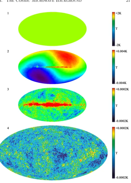
More information can be gained by looking very closely at this spec- trum [14], and one can see temperature fluctuations at the level of ≈ 10 −5 , see figure 1.3. What we see [15] as the structure in the cosmic microwave background is gravitational redshifting of the photons (Sachs-Wolfe ef- fect [16]) as they decouple from matter at the surface of last scattering.
This is an accurate probe of the matter distribution at that time. Thus by analyzing the structure in the cosmic microwave background, one can infer the distribution of gravitating matter in the early universe. To this end, one decomposes the observed picture into spherical harmonics in order to do some quantitative analysis on it, see figure 1.4. Some thoughts on why we can observe these variations at all, given that each multipole is an average over many modes, and given the universe is not bounded, are elaborated in appendix A.
Various parameters can be extracted from a combined fit to the cosmic microwave background spectrum. The densities that the microwave back- ground is most sensitive to are:
The curvature Ω curvature : In an open universe, the peaks would appear on smaller angular scales, since the geodesics pointing from us to the surface of last scattering are bent together (they are convex). By 2000, it was clear from BOOMERANG data that the universe is flat [19], and with the precision measurements of WMAP we can now put a tight limit of −0.0175 < Ω curvature < +0.0085 [15]. So, as promised in section 1.1.2, the universe really is flat.
The total matter density Ω matter : As one decreases the matter density, gravitational wells are more easily decaying. Then photons traveling on the way to us can gain more energy falling in these wells than they loose climbing out again (integrated Sachs-Wolfe effect). This decay might happen due to the presence of Dark Energy, massive neu- trinos, or something involving lots of radiation and little mass close to the time of last scattering. As observable, the effect increases all odd peaks in the power spectrum. So by looking at the relative size of the peaks one can get an excellent handle on the matter density. The five year data from WMAP constrains Ω matter = 0.257 ± 0.013 [17].
The baryon density Ω baryons : Gravity pull baryons together, but radi-
ation pressure drives them apart. This causes so-called baryon-
acoustic oscillations which leave their imprint in the cosmic mi-
crowave background’s power spectrum. Raising the baryon density
increases the peak height of the first peak but decreases the height
of the second peak, very much like in the case of a driven harmonic
oscillator when reducing the frequency of the driving force. Indeed,
Figure 1.3: 5 year WMAP observation of the cosmic background tempera-
ture, in galactic coordinates. (1) The radiation is highly uniform over the
whole sky. (2) A dipole structure emerges at a much finer temperature scale
(shown on the right). It is caused by the dipole from the movement of the
sun through the rest frame of the background radiation, and in galactic co-
ordinates shows up as this yin-yang-like pattern. (3) Subtracting the dipole
(and going to a finer temperature scale) the emission from the Milky Way
becomes visible. (4) Subtracting this emission (based on estimates from
the side bands of the radiation as well as on results of extensive modeling)
the cosmic microwave background anisotropy emerges. Figure with pictures
taken from [13].
Figure 1.4: The angular power spectrum of the cosmic microwave back- ground radiation. Shown are both binned data points from WMAP and other experiments (with error bars including cosmic variance), as well as unbinned data points from WMAP in gray. The simple cosmological model described here is capable of reproducing all observed features to very high accuracy, as shown by the best fit curve. Figure based on plots in [17]
and [18].
in the plasma, a large baryon density corresponds to a small speed of sound and thus small frequencies, so the analogy really holds. Today, the best way to measure the baryon density is to measure the speed of sound by means of the cosmic microwave background, and from the five year WMAP data one gets Ω baryons = 0.0463 ± 0.0013 [17].
Also the Dark Energy density can be inferred from observations of the cosmic microwave background [17] to be about Ω Λ = 0.74 ± 0.03, and the neutrino density is at most Ω ν < 0.028. Now, these densities do indeed add up to unity as required by the Friedman equation, and an independent calculation in which the total density is allowed to deviate from unity (thus violating either General Relativity or the copernican assumption of homo- geneity and isotropy) also shows that P
i Ω i = 1.0052 ± 0.0064 [15], another confirmation of our universe obeying the simple laws described. But we see again that a substantial fraction Ω matter − Ω baryons − Ω ν ≈ 0.18 of the universe is made from a form of matter we do not yet know.
1.4 Additional Observations
Taking the cosmic microwave background data alone to constrain the cos-
mological parameters leads to some degeneracies. Adding other indepen-
dent data sets can help to measure these parameters with even higher accu- racy [20, 21].
The structure we live in today evolved from the tiny fluctuations in the cosmic background. Modeling this evolution is obviously highly non- linear at later times and thus requires large computational efforts. But the combination of both such computer simulations (e.g. the Millennium Simulation [22]) as well as observations of the large scale structure of the universe today (e.g. from the Sloan Digital Sky Survey [23]) allows to independently constrain the cosmic parameters to Ω matter = 0.26 ± 0.03 and Ω baryons = 0.041 ± 0.008 [24, 25].
Figure 1.5: Combined constraints on the baryon fraction Ω baryons /Ω matter
as function of the total mass density Ω matter from the various observations discussed here: Deuterium and 3 He abundance and Big Bang nucleosynthesis in cyan and violet, respectively [9] (central line and 1σ contour), the WMAP 5 year observation of the cosmic microwave background [17] in green and the Sloan Digital Sky Survey in orange [24, 26], both with their 1σ and 2σ contours.
Today, the accepted model is that of hierarchical structure forma- tion, in which small structures merge to form larger and larger struc- tures [27]. It is known since early times of observational cosmology [28]
that structure formation requires large amounts of matter to be made from
heavy particles that do not interact with photons, a component dubbed cold
Dark Matter. In contrast, the density of light particles (e.g. neutrinos) is
restricted to Ω ν < 0.01 and by far not enough to explain all of the matter
content of the universe.
For completeness, observations of Supernovae of type IA shall be noted. These objects are believed to have intrinsically the same true mag- nitude. From their observations one can infer the Hubble diagram to high distances, yielding a good handle especially on the Dark Energy parameter Ω Λ , which is very useful given the degeneracy of measurements of the cosmic microwave background alone.
Figure 1.5 summarizes the deduced parameters of the different obser- vations discussed above, in the Ω baryons /Ω matter versus Ω matter plane. The observations are all independent from one another, but they are all con- sistent in their outcome [7]: Baryonic matter is only a small fraction Ω baryons = 0.0462±0.0015 of a larger part Ω matter = 0.233±0.013 which con- sists mainly of matter in an unknown form! This non-baryonic matter must not interact with photons, or else we would have seen it in some wavelength or another, so we call it the Dark Matter.
At this stage, a warning is advisable. Astronomers sometimes call things
like planets, dust, or black holes also by the name of Dark Matter. However,
in this thesis, the term is used in the more restrictive meaning, referring to
non-baryonic matter only. It is the central goal of this work to get closer to
the answer of what this Dark Matter is made of.
What and Where to Search
Intent: Now that we have seen that most of the matter in the universe is of unknown form, we should set out to explore this new frontier. This chapter will introduce ideas about what this Dark Matter might be made of, and we will see where we can hope to find it. In particular, there is evidence for a significant component of non-baryonic Dark Matter in our own Milky Way, so laboratory searches on Earth may unravel this mys- tery. Key parameters of the local Dark Matter distribution are presented.
Organization: After a quick motivation from an historical perspective in section 2.1, section 2.2 introduces the idea of Weakly Interacting Massive Particles to explain non-baryonic Dark Matter. In the remainder of this chapter, sections 2.3 to 2.7 discuss what we know about Dark Matter, starting from megaparsec galaxy cluster scales down to the 10 µpc scale of our Solar System.
2.1 A Historical Perspective
We have seen that a large fraction Ω darkmatter ≈ 0.18 of the content of the universe is matter in a form not yet known to us. This leaves us with the daunting task of searching for something Out There that remains invisible.
But this is not an impossible thing to do at all, as a historical remark might help to realize. The first predictions of non-luminous matter from observa- tions of gravitating systems were made already in the 19th century. From detailed observations of Sirius, F. Bessel predicted in 1844 the existence of an unobserved companion [29, 30], which was then discovered as Sirius B in 1862 by A. Clark [31]. From perturbation calculations on the orbit of Uranus, J. Adams in 1845 and U. Leverrier in 1846 predicted the existence of an eighth planet. Thus Neptune was discovered by J. Galle in 1846 already during the first night he had looked for it, and on the very spot predicted by theory [32, 33]. And of course one could continue with this story, perhaps mentioning the experimental detection of the neutrino [34, 35], and eventu- ally coming to a point where we know of having a black hole at the center of the Milky Way [36]. This should encourage us to go on with the quest for non-baryonic Dark Matter.
25
2.2 Weakly Interacting Massive Particles
Following reference [37], let us assume this non-baryonic Dark Matter is made from a new particle species χ. Constraints are placed on these particles by various experiments and observations; see reference [38] for a review rich in primary references.
From structure formation (section 1.4) we know that these particles have to be much more massive than neutrinos. In the early universe, when T m χ , these particles will be in thermal equilibrium. This means that they are present in some number density n χ , but constantly produced and destroyed in reactions χ χ ¯ ↔ f f ¯ , where f is some other particle. The annihilation reaction will take place with some characteristic reaction rate Γ = hσ A vi n χ where hσ A vi is the thermally averaged annihilation cross sec- tion σ A given a relative velocity v.
Another time scale is set by the Hubble expansion of the universe, namely the expansion rate H(t) ≡ a(t)/a(t). As the universe expands, the ˙ χ par- ticles will encounter themselves less and less often, so at some point, the annihilation reactions will no longer be possible. We say the particle will freeze out. After freeze out, the number density n χ in a comoving volume will stay constant, provided only the particle is stable and no other signif- icant production or destruction processes exist. The results from a more detailed numerical analysis, solving the Boltzmann equation in the early universe for n χ , leads to the prediction shown in figure 2.1.
Given the abundance of particles Ω χ , one can now predict the mass and cross section for these new Dark Matter particles χ as thermal relics of the early universe (e.g. [39]):
Ω χ ≡ n χ m χ c 2
% critical,0
≈ 6 × 10 4 pb km/s
hσ A vi . (2.1)
Given today’s value for Ω darkmatter , and setting Ω χ ≈ Ω darkmatter , we then get
hσ A vi ≈ 3 × 10 5 pb km/s (2.2)
from purely cosmological arguments.
If we turn to particle physics for a moment, the probability for the an- nihilation is given by Fermi’s Golden Rule,
hσ A vi = 2π
~
f f ¯
H ˆ |χ χi ¯
2
% f (2.3)
with matrix element f f ¯
H ˆ |χ χi ¯ and density of final states % f . Let the χ particles decay into N relativistic particle species. The energy E f available in the final state is then simply E f = m χ c 2 , and the density of final states is
% f = N 8π √ 2
(2π~c) 3 E f 2 . (2.4)
Figure 2.1: Left: The primordial number density n χ as function of the tem- perature of the universe T , scaled to the mass m χ of the particle; hence time progresses to the right. At first, the density follows the Boltzman-suppressed solid line. But at some point annihilation is no longer possible, the number density per comoving volume remains constant, and the particle is said to be frozen out. The higher the value for the thermally averaged annihilation cross section hσ A vi, the longer χ particles can annihilate, and the lower the relic abundance n relic . Figure based on the one from [39]. Right: Taking this production mechanism into account (results in dark blue), the observed Dark Matter density Ω darkmatter (in light blue) can be used to loosely con- strain the allowed mass range for the new particles, if they are to be a dominant component. In particular, a large window around masses typical for the weak interaction remains. Figure based on similar plots in [37, 40].
Note that loopholes exist that may modify this simple picture, see e.g. [41].
For a hypothetical new particle χ that is typical for the weak interaction, we would expect m χ ∼ O(10 GeV/c 2 ) like for the gauge bosons, and for the matrix element we can estimate
f f ¯
H ˆ |χ χi ∼ ¯ G Fermi = ( ~ c) 3 × 1.2 × 10 −5 GeV −2 . Plugging this in equation 2.3 (~c = 197 MeV fm), we would expect
hσ A vi ∼ 1 × 10 6 pb km/s (2.5)
if our new electroweak particles are the dominant component of Dark Matter.
This is a very curious number, and it came as a big surprise [42] that it is close to the cosmological number, equation 2.2. It is by no means clear why those completely independent estimates, one purely cosmological, the other coming from particle physics, should have anything to do with each other. What is more, many models exist as extension to the standard model of particle physics, that do predict particles with such properties.
Since these models are motivated by completely independent thoughts, this
makes this connection an intriguing argument in favor of this new particle.
Of course all this might just be a coincidence, but it is often taken as a hint on what to search for: thermal relic particles. They have a large mass and a cross section that is typical for the electroweak interaction, and are therefore called Weakly Interacting Massive Particles, or WIMPs for short. The CRESST experiment aims to detect such particles.
Let us examine in the following chapters, in a few examples from large to small scales, where in the universe we may expect Dark Matter, possibly in the form of WIMPs.
2.3 Galaxy Clusters
Figure 2.2: A Sloan/Spitzer image of the Coma cluster (Abell 1656), ex- tending many Mpc in space [43]. Almost everything on this picture is a galaxy, including the faint green dots. The few stars in the image can be told by the faint rays they have, caused by interference on the telescope’s secondary mirror support structure.
In a stable system of galaxies, kinetic energy T and potential energy V balance and are related via the virial theorem
2T = −V. (2.6)
One can thus infer the total mass m e.g. of a galaxy cluster by measuring the velocities of the galaxies in the cluster, yielding T and hence V with the radius of the cluster, and therefore m. From such observations of the coma cluster (see figure 2.2), F. Zwicky argued already in 1933 that there had to be 400 times more mass than is seen as luminous and coined the term Dunkle Materie to describe this discrepancy [44]. Denoting the mass of the sun as M , modern values for the Coma cluster are a total mass of 1.6 × 10 15 M [45], but the total mass of the gas and stars only adds up to about 2.4 × 10 14 M [46]. This ratio is rather typical, most clusters have 50 to 100 times more mass than inferred from their luminosity alone [47].
In 2006, a direct observational evidence for Dark Matter was found by observations of the galaxy cluster 1E0657-558, the Bullet Cluster [48]. The Bullet Cluster consists of two Clusters of galaxies which passed through each other some time in the past, as can be inferred from their proper motions.
Picture 2.3 shows the cluster as seen by three different data sets.
Figure 2.3: The Bullet Cluster, from [48]. Left: Black and white is an optical image, showing the galaxies. Weak lensing of background galaxies allows to map out the gravitational potential of the cluster, shown as the green contour lines. The individual galaxies are centered around the gravitational centers of the two clusters. Right: The gas in the clusters is offset from these gravitational centers as can be seen from this X-ray image. Also, the two gas clouds show clear signs of friction, the right one giving the cluster its name. But since gas is more massive than stars, but offset from both stars and gravitational centers, there has to be an additional mass component, obviously invisible, but also hardly interacting.
The gas is seen to be smoothly distributed around the cluster by its hot
X-ray emission. When the clusters where passing each other, the gas was
left behind due to friction. And indeed, this can be seen on the right hand
side of figure 2.3, where the gas (color representation) is offset from the two
clusters. In addition, one can also see a shock front that formed while the
clusters passed each other. But since there is about 5 times more mass in
the form of gas than in stars, then why are the two centers of gravity as
inferred from weak lensing not coincident with the gas? Clearly, there has
to be an even more massive component in the clusters, a component that
has to be unseen and hardly interacting: Dark Matter again.
2.4 The Local Group
Our local galaxy cluster is the Local Group, where the Milky Way as well as the Andromeda galaxy M31 are the two most massive members. To- gether they contain about 95% of all Local Group stars, and are about 740 kpc apart. Kahn and Woltjer in 1959 [49] put forward the following timing argument: The universe as a whole is expanding linearly. But the Milky Way and the Andromeda galaxy are approaching each other with a velocity of about 123 km/s. Hence, in the absence of any other relevant gravitating body, the mass of these two galaxies needs to be enough to overcome the expansion of the universe. Then, from simple two-body mechanics, one can derive estimates for the total mass of the Milky Way and M31 to be M MW+M31 = 5 × 10 12 M [50]. This needs to be compared to the luminous masses of the two galaxies which are only M luminous (MW) ≈ M luminous (M31) ≈ 10 11 M . Thus in these systems there needs to be an order of magnitude more mass than we can see.
2.5 Spiral Galaxies
An important area of study are rotation curves of galaxies, i.e. plots of the circular velocity v rot (r) of stars in a galaxy. For the purpose of illustration, let us use the simple calculation for a spherically symmetric density distribution %(~ r) = %(r) as an approximation to a galaxy, the basic results of which will remain the same even for a proper treatment [51].
From Newtonian mechanics we know that within such a sphere the resulting gravitational force vanishes, and that outside of it, we can simply write
mv 2 rot
r = GM (r)m
r 2 (2.7)
⇒ v rot =
r GM (r)
r (2.8)
where
M(r) = Z r
0
4π%(r 0 ) r 02 dr 0 (2.9)
and the symbols have their usual meanings.
In the center of a galaxy, we have a roughly constant density % 0 , so the mass is increasing with the cube of the radius M (r) ∝ r 3 , which implies v rot ∝ r. This approximates the observed situation at the very core of the galaxy (barely visible in figure 2.6 on page 34).
In the outskirts of a galaxy, the light typically falls off as a simple ex-
ponential with radius. Thus, as one gets to larger radii, basically all the
luminous mass is inside a given radius and we can approximate M(r) as
point mass M at r = 0, so one would naively expect v rot ∝ r −1/2 . In other
words, one would expect the orbits of the stars to be Keplerian, in particular
v rot (r) → 0 as r → ∞.
Figure 2.4: The spiral galaxy M33, from images of the Digitized Sky Sur- vey [52]. Overlay is the measured rotation curve [53] (in white) with the best fit curve [54] (also white) and the major components that sum up to the grand total: The contribution of the stellar disc and the nucleus (yellow), the gas (red) and the dark halo (blue).
Rotation curves can be measured to high radial distances from the cen- ter of the galaxies, by observing the emission lines of neutral hydrogen (HI) and even some molecules. The overall record holder is the nearby dwarf galaxy NGC3741 for which the rotation curve was recently measured out to 40 times the exponential scale length of the luminous disc [55]. As a typical example for an observed rotation curve, figure 2.4 shows that of the Trian- gulum galaxy M33. This galaxy is part of our Local Group (only ≈ 900 kpc away) and makes a good candidate to study, since accurate observations are possible.
For the vast majority of galaxies the observation is the same as that for M33: The rotational velocities remain constant even at high radii and do not fall off as expected. What is more, as seen from figure 2.4, the visible matter is by far not sufficient to explain the high rotational velocities. For the Andromeda galaxy this behavior was known since the work of H. Babcock in 1938 [56]. V. Rubin and W. Ford measured the rotation curves of many more galaxies [57, 58], all showing a similar behavior, never reaching the expected Keplerian behavior. With statistics going in the thousands today, this feature is well established [59, 60].
A robust feature of rotating disks of stars that is observed in simulations is that a bar in the center of the disk forms once the rotational velocity exceeds a certain small value. But only a few observed galaxies do show a bar (our Milky Way is one such example [61]), and given the huge rotational velocities observed, basically all galaxies should be barred. J. Ostiker and P. Peebles found already in 1973 that to prevent a bar from forming, one needs to introduce a spherical halo of additional matter [62].
What can we take for the phase space distribution of such a Dark Matter
halo? Galaxies contract in a process called violent relaxation [63], where fluctuations in the gravitational potential during contraction of the galaxy are so large that they change the statistics of the system (hence the name).
This suggests that the velocities of Dark Matter particles are thermalized, so they should follow a Maxwell-Boltzmann distribution in the galactic rest frame, an important result for the calculation of expected rates in direct detection experiments (section 3.3.5). For such an isothermal sphere (see e.g. [64] or chapter 4.4 in [51]), one has
%(r) = const
2πGr 2 (2.10)
or, for finite densities % c at r = 0,
%(r) = % c
1 + (r/r c ) 2 , (2.11)
where
r c :=
r 9 const
4πG% c (2.12)
is called the core radius or King radius. This gives M (r) ∝ r (equa- tion 2.9), so we can indeed expect a flat rotation curve from such an isother- mal sphere.
More generally, measured rotation curves can be fitted with the phe- nomenological halo form
%(r) = % c
(r/r c ) γ (1 + (r/r c ) α ) (β−γ)/α . (2.13) Common choices for the parameters (α, β, γ) that are discussed in the literature are the cored isothermal sphere from above which has (α, β, γ) = (2, 2, 0), the Navarro-Frenk-White (NFW) profile with (α, β, γ) = (1, 3, 1) [65, 66], the profile from Moore et al. with (α, β, γ) = (1.5, 0, 1.5) [67], or sometimes those from Kravtsov et al. with (α, β, γ) = (2, 3, 0.2 − 0.4) [68]. Predictions from such profiles for the local Dark Mat- ter density % 0 in our own galaxy at the position of the Sun are shown in figure 2.5.
Particles in an isothermal sphere have a constant RMS value throughout (hence the name). From the virial theorem it can be deduced (e.g. [70]) that the RMS velocity of Dark Matter particles at a given radius is the same as the orbital speed around the galactic center of gas and stars at this radius.
2.6 The Milky Way
Also our Milky Way as a whole must contain about 10 times more mass as
Dark Matter than is expected from the visible component alone, a robust
picture that emerges from a variety of independent measurements [76], and
of course also from the rotation curve, figure 2.6.
Figure 2.5: Predictions for the local halo density % 0 for a few halo profiles described in the text, based on a figure in [69]. The distance of the sun from the galactic center is taken to be r = 8.5 kpc, and the halo mass within a radius of 100 kpc as (6.3 ± 2.5) M .
It is more difficult to estimate the Dark Matter density % 0 at our position.
From a combination of Poisson’s equation with the first moment of the Boltzmann Equation in z for an infinite disk one can derive an equation relating the number density n(z) and the velocity dispersion ¯ v z of tracer stars (which are both measurable quantities) with the total mass density
% oort of our galaxy, today called the Oort limit:
d dz
1 n(z)
d
dz n(z)¯ v z 2
= 4πG% oort . (2.14)
Oort found that in the Milky Way we observe three times too little mass than expected from this Oort limit. However, todays estimates using the Oort limit [77, 78, 79] are also consistent with the local density being completely dominated by baryonic matter. Hence from the Oort limit we cannot learn much about the Dark Matter.
Hipparcos data on the other hand fits a total local mass density of (0.076 ± 0.015) M /pc 3 [80], and requires locally an additional contribu- tion from the Dark Matter halo of 0.007 M /pc 3 < % 0 < 0.008 M /pc 3 . For comparison it is useful to note that the mean distance between stars in the vicinity of the Sun is about a parsec, and 1 M /pc 3 = 38 GeV/cm 3 , so this corresponds to a local Dark Matter density of 0.27 GeV/cm 3 <
% 0 < 0.31 GeV/cm 3 , derived under the assumption that the Dark Mat- ter is distributed in a strictly spherical halo. Other references give values e.g. as 0.18 GeV/cm 3 < % 0 < 0.30 GeV/cm 3 [81] or 0.3 GeV/cm 3 < % 0 <
0.43 GeV/cm 3 [82], see also figure 2.5. A value of % 0 := 0.3 GeV/cm 3 is
generally adopted to simplify comparison between experiments [39]. Most
of this Dark Matter density % 0 needs to be non-baryonic, since known com-
Figure 2.6: Rotation curve of our galaxy, from various data sets: From neutral hydrogen absorption (HI) in cyan [71] and blue [72], from ionized hydrogen (HII) emission in gray [73], red from a recent 21 cm line observa- tions [74] (note that these points include the error bars), and from carbon monoxide emission in green [75] which was rescaled so that the HI data from the same publication match that of [74]. Clearly, the Milky Way needs to be Dark Matter dominated, too. The local (r = 8.5 kpc) rotational velocity is estimated to be 220 km/s.
ponents such as e.g. faint white dwarfs contribute less than 1% to the halo density [83].
The circular velocity in the disk near the Solar radius (at a distance of 8.5 kpc from the Galactic center) is v = (220±30) km/s [50]. Reference [39]
gives a simple model for the Dark Matter distribution in the Milky Way which leads to the equation
% 0 = 0.47 GeV/cm 3
v
∞220 km/s
2
r
08.5 kpc
2 1 + ( r r
c0
![Figure 2.4: The spiral galaxy M33, from images of the Digitized Sky Sur- Sur-vey [52]](https://thumb-eu.123doks.com/thumbv2/1library_info/4011054.1541134/31.892.199.738.168.421/figure-spiral-galaxy-images-digitized-sky-sur-sur.webp)
![Figure 2.5: Predictions for the local halo density % 0 for a few halo profiles described in the text, based on a figure in [69]](https://thumb-eu.123doks.com/thumbv2/1library_info/4011054.1541134/33.892.234.694.169.454/figure-predictions-local-density-profiles-described-based-figure.webp)
![Figure 3.5: The positron excess explained in terms of a WIMP annihilation signal, here with m χ = 500 GeV/c 2 , from [126]](https://thumb-eu.123doks.com/thumbv2/1library_info/4011054.1541134/44.892.193.668.488.902/figure-positron-excess-explained-terms-wimp-annihilation-signal.webp)
![Figure 3.6: Left: The measured antiproton flux with data from BESS (black, red), AMS (green) and CAPRICE (blue), together with the expected back-ground (uppermost black dashed line), from [127]](https://thumb-eu.123doks.com/thumbv2/1library_info/4011054.1541134/45.892.202.731.387.637/figure-measured-antiproton-caprice-expected-ground-uppermost-dashed.webp)
![Figure 3.7: Expected antideuteron fluxes, based on figures in [131]. The gray area is the expected background from cosmic ray spallation processes.](https://thumb-eu.123doks.com/thumbv2/1library_info/4011054.1541134/46.892.273.589.173.450/figure-expected-antideuteron-figures-expected-background-spallation-processes.webp)
![Figure 3.8: Constraints on the WIMP-nucleon scattering cross section from astrophysical observations [136, 137, 138] in blue, from geophysical con-siderations [139] in brown, and some high-altitude experiments (as quoted in [139]) in red](https://thumb-eu.123doks.com/thumbv2/1library_info/4011054.1541134/47.892.254.675.610.904/constraints-scattering-astrophysical-observations-geophysical-siderations-altitude-experiments.webp)