Technical Report Series Center for Data and Simulation Science

Technical Report Series

Center for Data and Simulation Science

Axel Klawonn, Stephan K¨ ohler, Martin Lanser, Oliver Rheinbach

Computational Homogenization with Million-way Parallelism using Domain Decomposition Methods

Technical Report ID: CDS-2019-8

Available at http://kups.ub.uni-koeln.de/id/eprint/9480

Submitted on March 29, 2019

using Domain Decomposition Methods

Axel Klawonn · Stephan K¨ ohler · Martin Lanser · Oliver Rheinbach

Abstract Parallel computational homogenization us- ing the well-known FE

approach is described and com- bined with fast domain decomposition and algebraic multigrid solvers. It is the purpose of this paper to show that and how the FE

method can take advan- tage of the largest supercomputers available and those of the upcoming exascale era for virtual material test- ing of micro-heterogeneous materials such as advanced steel. The FE

method is a computational micro-macro homogenization approach which incorporates microme- chanical finite element simulations into macroscopic fi- nite element simulations. In this approach, at each Gauß integration point of the macroscopic finite element prob- lem a microscopic finite element problem, defined on a representative volume element (RVE), is attached. Note that the FE

method is not embarassingly parallel since the RVE problems are coupled through the macroscopic problem. Numerical results are presented considering different grids on both, the macroscopic and micro-

This work was supported in part by Deutsche Forschungs- gemeinschaft (DFG) through the Priority Programme 1648

”Software for Exascale Computing” (SPPEXA) under grants KL 2094/4-1, KL 2094/4-2, RH 122/2-1, and RH 122/3-2.

Axel Klawonn

Martin Lanser

Department for Mathematics and Computer Science, Uni- versity of Cologne, Weyertal 86-90, 50931 K¨ oln, Germany, E-mail: axel.klawonn@uni-koeln.de, martin.lanser@uni- koeln.de, url:

and Center for Data and Simulation Science, University of Cologne, url:

Stephan K¨ ohler

Oliver Rheinbach

Institut f¨ ur Numerische Mathematik und Optimierung, Fakult¨ at f¨ ur Mathematik und Informatik, Technische Universit¨ at Bergakademie Freiberg, Akademiestr. 6, 09596 Freiberg, E-mail: oliver.rheinbach@math.tu- freiberg.de, stephan.koehler@math.tu-freiberg.de, url:

http://www.mathe.tu-freiberg.de/nmo/mitarbeiter/

oliver-rheinbach

scopic level. Unstructured as well as structured grids with different irregular domain decompositions are con- sidered on the microscale. Finally, weak scaling results from a few nodes up to a million parallel processes are presented.

1 Introduction

In this paper, we present algorithms and software for the direct computational homogenization of micro-het- erogeneous media in nonlinear structural mechanics.

Our approach is based on the combination of an MPI- parallel implementation of the well-known FE

com- putational homogenization method with efficient MPI- parallel iterative solvers, e.g., from domain decompo- sition (DD) and algebraic multigrid, for the problems on the micro- as well as on the macroscale. An earlier version of our software has already been demonstrated to be applicable to problems in the simulation of dual- phase steel [36, 34]. It is the purpose of this paper to show how the FE

method can take advantage of the largest supercomputers available for the computational homogenization of micro-heterogeneous materials using million-way concurrency and beyond.

The FE

approach is well-established in engineer-

ing and has been validated to experiments in numerous

publications, e.g., by our collaborators in the EXAS-

TEEL project [12, Fig. 10]; see below for a short de-

scription of EXASTEEL. It is our goal, to pave the

way for predictive simulations in virtual material test-

ing, with a focus on modern multiphase steels as a

show-case, through robust and scalable computational

algorithms, optimized software, and advanced model-

ing; see [53] for a discussion of mathematics-based ad-

vanced computing as a means of discovery and innova-

tion. Our project EXASTEEL is part of the German ex-

ascale initiative SPPEXA

(Software for Exascale Com- puting) to develop algorithms and software for the next generation of supercomputers of the exascale era with parallelism beyond 10

parallel processes or threads.

The FE

method is a computational micro-macro homogenization approach which incorporates microme- chanical finite element simulations into macroscopic fi- nite element simulations. It is well established in the engineering community for many years; see, e.g., [61, 23, 48, 59, 45, 24, 25, 60]. In [49], a comparison of the FE

method with Direct Numerical Modeling (DNM), i.e., full simulation without homogenization, was given, for a problem of a heterogenous hyperelastic layer. Later, in [50], computational homogenization for an interface problem based on the same implementation, but using a staggered approach different from FE

, was scaled to 393 216 computing cores.

In this approach, at each Gauß integration point of the macroscopic finite element problem a microscopic finite element problem, defined on a representative vol- ume element (RVE), is attached. The meshes for the finite element simulations on the RVEs are chosen such that they are able to resolve the micro-heterogeneities.

The computational micro-macro approach replaces a phenomenological material law on the macroscale; see [60] for an introduction to the FE

method. Compu- tational homogenization approaches such as the FE

method rely on the assumption of scale separation, i.e., the features of the microstructure are assumed to be magnitudes smaller than the diameter of the macro- scopic finite elements. However, detailed micro-macro simulations using the FE

method were still out of reach until recently when supercomputers with million-way concurrency became available.

For certain materials the discretization of the macro- scopic mechanical part down to its microstructure may become feasible as the computational power grows to- wards the exascale era. Such approaches are then also sometimes referred to as direct numerical simulations in solid mechanics [9, 10]. Note that in [9, 10] a voxel ap- proximation (using hexahedral finite elements) of the grain structure is used in order to avoid difficulties in the construction of reliable meshes for realistic grain structures.

In the present paper, to avoid this problem we make use of statistically similar RVEs (SSRVEs); see [12, 7, 6], where different SSRVEs were also validated, first against virtual experiments and then against experi- ments. This approach allows us to replace RVEs with complicated microstructure geometries (either from EBSD – Electron Backscatter Diffraction – measurements or synthetically constructed, e.g., by a tessalation algo-

1

http://www.sppexa.de

rithm) by RVEs using simple geometric bodies such as embedded ellipsoids; see, e.g., Fig. 1. The SSRVE ap- proach also helps to reduce the problem size; see Fig. 4.

The resulting algorithm is still computationally ex- pensive but highly parallelizable since the microscopic problems on the RVEs are only coupled through the macroscopic finite element problem. To solve the non- linear implicit structural mechanics problems on the RVEs efficient implicit solvers are still needed. In our case, we apply parallel domain decomposition solvers, adding an additional layer of concurrency. Recently, in [47], a closely related software framework was pre- sented, combining the FE

method with FETI domain decomposition solvers. The framework includes dynamic scheduling and was tested for three-dimensional prob- lems with unstructured meshes on a compute server with two Xeon E5-2650 processors with 8 cores each.

2 Computational homogenization

The FE

computational homogenization method, see, e.g., [61, 23, 48, 59, 45, 24, 25, 60], is well known and widely used. In this method, the numerical simulation of a micro-heterogeneous medium is separated into two scales:

a macroscopic finite element problem where the mi- crostructure is not resolved and many microscopic fi- nite element problems, each attached to a Gauß point of the macroscopic finite element problem. The micro- scopic boundary value problems in the FE

method are based on the definition of a representative volume el- ement (RVE). While the boundary conditions for the microscopic problems are imposed by the deformation gradients on the macroscale, the upscaling is performed by averaging the stresses over the microscopic problems;

see also Fig. 1.

If the microscopic problems are small, the tangent

problems on the RVEs can be solved using a sparse

direct solver for each RVE problem. For larger RVEs,

efficient parallel nonlinear finite element solvers, which

should also be robust for heterogeneous problems, have

to be incorporated, e.g., a Newton-Krylov method with

an appropriate preconditioner such as (algebraic) multi-

grid or domain decomposition. Recent nonlinear do-

main decomposition approaches can also be used as,

e.g., ASPIN [13, 43, 31, 14, 30, 28, 27, 26] or Nonlinear-FE-

TI-DP [35, 33, 40] and the related Nonlinear FETI-1 or

Neumann-Neumann methods [52, 11]. In our implemen-

tation of the FE

method, the FE2TI package, we fo-

cus on Newton-Krylov-FETI-DP and Nonlinear-FETI-

DP approaches. We can, however, currently use also

PARDISO [54], UMFPACK [15], MUMPS [2], or the

algebraic multigrid implementation BoomerAMG [29,

4] from the hypre [20] package. Fast Fourier transform

(FFT) based solvers would also be possible for struc- tured meshes but are out of the scope of this paper; see the discussion in Section 3.

Domain decomposition methods of the FETI-DP type are fast solvers for linear and nonlinear problems in solid and structural mechanics and highly scalable to half a million cores [35] and beyond [36]. BoomerAMG is also highly scalable [3], also for linear elasticity [4] if improved interpolations are used.

Using parallel solvers for the microscopic boundary value problems (BVPs) results in several levels of par- allelism. On the first level, we have the parallel RVEs, coupled through the macroscopic problem. Each RVE is attached to a Gauß integration point of the macroscopic problem. On the second level, a parallel approach for the solution of the nonlinear PDEs on the RVEs or SS- RVEs is used. Third, we will also consider paralleliza- tion of the macroscopic problem. Note that the FE

method is not embarassingly parallel since the RVE problems are coupled through the macroscopic prob- lem.

2.1 Description of the FE

approach

Our description of the computational homogenization FE

method follows [60], and more details can be found in [23, 60]; also see our earlier works on computational homogenization in the EXASTEEL project [34, 36, 8].

A similar description can also be found in the disserta- tion [46].

We first assume that we have a macroscopic bound- ary value problem or, more precisely, a problem from the field of solid mechanics with typical length scale L . The characteristic length scale of the microstructure of the material is defined by l . Therefore, we assume that the microscopic and heterogeneous structure of the material can be resolved in the scale l and that L is larger by orders of magnitudes, i.e., L ≫ l . Addition- ally, we assume that we have a representative volume element (RVE), which can effectively describe the mi- croscopic and heterogeneous material properties. The detailed discussion of the notion of a representative vol- ume element [60] is out of the scope of this paper.

Based on the underlying assumptions, it is sufficient to discretize the macroscopic BVP on a domain B with finite elements in the scale of L without considering the microscopic structure. Then, at each Gauß point of the macroscopic finite elements, a microscopic BVP, representing the microstructure, is attached. To define an appropriate microscopic BVP, a finite element dis- cretization of the RVE in the scale of the microstructure l is necessary. The appropriate boundary conditions

are induced from the macroscopic deformation gradi- ent at the corresponding Gauß point. A related method for multiscale problems, more established in the math- ematical community, is the Heterogeneous Multiscale Method (HMM) [17, 1]. A recent interesting paper [18]

highlights the close relations to the FE

method.

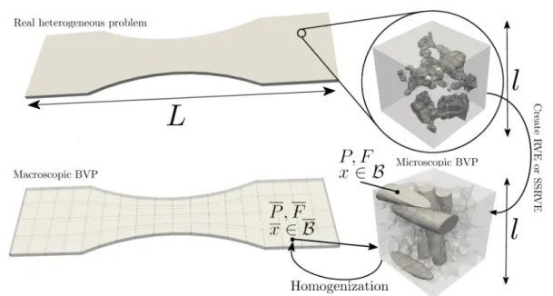
Throughout this paper, we will mark macroscopic quantities with bars, as, e.g., the deformation gradi- ent F and the first Piola-Kirchhoff stress tensor P . On the microscale, we use P for the stress and F for the deformation gradient. We do not have a phenomenolog- ical material law on the macroscale, instead, the macro- scopic quantities are assumed to be volumetric averages of quantities on the microscale. In Fig. 1, a schematic il- lustration of the homogenization approach FE

is given.

Let us remark that in recent years an approach to reduce the computational effort of an FE

simulation was to use RVEs with simplified geometries, e.g., con- sisting of ellipsoids; see [56, 55]. These statistically sim- ilar RVEs (SSRVEs) can be discretized with a coarser mesh. In Fig. 1, we depict a typical RVE (top right) as well as a typical SSRVE (bottom right).

2.1.1 Microscopic boundary value problems

We first introduce the microscopic boundary value prob- lem defined on a reference configuration B

, which rep- resents our microscopic RVE, using the corresponding reference variables X . Let us assume that in a deformed state B, the deformation of our reference configuration can be described by ϕ : B

→ B and the deformation gradient is defined by F := ∇ϕ. Then, without any further external forces, the balance of momentum in a weak formulation with a test function δx writes

−

!

B0

δx · (Div

P (F )) dV = 0. (1) The tensor P (F) is the first Piola-Kirchhoff stress ten- sor and in contrast to the macroscale, the relation be- tween P and F has to be described by a phenomenolog- ical material law, which describes the considered mate- rial sufficiently.

In our numerical experiments, we consider dual-phase steels and use an implementation [42] of a J2-elasto- plasticity model in FEAP as a material law on the microscale. Work on crystal plasticity is in progress.

The parameter choices and different yield stresses for

the martensitic and ferritic phases can be found in [12,

Fig. 10]. The nonlinear equation (1) is then solved by

Newton’s method. More precisely, we typically apply

a Newton-Krylov-FETI-DP or Nonlinear-FETI-DP ap-

proach to (1); see Section 3 for details.

Fig. 1

Illustration of the FE

homogenization approach.

Realistic and heterogeneous macroscopic boundary value problem of length scale

.

Zoom into the microstructure of the material of length scale

; we have

. From the microstructure, an RVE or SSRVE can be constructed (see bottom right for SSRVE).

Macroscopic and simplified boundary value problem on the domain

with quantities

and

. The deformation gradient

induces the boundary conditions of the microscopic BVP on the right.

Microscopic boundary value problem on domain

, which can be an RVE or SSRVE.

As mentioned before, the boundary conditions on the microscale are induced from the macroscopic defor- mation gradient F at the corresponding Gauß integra- tion point. In the case of Dirichlet conditions, we simply enforce x := F X for each boundary node X ∈ ∂B

on the microscale. Here, X are the variables in the ref- erence configuration B

and x is the microscopic solu- tion, i.e., x describes the deformed configuration B. As many homogenization approaches do, the FE

method assumes that the material can be characterized suffi- ciently by a repetitive periodic RVE and therefore the use of periodic boundary conditions is more reasonable.

We first split the boundary ∂B into two parts

∂B = ∂B

∪ ∂B

.

For each node X

∈ ∂B

exists an associated X

∈

∂B

and both have opposing outer normal vectors.

With fluctuation fields ˜ w

= x − F X

and ˜ w

= x − F X

we enforce the periodic boundary condition

˜

w

= ˜ w

∀ pairs X

∈ ∂B

and X

∈ ∂B

. To obtain regular systems, we additionally enforce ˜ w

=

˜

w

= 0 in the eight corners of each RVE.

2.1.2 Homogenization and macroscopic boundary value problem

Similarly to the microscopic boundary value problems, we can formulate the macroscopic problem in a given

reference configuration B

and reference variables X . Again, the balance of momentum in the weak formula- tion with a test function δx writes

!

B0

δx · (Div

P(F ) − f ) dV = 0, (2) where f is a volume force. We here disregard surface forces for simplicity.

On the macroscale, we do not have a material law to deliver an explicit relation between the deformation gradient F and the stress tensor P. Instead, the first Piola-Kirchhoff stress tensor P at a macroscopic Gauß point is obtained by homogenization, i.e., as a volu- metric average over the Piola-Kirchhoff stresses P of the corresponding RVE. Therefore, we have

P := 1 V

!

B0

P (F ) dV, (3)

where V := |B

| is the volume of the corresponding RVE. With (3) and the fact that we consider nonlinear material laws on the microscale, also (2) is nonlinear in the desired solution F . Thus, also on the macroscale, a Newton approach is used to solve (2). Standard tech- niques for the globalization of Newton’s method can be applied. In our computations, load stepping (pseudo time stepping) is utilized as a homotopy method; see below.

Let us briefly derive the Newton iteration formu-

lated in the macroscopic displacement u, such that F =

∇ϕ = I + ∇u, where I is the identity and ϕ the macro- scopic deformation. We assume that we have an initial value u

. Given finite element shape functions N

T

and their derivatives B

, we can derive a nonlinear residual in the k-th iteration of Newton’s method on a certain finite element from (2):

r

"

u

# :=

!

T

B

P

"

I + u

#

− N

f dV.

Here, P

marks the discretized stress tensor on element T available in all Gauß points of the element. For the macroscopic tangent, we then have

dk

"

u

#

=

!

T

B

A

"

I + u

#

B

dV, (4) where A

is the discretized macroscopic tangent mod- ulus, which again writes

A := ∂P

∂F = ∂

∂F

$ 1 V

!

B0

P (F)dV

%

(5) and is thus defined in each Gauß point. Using stan- dard finite element routines to assemble the tangent DK &

u

'

from dk

&

u

'

and R &

u

'

from r

&

u

' , we obtain the Newton iteration

u

= u

− DK "

u

#

R "

u

#

. (6)

We now provide a brief description how to compute A . Let us therefore remark that F is constant on a single RVE. We assume a decomposition of the microscopic deformation gradient F =: F+ F ( on a single RVE into F and a fluctuating part F. Using the chain rule and (3), ( this immediately leads to

A := ∂P

∂F = ∂

∂F

$ 1 V

!

B0

P (F) dV

%

(7)

= 1 V

!

B0

∂P (F )

∂F : ∂F + F (

∂F dV (8)

= 1 V

!

B0

A dV + 1 V

!

B0

A : ∂ F (

∂F dV ; (9) see also [60, equation (89)]. The first term in the sum (9) is a volumetric average over the tangent modulus A of the microscopic problem.

We only have to compute P and A after Newton’s method has converged on the microscale. Therefore, we can assume an equilibrium state of the weak formu- lation in (1). Exploiting this fact and using the finite

element basis of the RVE, a reformulation of the dis- cretized tangent modulus A

was provided in [60, Sec- tion 3.2]:

A

:= 1 V

) *

T∈τ

!

T

A

dV +

− 1

V L

(DK)

L. (10) Here, τ is the finite element discretization of B

into finite elements and A

the discrete microscopic tangent modulus defined in the Gauß points of the finite ele- ments. Then,

1 V

) *

T∈τ

!

T

A

dV +

is simply the discrete representation of

,

B0

A dV in (9).

The second term in (10) 1

V L

(DK )

L (11)

is the discrete form of

,

B0

A :

dV exploiting the balance of momentum on the microscale; see [60] for the derivation. Here, the tangential matrix DK of the microscopic BVP is obtained from assembly of finite element matrices

k

:=

!

T

B

A

B

dV,

where T ∈ τ are finite elements and B

are the deriva- tives of the shape functions. The matrix L has to be assembled also from the element contributions

l

:=

!

T

A

B

dV.

Here, L has the dimension n × s, where n is the num- ber of degrees of freedom in the RVE and s = 4 in two dimensions and, respectively, s = 9 in three spatial dimensions.

Let us remark that DK is simply the tangent in the final Newton step on the RVE and thus the application (DK)

L can be interpreted as solving a linear sys- tem with s right hand sides. If a direct solver is used, a mode for multiple right hand sides can be used or s additional forward backward substitutions have to be performed. However, if using an iterative solver such as a Nonlinear- or Newton-Krylov-FETI-DP method, the iterative solver has to be called s times; of course, infor- mation reuse and recycling techniques can be applied to reduce computational cost for the later iteration phases;

see Section 4 for details.

We finally provide an algorithmic description of a

single load step in Fig. 2, where a Nonlinear- or Newton-

Krylov-FETI-DP type method is used to solve the mi-

croscopic RVEs. Let us remark that usually the desired

macroscopic deformation cannot be applied in a sin- gle step but has to be applied in several consecutive load steps. This often is denoted as pseudo time step- ping. The step shown in Fig. 2 has to be repeated for each load step with increasing load. It is possible to use the solution u

from the n-th load step plus additional Dirichlet boundary conditions as an initial value u

for the Newton iteration in the (n + 1)-th load step.

Alternatively, an extrapolation approach using several former solutions can be beneficial; see also Section 4.

Let us remark that we do not consider volume forces f in this paper but prescribe a fixed deformation as Dirichlet boundary conditions on parts of the bound- ary ∂B

⊂ ∂B

in incremental load steps.

2.2 Implementation remarks

Our C/C++ implementation, the FE2TI software, uses PETSc 3.5.2 [5] and MPI.

2.2.1 Solving the macro problem

In most of our numerical examples, the macroscopic problem is solved by a sparse direct solver, i.e., UMF- PACK or MUMPS, where this is still feasible. In this case, we solve the macroscopic problem redundantly on all MPI ranks. For large FE

simulations, the macro- scopic problem can also be solved in parallel. We can use a Krylov method combined with, e.g., an algebraic multigrid (BoomerAMG) approach from the hypre li- brary [29] as a preconditioner. Here, the Krylov sub- space method and the AMG preconditioner will run on small MPI communicators obtained by an MPI Comm - split, the macro problem is thus solved redundantly on the subcommunicators. A parallel domain decomposi- tion method could also be applied on the macroscale but this approach has not been utilized in this paper.

We often reuse the communicators created for the mi- croscopic solvers (see below for details), but for small RVEs an additional split into communicators of efficient size is also possible. The complete macroscopic solution is finally collected on all MPI ranks of the subcommu- nicator and thus all MPI ranks. Let us also remark that the assembly process of the macroscopic problem is also parallelized and, as should be expected, scales perfectly.

2.2.2 Solving the micro problems

For each Gauß point of the macroscopic problem and thus for each microscopic problem, we introduce a sep- arate MPI communicator. In our implementation, we use MPI Comm split to create subcommunicators of equal size. Inter-communicator communication is not

necessary during the microscopic solves and the aver- aging of the different microscopic quantities; see points 1 to 4 in Fig. 2. To solve the microscopic BVPs, we use a Nonlinear- or Newton-Krylov-FETI-DP method; see Section 3 for details.

In order to compute L

(DK )

L (see (10)), we solve s linear systems with DK as left hand side, i.e., we have nine right hand sides in 3D or four right hand sides in 2D. If an iterative solver is used, this can be an expensive step and, in extreme cases, in our numerical experiments, the computation of the consistent tangent moduli can take up more than 50% of the total time to solution. Approximating L

(DK)

L or even discard- ing the matrix L

(DK )

L completely can be feasible alternatives even though superlinear convergence may be lost for the macroscopic problem.

A discussion of different strategies is provided in Section 4. Finally, we use collective communication to provide A

and P

on all MPI-ranks in order to as- semble the linearized macroscopic problem (6). This is efficiently performed by first collecting and summing up all averaged values on the first rank of each micro- scopic subcommunicator and a consecutive collection step using only those first ranks. Thereby, we avoid global communication involving all MPI ranks but only communicate on independent subsets of MPI ranks at the same time.

3 Parallel domain decomposition solvers

We use iterative multilevel methods to solve our nonlin- ear solid mechanics problems on the RVEs, i.e., mostly parallel domain decomposition methods of the linear or nonlinear FETI-DP type or algebraic multigrid. Our implementations of nonlinear FETI-DP domain decom- position methods, developed within the SPPEXA EX- ASTEEL project, have scaled to the full 786 432 cores [36]

of the Mira BG/Q Supercomputer (Argonne National Laboratory, USA) for a heterogeneous nonlinear hy- perelasticity problem with 60 billion unknowns; also see [35], for details on the method and implementation.

In [35], also results for nonlinear domain decomposi- tion on the SuperMUC supercomputer (LRZ, Munich, Germany), the Vulcan supercomputer (Lawrence Liver- more National Laboratory, USA), and the JUQUEEN supercomputer (JSC, J¨ ulich, Germany) are included.

For robustness, especially for heterogeneous problems,

we usually apply sparse direct solvers, i.e., PARDISO [54],

UMFPACK [15], or MUMPS [2] as local subdomain

solvers. Here, to speed up the Krylov iteration phase,

accelerating the forward-backward substitution in the

sparse direct solver is of interest [65]. In our implemen-

Chooseinitial macroscopic deformationF which fulfils the boundary conditions Repeatuntil convergence (Newton iteration):

1. Apply boundary conditions to RVEbased on macroscopic deformation gradient; e.g. enforce x=F Xon the boundary of the microscopic problem∂Bin the case of Dirichlet constraints.

2. Solvemicroscopic nonlinear boundary value problem using Nonlinear-FETI-DP, Newton-Krylov- FETI-DP, or related methods.

3. Computeand return macroscopic stresses as volumetric average over microscopic stressesP^h:

P^h= 1 V

"

T∈τ

#

T

P^hdV.

4. Compute and return macroscopic tangent moduli as average over microscopic tangent moduli A^h:

A^h= 1 V

⎛

⎝"

T∈τ

#

T

A^hdV

⎞

⎠− 1

VL^T(DK)⁻¹L

5. Assembletangent matrix and right hand side of the linearized macroscopic boundary value prob- lem usingP^handA^h.

6. Solvelinearized macroscopic boundary value problem.

7. Updatemacroscopic deformation gradientF.

Fig. 2

Algorithmic description. Overlined letters denote macroscopic quantities. Blue parts are computations on the microscale and thus the MPI subcommunicators obtained by MPI Comm split. Red parts are macroscopic computations performed on all MPI ranks. Algorithmic description taken from [36].

tation it is also possible to use efficient preconditioners such as multigrid for the local problems in nonlinear do- main decomposition; see [37, 38]. Shared-memory par- allelization on the node is an option in our software if a shared-memory parallel subdomain solver (such as PARDISO or BoomerAMG) are used; see [39]. There, parallelization of the finite element assembly, combin- ing PETSc and OpenMP, and the solution of the subdo- main problems, using PARDISO, was performed. Good scalability using up to four OpenMP threads for each MPI rank on an Intel Ivy Bridge architecture was ob- served and incremental improvements were obtained us- ing up to ten threads.

For voxel meshes, see, e.g., Fig. 3 and Fig. 4, geomet- ric multigrid methods or Fast Fourier (FFT) transform based solvers would be efficient alternatives, since they can profit from the tensor structure of such meshes.

In [19], the authors compare an FFT-based solution method with standard Q1 finite elements for a crystal plasticity problem defined on an RVE. As the FFT- based method exploits the tensor structure of the prob- lem, the authors use structured meshes (voxel meshes) for, both, the FFT-based approach as well as for the Q1 finite element meshes. For the FEM problems, a com- mercial code was applied. The authors concluded that with respect to computational cost the FFT-based ap- proach can be computationally cheaper by one to two orders of magnitude. Indeed, FFT-based computational homogenization approaches have successfully been used by different authors in recent years; see, e.g., [62, 32, 58, 44, 57, 16] and references therein. The FFT approaches are valued for the high efficiency when applied to voxel-

based RVEs with millions of degrees of freedom, and because voxel meshes from EBSD measurements, as in Fig. 3, can directly be used without further processing.

In FFT homogenization, e.g., based on [51], the number of iterations will depend on the contrast; see, e.g., [32].

Note that the approach presented in this paper dif- fers from other approaches, including those using FFT solvers on the microscale. In order to obtain better ap- proximations on the microscale, especially for plastic- ity, we use second order (P2) finite elements instead of simple linear tets (P1) or trilinear hexahedral elements (Q1). We then use an approach (SSRVEs) to construct RVEs using simple geometries, e.g., ellipsoids. However, the advantages of SSRVEs can only be exploited fully when using unstructured meshes, and we therefore use unstructured tetrahedral meshes, well adapted to the geometry. Our parallel domain decomposition methods can cope with these unstructured meshes, and the num- ber of Krylov iterations will be only slightly higher. We also use direct sparse solvers on the subdomains for high robustness of the numerical methods and usually obtain quadratic convergence of the overall Newton scheme; cf.

Fig. 18. We will see in our numerical results that, for our SSRVEs, unstructured meshes are clearly favorable;

see Section 4.2. We will also see that the unstructured meshes can also be allowed to be significantly, i.e., more than an order of magnitude, smaller than the structured meshes. Using adaptive mesh refinement could further expand the advantage but this is out of the scope of this paper.

Recent versions of PETSc include an efficient im-

plementation of iterative substructuring methods [66].

However, we apply our own parallel implementation [35, 41] which is earlier and also includes our most recent versions of nonlinear domain decomposition methods [40].

Let us briefly describe the linear and nonlinear FETI- DP domain decomposition methods, which we will uti- lize to solve the RVE problems on the microscale. In our computational homogenization approach, the micro problems are usually more challenging than the macro problem as a result of the heterogeneities, which have to be homogenized.

3.1 Parallel linear and nonlinear domain decomposition of FETI-DP type

Given a nonoverlapping domain decomposition Ω

, . . . , Ω

of the computational domain Ω ⊂ R

, we introduce the (generally) nonlinear operators K

, . . . , K

, defined on the subdomains, and the corresponding right hand sides f

, . . . , f

. In nonlinear domain decomposition, we usually obtain the operators K

, . . . , K

from the minimization of a nonlinear (e.g., hyperelastic) energy on the subdomains; see [33, equation (2.4)]. In Newton- Krylov-DD methods, the operators K

, . . . , K

are lin- ear as the domain decomposition is performed after Newton linearization.

In our FE

simulations, the domain Ω will be an RVE B

and K

, . . . , K

as well as f

, . . . , f

are deter- mined by (1). We define the block vectors u = (u

, . . ., u

), K(u)

= [K

(u

)

. . . K

(u

)

]

, f

= [f

, . . . f

]

. Using finite element assembly in primal variables, we obtain the partially assembled nonlinear operator K, (

K( ( ( u) = R

K(R

u) ˜

and the corresponding right hand side ˜ f = R

f. As in linear FETI-DP methods, the global coupling by partial finite element assembly is introduced to make the local problems invertible and to obtain numerical scalability.

As a result, the Jacobian D K(˜ ( u) can be assumed to be invertible, while it still maintains a favorable, partially decoupled, structure, i.e.,

D K(˜ ( u) =

⎛

⎜ ⎜

⎜ ⎜

⎝

DK

(˜ u) D K (

(˜ u)

. .. .. .

DK

(˜ u) D K (

(˜ u) D K (

(˜ u) . . . D K (

(˜ u) D K (

(˜ u)

⎞

⎟ ⎟

⎟ ⎟

⎠ .

We now define nonlinear FETI-DP methods as iter- ative methods for the solution of the nonlinear system (see [33, 40])

A(˜ u, λ) :=

3 K(˜ ( u) + B

λ − f ˜ B u ˜

4

= 3 0

0 4

. (12)

Since the nonlinear problem K(˜ ( u) = ˜ f − B

λ can very efficiently be parallelized, such methods can be highly scalable and nonlinear problems with billions of degrees of freedom [35] can be solved in a few min- utes. As in standard, linear FETI-DP methods [64, 22, 21, 41] the linear constraint B u ˜ = 0 enforces the conti- nuity across the subdomain boundaries, using Lagrange multipliers λ. However, as opposed to linear FETI-DP methods, the continuity is only achieved at convergence of the Newton iteration; see [33] for details.

The (generally) nonlinear system (12) can be solved using different strategies; see [40]. These methods are all equivalent to the classical FETI-DP method if K is a linear operator.

For our problems on the RVEs, we can apply New- ton’s method directly to (12). This was denoted Nonlinear- FETI-DP-1 in [33]. We will either use a classical Newton- Krylov FETI-DP approach, i.e., the microscopic BVP is first linearized and the FETI-DP method is applied to the linearized system, or Nonlinear-FETI-DP-1 is used, i.e., Newton linearization is applied to (12), and the Newton correction 5

δ˜ u

; δλ

6

can be computed from

3 D K(˜ ( u

) B

B 0

4 3 δ˜ u

δλ

4

=

3 K(˜ ( u

) + B

λ

− f ˜ B u ˜

4 . (13) A reduction to the Lagrange multipliers leads to a linear system of the form

F δλ

= d, (14)

which is solved iteratively by a Krylov method, e.g., GMRES, throughout this paper, preconditioned by the standard FETI-DP Dirichlet preconditioner [64].

4 Numerical results

If not marked otherwise, we use a Newton-Krylov-FETI-

DP approach for the solution of the microscopic RVE

problems, i.e., we have used the most conservative choice

among our FETI-DP methods. We also present results

using Nonlinear-FETI-DP-1 on the Theta supercom-

puter later on. This is the most conservative choice

among the recent Nonlinear-FETI-DP and Nonlinear-

BDDC methods [35, 33, 40]. In our numerical experi-

ments, if not denoted otherwise, the macroscopic prob-

lem is discretized using piecewise linear triangular ele-

ments (P1) in 2D and piecewise trilinear or quadratic

brick elements (Q1 or Q2) in 3D. In all our experiments

we stop the macroscopic Newton iteration if the norm

of the update is smaller than 1e− 6. We use a tolerance

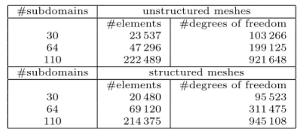
#subdomains unstructured meshes

#elements #degrees of freedom

30 23 537 103 266

64 47 296 199 125

110 222 489 921 648

#subdomains structured meshes

#elements #degrees of freedom

30 20 480 95 523

64 69 120 311 475

110 214 375 945 108

Table 1

Meshes for the SSRVEs. We use P2 finite elements.

of 1e − 8 for the microscopic Newton iteration and use a relative stopping tolerance of 1e − 9 for all Krylov subspace methods.

We use computing time on the JUQUEEN super- computer (J¨ ulich Supercomputing Centre), a large BG/Q (PowerBQC 16C 1.6 Ghz) installation with a total of 458 752 cores and 1 GB of memory for each core. JU- QUEEN was Europe’s fastest supercomputer in 2015 and is still ranked 22nd in the TOP500 list of Novem- ber 2017.

4.1 Simulation using a voxel-based RVE from EBSD measurements

In this section, we consider FE

simulations using a structured mesh based on voxel data obtained from EBSD (Electron Backscatter Diffraction) measurements as an RVE. We use P2 finite elements on the microscale, where each voxel is decomposed into six ten-noded tetra- hedra. The RVEs consisting of 663 552 finite elements and 2 738 019 degrees of freedom. Each RVE is decom- posed into 512 subdomains. We consider a plate with a hole discretized with 64 finite elements and thus using 512 RVEs. The sum of the number of degrees of free- dom on the microscale is thus approximately 1.4 billion.

We simulate four different deformations. We twist the plate and apply different pulling and pressing forces;

see Fig. 3 (top).

Each of the simulations has been performed using 262 144 MPI ranks using 131 072 cores of the JUQUEEN supercomputer. The numerical scheme remained stable and reliable results have been obtained; see Fig. 3. The I/O-time to write all data for all RVEs to the file system always stayed below 2% of the total runtime.

These results show the scalability of our implemen- tation and demonstrate its ability to run efficiently on large supercomputers, consistent with the earlier re- sults from [34, 36, 8]. Therefore, in the following sec- tions, we fokus on further optimizing and tailoring the RVE solver. We also investigate if we can reduce the size of the RVEs.

4.2 Considering different discretizations of the microscale

In this section, we study the influence of the structure and resolution of the discretization of a chosen RVE or SSRVE on the homogenized solution on the macroscale.

The construction of the SSRVEs using a fixed number of ellipsoidal inclusions based on EBSD measurements is discussed in [55]; also see [12]. Nonetheless, the resolu- tion of the discretization of the SSRVEs is comparably coarse in [55]. Here, we present a comparison of macro- scopic and microscopic results using meshes of differ- ent refinement levels; see Fig. 4 and Fig. 5 for different SSRVE meshes. We consider structured grids (Fig. 4), which cannot resolve the ellipsoidal inclusions very well, as well as unstructured grids (Fig. 5). These investiga- tions also provide us with a grid convergence study. As a macroscopic problem, we extend a symmetric plate discretized with 72 finite elements in x-direction; see Fig. 6 (left) for the undeformed geometry. We first ap- ply 11 load steps with a deformation of 0.025 percent of the current deformed state in each load step; see Fig. 6 (right) for a visualization of the load.

For our meshes, see Table 1. Our largest unstruc- tured mesh, discretizing the SSRVE using two ellip- soids [55], consists of 222 489 finite elements (see Fig. 5 right) and is chosen as our reference. When we to refer to the error (see Fig. 8), we mean the difference to the solution on the reference mesh.

In Fig. 7, we present the von Mises stresses in the macroscopic problem after 11 load steps using the ref- erence discretization. To compare the effects of using different SSRVE meshes on the macroscopic results, in Fig. 8, we depict the relative difference in the von Mises stresses between the reference solution from Fig. 7 and solutions obtained using coarser unstructured and struc- tured grids.

For the unstructured grids – see Fig. 8 (rows four to five) – we see only small differences for both grids and also observe convergence to the reference solution from the coarser grid (row four) to the finer one (row five).

On the other hand, we obtain significant differences us- ing structured grids, even though the finest structured SSRVE is of the same size as the unstructured refer- ence SSRVE; see Fig. 8 (rows one to three). Therefore, we can conclude that the choice of the discretization of the SSRVE has a significant impact. Our unstruc- tured grids result in a significant better approximation of the reference solution than all structured grids, even if the number of finite elements is an order of magnitude smaller.

All in all, in our experiments, the von Mises stresses

have been slightly higher when structured grids are

Fig. 3

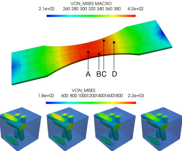
Four different types of macroscopic deformations. Simulations performed with RVEs with 663 552 finite elements and 2 738 019 degrees of freedom. The geometry of the RVEs corresponds to a small cubic part of a larger structure obtained from EBSD measurements of a dual-phase steel. The computations have been performed with 262 144 MPI ranks on 131 072 cores of JUQUEEN. Based on data from [12].

used. First, this is a result of high stress peaks caused by the unsmooth resolution of the surfaces of the el- lipsoids. Second, the minimal stresses in the SSRVEs appear to be slightly higher in the case of structured meshes. The first effect can be observed in the stress distributions in Fig. 9, where we depict the unstruc- tured SSRVE alongside the structured ones. In Fig. 9, four different Gauß points A,B,C, and D are considered as well as two different grid resolutions.

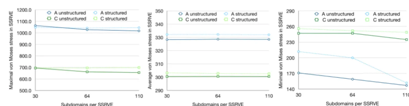
We additionally provide data on the stress peaks and the average stresses in Gauß points A and C in Fig. 10 (left and middle). The second effect is depicted in Fig. 10 (right) for the same two Gauß points A and C.

4.3 Improvements of the numerical scheme

In this section, we study techniques to improve the effi- ciency of our simulation. We also discuss the use of an approximate tangent in the solution of the macroscopic problem.

Our macroscopic test problem in this section con- sists of only 16 macroscopic finite elements, resulting in 128 microscopic RVE problems. Here, we always use the unstructured SSRVE with 47 296 finite elements de- composed into 64 FETI-DP subdomains; see Table 1.

In this section, a 1% deformation in x-direction using 21 load steps was applied on the macroscale; see also

Fig. 11 for the macroscopic solution. We keep the stop- ping criterion of the macroscopic and microscopic New- ton iterations fixed at 1e − 6 and, respectively, 1e − 8.

We keep the relative stopping criterion of the FETI-DP solver at 1e − 9 since the high accuracy is necessary for fast Newton convergence on the microscale.

We consider three improvements of our numerical scheme.

1. Lambda-recycling in FETI-DP: We reuse the so- lutions λ of earlier Newton steps as initial values for the FETI-DP solvers; see (14).

2. Approximate tangent modulus: We vary the stop- ping tolerance for the linear FETI-DP solves necessary for the computation of the consistent macroscopic tan- gent moduli; see (11). Stopping early leads to an ap- proximate tangent on the macroscale.

3. Extrapolation on the macroscale: We use an ex- trapolation approach to obtain a proper initial value for the Newton iteration on the macroscale.

Lambda-recycling In general, the idea of lambda-recycling in Newton-Krylov-FETI-DP is to use the solution λ

of the linear system from the k-th Newton iteration as an initial value for FETI-DP in the (k + 1)-th Newton iteration, e.g., to compute λ

.

We apply Newton-Krylov-FETI-DP on each RVE

in each macroscopic step and use lambda-recycling on

each RVE individually. Additionally, we use the solu-

Fig. 4

Structured discretization with similar numbers of finite elements as the unstructured in Fig. 5 and domain decompo- sition of an SSRVE with two ellipsoidal inclusions. The colors show the decomposition of the lower half of the cube and the ellipsoids.

20 480 finite elements and 30 subdomains.

69 120 finite elements and 64 subdomains.

214 375 finite elements and 110 subdomains.

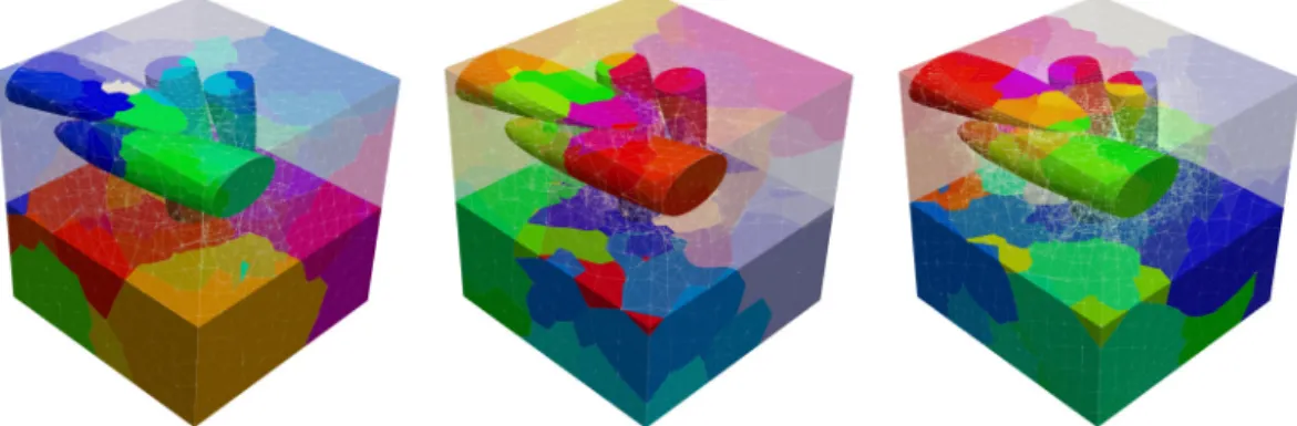
Fig. 5

Unstructured discretization and domain decomposition of an SSRVE with two ellipsoidal inclusions. The colors show the decomposition of the lower half of the cube and the ellipsoids.

23 537 finite elements and 30 subdomains.

47 296 finite elements and 64 subdomains.

222 489 finite elements and 110 subdomains.

Fig. 6

Macroscopic Problem.

undeformed Geometry;

scaled deformation (factor 50) after 10 steps.

Fig. 7

Von Mises stresses after 10 load steps using the largest of the three SSRVE.

tion from the last Newton-Krylov-FETI-DP iteration of the previous macroscopic step as an initial value for the first Newton-Krylov-FETI-DP iteration of the cur- rent macroscopic step. Let us remark that nonlinear FETI-DP methods do not need any lambda-recycling strategies since the reuse of information automatically arises from the nonlinear scheme.

It is interesting to note that when solving for the

nine right hand sides in (14), these right hand sides are

rather different and the lambda-recycling approach be-

tween those nine solves does not seem to be beneficial. It

turns out that it is more efficient to use lambda-recyling

from the nine individual solutions from the previous

macroscopic iteration. This strategy is thus standard

in our FE2TI software.

Fig. 8

Pointwise relative error in von Mises stresses on the macroscale using different SSRVEs after 7 (left column) and 11 load steps (right column). The reference solution is obtained using an SSRVE with a large unstructured mesh (see bottom right in Fig. 5). For the results in the first three rows, we use SSRVEs with structured meshes and for the last two rows SSRVEs with unstructured meshes -

SSRVE with structured mesh decomposed into 30 subdomains and 20 480 finite elements.

Second row:

SSRVE with structured mesh decomposed into 64 subdomains and 69 120 finite elements.

SSRVE with structured mesh decomposed into 110 subdomains and 214 375 finite elements.

SSRVE with unstructured mesh decomposed into 30 subdomains and 23 537 finite elements.

SSRVE with unstructured mesh decomposed into 64 subdomains and 47 296 finite elements.

Approximate tangent modulus The nine additional lin- ear FETI-DP solves to obtain a consistent tangent mod- ulus and thus a consistent tangent on the macroscale (see (14)) can exhibit a significant portion of the run- time, especially when using iterative solvers. Neverthe- less, it is necessary in order to obtain quadratic conver- gence of Newton’s method on the macroscale. We sug- gest to reduce the accuracy of the nine linear solves and thus use an approximate tangent on the macroscale. We therefore tested different stopping tolerances for FETI- DP for the computation of the consistent tangent mod- ulus.

Extrapolation of macroscopic solutions This approach is rather simple. If an extrapolation of the macroscopic iterates is activated in the FE2TI package, the initial

value for the (k+2)-th macroscopic load step u

is chosen as a linear extrapolation from the solutions of the k-th and (k + 1)-th load steps u

and, respec- tively, u

, i.e.,

u

= 2u

− u

.

4.4 Effects of the improvements

Without any of the improvements introduced in the

previous section, the FE

simulation takes 10 445.5s

to perform 21 macroscopic load steps using a total of

82 macroscopic Newton steps. Using lambda-recycling

alone, the runtime can be reduced to 7 693.0s, which is

1.36 times faster.

Fig. 9 From left to right:

von Mises stresses in four Gauß points A,B,C, and D after 10 load steps - the locations of the

points A to D is depicted above. The deformation of the SSRVEs is scaled by a factor of 20.

coarse

structured and unstructured discretizations with 20 480 and, respectively, 23 537 finite elements, both decomposed into 30

irregular subdomains.

fine structured and unstructured discretizations with 214 375 and, respectively,

222 489 finite elements, both decomposed into 110 irregular subdomains.

Fig. 10

Maximal stress

after 10 load steps in structured and unstructured SSRVEs attached to Gauß points A and C - see Fig. 9 for location of Gauß points; see Table 1 for the number of finite elements.

Fig. 11

Macroscopic solution of a small model problem after 17 load steps.

Choosing different accuracies for the computation of the consistent tangent modulus (1e − 9, 1e − 6, 1e − 3, 1e − 1), quadratic convergence of the macroscopic Newton iterations was lost only for 1e − 1, where the total number of Newton iterations in 21 load steps in- creases slightly from 82 to 88; see also Table 2.

The runtime is reduced from 7 693.0s to 5 573.5s for the tolerance 1e − 3, which is our best choice and cor- responds to a factor of 1.38 of reduction in runtime.

In Fig. 12, we provide a comparison of three vari- ants, namely without lambda-recycling and with lambda- recycling and different tolerances 1e − 9 and 1e − 3 for the consistent tangent.

Finally, adding the macroscopic extrapolation of so- lutions, the number of macroscopic Newton iterations is further reduced to 66, and thus also the runtime is reduced to 4 721.0s; see Table 2. Combining all three improvements, we can accelerate the computations by a factor of 2.2.

4.5 Large run using the improvements

Combining our different strategies, i.e., λ-recycling, ap- proximation of the consistent tangent moduli, and ex- trapolation of macroscopic solutions, we are able to sim-

Fig. 12

Runtime of the macroscopic Newton iterations.

Comparison between our software FE2TI without optimiza- tion, with lambda-recycling, and with lambda-recycling plus using an approximate tangent modulus with tolerance 1

3.

Additionally, the macroscopic load steps are marked in red on the x-axis.

ulate 81 load steps with a 2.1% total deformation in 4 hours and 39 minutes using 18 432 JUQUEEN cores.

Here, we use the unstructured SSRVE with 47 296 fi- nite elements, since the approximation of the reference solution showed to be accurate enough. We depict the final state of the solution in Fig. 13.

4.6 Improving scalability by exploiting parallelism on the macroscale

As mentioned above, the capability to solve the macro- scopic problem in parallel with an iterative Krylov sub- space method (e.g., CG or GMRES) and, e.g., the Boo- merAMG preconditioner [29] was included. When us- ing BoomerAMG, we always use HMIS coarsening, long range ext+i interpolation, and a nodal coarsening ap- proach; see [4] for a discussion of efficient parameters for elasticity.

The macroscopic problem is assembled and solved in

parallel on a subset of ranks of the MPI communicators

which are assigned to the RVEs. In our tests, these com-

municators have a reasonable size, e.g., 64 MPI ranks

if the RVE is decomposed into 64 subdomains. In the

following tests, we always use between 2 and 64 MPI

load lambda stopping tol. Newton It. Total steps recycling consistent tangent extrapolation Macroscale Runtime

21 no 1e-9 no 82 10 445.5s

21 yes 1e-9 no 82 7 693.0s

21 yes 1e-6 no 82 6 484.2s

21 yes 1e-3 no 82 5 573.5s

21 yes 1e-1 no 88 5 688.5s

21 yes 1e-3 yes 66 4 721.0s

Table 2

Improvements using lambda-recycling, inexact macroscopic Newton’s method, and extrapolation of the macroscopic problem.

Fig. 13

Von Mises stresses after 81 load steps and a total deformation of approximately 2.1% of the macroscopic reference configuration. Four SSRVEs A,B,C, and D (from left to right) are depicted.

ranks and thus AMG is only applied on a small num- ber of ranks. The result of the macroscopic problem is distributed to the complete communicator and then available on all MPI ranks. We perform two different weak scaling tests using the unstructured SSRVE with 64 subdomains and the best parameter settings found before, i.e., λ-recycling, approximation of the consis- tent tangent moduli, and extrapolation of macroscopic solutions are used.

We perform 13 load steps for an uniaxial tension test of a macroscopic cube. In the first weak scaling test, we use four MPI ranks for each JUQUEEN core and use up to 1.04 million MPI ranks; see Fig. 14 (top left and top

right) and Fig. 15 for the results. The results in Fig. 15 show significant improvements using parallelization of the macro problem.

In the second test, we use two MPI ranks per core and scale up to the complete machine; see Fig. 14 (bottom left and bottom right). Considering the av- erage time per macroscopic Newton iteration, we ob- tain an excellent efficiency of 74% on 1.04 million MPI ranks using AMG for the macroscopic problem and, re- spectively, for the setup using two MPI ranks per com- pute core, 78% parallel efficiency on the whole machine.

In both cases the scalability is increased drastically in

comparison to the approach using a direct solver on the macroscale.

4.7 Production runs on Theta using Nonlinear-FETI-DP-1

In this section, we present some results for large pro- duction runs using Nonlinear-FETI-DP-1 to solve the microscopic problems.

Theta is a large Intel Xeon Phi (Xeon Phi 7230, 64 Cores, 1.3 Ghz, “Knights Landing”) x86 installation at Argonne Leadership Computing Facility (ALCF) with a total of 231 424 cores and ranked 18th in the TOP500 list of November 2017. Theta is a very capable su- percomputer. Unfortunately, Intel has discontinued its Xeon Phi line and Theta’s successor named Aurora, planned to be the first exascale system of the USA in 2021, will use a different architecture.

Analogously to the last subsection, we use the ex- trapolation approach and an approximate consistent tangent. With Nonlinear-FETIDP-1, λ-recycling is not necessary. Indeed, the most conservative nonlinear FETI- DP method – Nonlinear-FETI-DP-1 – shows to be as robust and efficient as Newton-Krylov-FETI-DP with λ-recycling.

4.8 First run on Theta

We are able to simulate 171 load steps with a total deformation of 4.3% in exactly 4 hours walltime us- ing 36 864 cores of Theta (Argonne National Labora- tory, USA). Here, we use the unstructured SSRVE with 47 296 finite elements (see Table 1) since the approxi- mation of the reference solution showed to be accurate enough. The problem has 302 million degrees of free- dom in the microscale and 570 degrees of freedom on the macroscale

We depict the final state of the solution in Fig. 16 and the development of the von Mises stresses over time in Fig. 17 for six different vertices.

We also show the number of necessary Newton and FETI-DP iterations on the microscale. In Fig. 18 the effect of plastification of certain RVEs can be observed nicely by observing the number of Nonlinear-FETI-DP- 1 and GMRES iterations in different load steps. Clearly, starting at load step number four, RVEs A and B need more Newton steps to converge than C and D, which marks the point in time when these two RVEs start to show a plastic behavior.

This introduces a certain load imbalance and can also be observed in the corresponding runtimes; see

Fig. 19. This load imbalance shows to be of minor inter- est and does not affect the performance severly, since, after approximately 20 load steps, all RVEs in the crit- ical region show a plastic behavior and the load imbal- ance vanishes. To illustrate this effect, we also present the Newton iterations and Nonlinear-FETI-DP-1 run- times of load steps 70 to 79; see Fig. 18 (right) and Fig. 19 (right). We also present the number of GMRES iterations per Nonlinear-FETI-DP-1 solve in Fig. 20.

The average number of GMRES iterations per linear solve is approximately 40 for each of the four RVEs, which is a satisfactory result.

4.9 Second run on Theta

We finally present results for a refined macroscopic mesh with 1 792 SSRVEs computed on Theta using Nonlinear- FETI-DP-1. We simulate 319 load steps using 114 688 cores of Theta and obtain a deformation of 7.7% in x- direction. The problem has 693 million degrees of free- dom in the microscale and 1 305 degrees of freedom on the macroscale. Some results for different RVEs and different load steps are presented in Fig. 21.

4.10 Conclusion

We have presented a framework for parallel computa- tional homogenization using the FE

approach. The us- age of parallel domain decomposition solvers on the microscale and parallel algebraic multigrid solvers on the macroscale allows large multiscale simulations for micro-heterogeneous media. We have shown FE

simu- lations with million-way parallelism and billions of de- grees of freedom. Larger simulations will be possible once exascale supercomputers will become available.

AcknowledgmentsThe authors gratefully acknowledge the Gauss Centre for Supercomputing e.V. (www.gauss-centre.eu) for provid- ing computing time on the GCS Supercomputer SuperMUC at Leib- niz Supercomputing Centre (LRZ, www.lrz.de) andJUQUEEN[63]

at J¨ulich Supercomputing Centre (JSC, www.fz-juelich.de/ias/jsc).

GCS is the alliance of the three national supercomputing centres HLRS (Universit¨at Stuttgart), JSC (Forschungszentrum J¨ulich), and LRZ (Bayerische Akademie der Wissenschaften), funded by the Ger- man Federal Ministry of Education and Research (BMBF) and the German State Ministries for Research of Baden-W¨urttemberg (MWK), Bayern (StMWFK) and Nordrhein-Westfalen (MKW). This research used resources (Theta) of the Argonne Leadership Computing Facil- ity, which is a DOE Office of Science User Facility supported under Contract DE-AC02-06CH11357. The authors acknowledge the use of data from [12] provided through a collaboration in the DFG SPPEXA projectEXASTEEL.

The authors would also like to thank J¨org Schr¨oder, Dominik Brands, and Lisa Scheunemann(University of Duisburg-Essen) for providing the SSRVEs, the J2 plasticity model, and many fruitful discussions.

Fig. 14 Top Left:

Average Time for each macroscopic Newton iteration scaling to 1.02 million MPI ranks on JUQUEEN using CG plus AMG preconditioner or a direct solver, respectively.

Corresponding efficiency to runtimes presented in top left figure.

Average Time for each macroscopic Newton iteration scaling up to the complete JUQUEEN.

Bottom Right:

Corresponding efficiency to runtimes presented in bottom left figure.

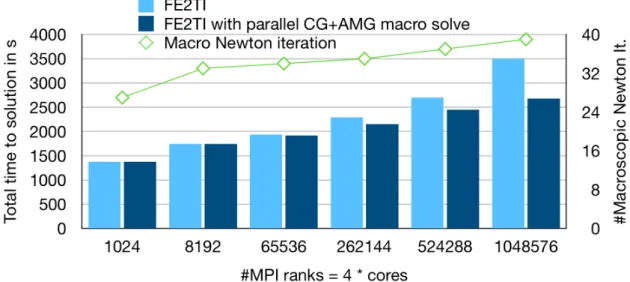
Fig. 15

Weak parallel scalability on JUQUEEN. Total time to solution of our FE

implementation FE2TI for 13 load steps using CG with an AMG preconditioner or, respectively, a direct solver on the macroscale. The largest problem has 3.3 billion degrees of freedom on the microscale and 7.8 thousand degrees of freedom on the macroscale.

References

1. Assyr Abdulle, Weinan E, Bj¨ orn Engquist, and Eric Vanden-Eijnden. The heterogeneous multiscale method.

Acta Numer., 21:1–87, 2012.

2. Patrick R. Amestoy, Iain S. Duff, Jean-Yves L’Excellent, and Jacko Koster. A fully asynchronous multifrontal solver using distributed dynamic scheduling. SIAM Jour- nal on Matrix Analysis and Applications, 23(1):15–41, 2001.

3. Allison H. Baker, Robert D. Falgout, Tzanio V. Kolev, and Ulrike Meier Yang. Scaling hypre’s multigrid solvers to 100,000 cores. In Michael W. Berry, Kyle A. Gal- livan, Efstratios Gallopoulos, Ananth Grama, Bernard Philippe, Yousef Saad, and Faisal Saied, editors, High- Performance Scientific Computing: Algorithms and Ap- plications, pages 261–279. Springer London, London, 2012.

4. Allison H. Baker, Axel Klawonn, Tzanio Kolev, Mar- tin Lanser, Oliver Rheinbach, and Ulrike Meier Yang.

Scalability of classical algebraic multigrid for elastic-

Fig. 16

Von Mises stresses after 171 load steps and a total deformation of approximately 4.3% of the macroscopic reference configuration. Four exemplary SSRVEs A,B,C, and D (from left to right) are depicted.

Fig. 17

Von Mises stress in six vertices of the macroscopic problem over pseudo time.

ity to half a million parallel tasks. In Hans-Joachim Bungartz, Philipp Neumann, and E. Wolfgang Nagel, editors, Software for Exascale Computing - SPPEXA 2013-2015, pages 113–140, 2016. vol. 113 of Springer Lect. Notes Comput. Sci. and Engrg. Also TUBAF Preprint 2015-14 at

forschung/preprints.

5. Satish Balay, Shrirang Abhyankar, Mark F. Adams, Jed Brown, Peter Brune, Kris Buschelman, Victor Eijkhout, William D. Gropp, Dinesh Kaushik, Matthew G. Knep- ley, Lois Curfman McInnes, Karl Rupp, Barry F. Smith, and Hong Zhang. PETSc users manual. Technical Report

ANL-95/11 - Revision 3.5, Argonne National Laboratory, 2014.

6. D. Balzani, D. Brands, and J. Schr¨ oder. Construction of statistically similar representative volume elements. In J. Schr¨ oder and K. Hackl, editors, Plasticity and beyond:

Microstructures, Crystal-Plasticity and Phase Transi- tions. CISM Lecture Notes No. 550, 2013.

7. D. Balzani, L. Scheunemann, D. Brands, and J. Schr¨ oder.

Construction of two- and three-dimensional statistically similar RVEs for coupled micro-macro simulations. Com- putational Mechanics, 54:1269–1284, 2014.

8. Daniel Balzani, Ashutosh Gandhi, Axel Klawonn, Martin Lanser, Oliver Rheinbach, and J¨ org Schr¨ oder. One-Way and Fully-Coupled FE

Methods for Heterogeneous Elas- ticity and Plasticity Problems: Parallel Scalability and an Application to Thermo-Elastoplasticity of Dual-Phase Steels, pages 91–112. Springer International Publish- ing, Cham, 2016. Also TUBAF Preprint: 2015-13,

//tu-freiberg.de/fakult1/forschung/preprints.

9. J.E. Bishop, J.M. Emery, R.V. Field, C.R. Weinberger, and D.J. Littlewood. Direct numerical simulations in solid mechanics for understanding the macroscale effects of microscale material variability. Comput. Meth. Appl.

Mech. Engrg., 287:262–289, 2015.

10. Joseph E. Bishop, John M. Emery, Corbett C. Battaile,

David J. Littlewood, and Andrew J. Baines. Direct nu-

merical simulations in solid mechanics for quantifying the

macroscale effects of microstructure and material model-

form error. JOM, 68(5):1427–1445, May 2016.

Fig. 18

Newton iterations on the microscale for the four RVEs A, B, C, and D (see Fig. 13 for position of RVEs); each block of four columns represents a single macroscopic Newton step in a certain macroscopic load step (marked on the x-axis).

Load steps 1 to 10.

Load steps 70 to 79.

Fig. 19

Runtime of Nonlinear-FETI-DP-1 on the microscale for the four RVEs A, B, C, and D (see Fig. 13 for position of RVEs); each block of four columns represents a single macroscopic Newton step in a certain macroscopic load step (marked on the x-axis).

Load steps 1 to 10.

Load steps 70 to 79.

Fig. 20

GMRES iterations per Nonlinear-FETI-DP-1 solve on the microscale for the four RVEs A, B, C, and D (see Fig. 13 for position of RVEs); each block of four columns represents a single macroscopic Newton step in a certain macroscopic load step (marked on the x-axis).

Load steps 1 to 10.

Load steps 70 to 79.

11. Felipe Bordeu, Pierre-Alain Boucard, and Pierre Gosse- let. Balancing domain decomposition with nonlinear re- localization: Parallel implementation for laminates. In P. Ivnyi B.H.V. Topping, editor, Proc. 1st Int. Conf. on Parallel, Distributed and Grid Computing for Engineer- ing, Stirlingshire, UK, 2009. Civil-Comp Press.

12. D. Brands, D. Balzani, L. Scheunemann, J. Schr¨ oder, H. Richter, and D. Raabe. Computational model- ing of dual-phase steels based on representative three- dimensional microstructures obtained from EBSD data.

Arch. Appl. Mech., 86(3):575–598, 2016.

13. Xiao-Chuan Cai and David E. Keyes. Nonlinearly pre- conditioned inexact Newton algorithms. SIAM J. Sci.

Comput., 24(1):183–200 (electronic), 2002.

14. Xiao-Chuan Cai, David E. Keyes, and Leszek Marcinkowski. Non-linear additive Schwarz precondi- tioners and application in computational fluid dynamics.

Internat. J. Numer. Methods Fluids, 40(12):1463–1470, 2002.

15. Timothy A. Davis. A column pre-ordering strategy for the unsymmetric-pattern multifrontal method. ACM Transactions on Mathematical Software, 30(2):165–195, June 2004.

16. T.W.J. de Geus, J. Vondejc, J. Zeman, R.H.J. Peerlings, and M.G.D. Geers. Finite strain FFT-based non-linear solvers made simple. Computer Methods in Applied Me- chanics and Engineering, 318:412 – 430, 2017.

17. Weinan E and Bjorn Engquist. The heterogeneous multi- scale methods. Commun. Math. Sci., 1(1):87–132, 2003.

18. Bernhard Eidel and Andreas Fischer. The heterogeneous multiscale finite element method for the homogenization of linear elastic solids and a comparison with the fe2 method. Computer Methods in Applied Mechanics and Engineering, 329(Supplement C):332 – 368, 2018.

19. P. Eisenlohr, M. Diehl, R.A. Lebensohn, and F. Roters. A

spectral method solution to crystal elasto-viscoplasticity

at finite strains. International Journal of Plasticity,

46:37–53, 2013.