Technical Report Series Center for Data and Simulation Science

(1)

Technical Report Series

Center for Data and Simulation Science

Axel Klawonn, Martin Lanser, Oliver Rheinbach, Janine Weber

Preconditioning the coarse problem of BDDC methods - Three- level, algebraic multigrid, and vertex-based preconditioners

Technical Report ID: CDS-2019-14

Available at https://kups.ub.uni-koeln.de/id/eprint/9713

Submitted on June 18, 2019

(2)

METHODS - THREE-LEVEL, ALGEBRAIC MULTIGRID, AND VERTEX-BASED PRECONDITIONERS^˚

AXEL KLAWONN^{: ;}, MARTIN LANSER^{: ;}, OLIVER RHEINBACH^§, AND JANINE WEBER^:

June 17, 2019

Abstract. A fair comparison of three Balancing Domain Decomposition by Constraints (BDDC) methods with an approximate coarse space solver is attempted for the first time. The comparison is made for a BDDC method with an algebraic multigrid preconditioner for the coarse problem, a three-level BDDC method, and a BDDC method with a vertex-based coarse preconditioner which was recently introduced by Clark Dohrmann, Kendall Pierson, and Olof Widlund. For the first time, all methods are presented and discussed in a common framework. Condition number bounds are provided for all approaches. All methods are implemented in a common highly parallel scalable BDDC software package based on PETSc, to allow for a fair comparison. Numerical results showing the parallel scalability are presented for the equations of linear elasticity. For the first time, this includes parallel scalability tests for the vertex-based approximate BDDC method.

Key words. approximate BDDC, three-level BDDC, multilevel BDDC, vertex-based BDDC AMS subject classifications.

1. Introduction. During the last decade, approximate variants of the BDDC (Balancing Domain Decomposition by Constraints) and FETI-DP (Finite Element Tearing and Interconnecting - Dual-Primal) methods became popular for the solution of various linear and nonlinear partial di↵erential equations [19,8,24,23,1,16,18,13, 15,9]. These methods di↵er from their exact relatives by an approximate solution of components of the preconditioner, most notably the coarse problem. An approximate solution of the coarse problem can reduce the numerical robustness slightly, but can increase the scalability of the method significantly. While multilevel BDDC, see [24, 23, 20, 21] and, recently, [1], is constructed by applying exact BDDC recursively to the coarse problem, in other approximate BDDC variants cycles of AMG (algebraic multigrid) are applied to the coarse problem; see, e.g., [19, 8,14]. Recently, vertex- based coarse spaces of reduced size have been suggested to approximate the original coarse system [9].

In [14], we already considered, in a common framework, several linear and nonlinear BDDC variants using AMG-based approximations, following the BDDC formulation from [19] for linear problems. We also compared their performance using our ultra scalable PETSc-based [4,5,6] BDDC implementation, applying BoomerAMG [11] for all AMG solves. In the current paper, we continue these e↵orts and include the aforementioned vertex-based BDDC as well as three-level and multilevel BDDC in our framework as well as in our software package. In addition to a description of all

˚This work was supported in part by Deutsche Forschungsgemeinschaft (DFG) through the Pri- ority Programme 1648 ”Software for Exascale Computing” (SPPEXA) under grants KL 2094/4-2 and RH 122/3-2.

†Department of Mathematics and Computer Science, University of Cologne, Weyertal 86-90, 50931 K¨oln, Germany, axel.klawonn@uni-koeln.de, martin.lanser@uni-koeln.de, janine.weber@uni- koeln.de, url:http://www.numerik.uni-koeln.de

‡Center for Data and Simulation Science, University of Cologne, Germany, url:http://www.cds.

uni-koeln.de

§Fakultät für Mathematik und Informatik, Institut für Numerische Mathematik und Optimierung, Technische Universität Bergakademie Freiberg, 09596 Freiberg, Germany, oliver.rheinbach@math.tu-freiberg.de

1

(3)

methods and their condition number bounds, we also include a numerical and parallel comparison. To the best of our knowledge, a comparison between three-level BDDC and BDDC with AMG-based coarse approximations, using implementations based on the same building blocks, to allow for a fair comparison, has not been considered before. Also, for the first time, parallel scalability tests for the vertex-based BDDC method [9] are presented.

As a common baseline in all our comparisons, we include the approximate AMG- based preconditioner which performed best in [14]. This specific variant is also related, but not identical to three preconditioners suggested in [8]. This was already discussed in [14] in detail.

The remainder of this paper is organized as follows: In section2, we introduce the model problem, outline the domain decomposition approach, and present an exact BDDC preconditioner for the globally assembled system. In sections 3 and 4, we describe three di↵erent approximate BDDC preconditioners in a common framework. Namely, we consider an approximate BDDC preconditioner using AMG, a three-level BDDC method, and a vertex-based BDDC preconditioner using a Gauss- Seidel method. Section 5 gives the theory and the condition number bounds for all three aforementioned approximate BDDC preconditioners. In section6, we provide some details of our parallel implementation. In particular, we implemented all three approximate preconditioners with the same building blocks, which allows us to directly compare the methods with each other regarding their computing time and parallel scalability. Finally, in section7, we present comparing results in three spatial dimensions. For all our numerical tests, we consider linear elasticity problems.

2. Exact BDDC preconditioner and model problem.

2.1. Linear elasticity and finite elements. We consider an elastic domain

⌦ÄR³. We denote withu:⌦ÑR³the displacement of the domain, withf a given volume force, and withg a given surface force onto the domain, respectively. In particular, we assume that one part of the boundary of the domain,B⌦D, is clamped, i.e., has homogeneous Dirichlet boundary conditions, and that the rest,B⌦N :“ B⌦zB⌦D, is subject to the surface forceg, i.e., a natural boundary condition.

WithH¹p⌦q:“ pH¹p⌦qq³, the appropriate space for a variational formulation is the Sobolev space H¹₀p⌦,B⌦Dq :“ tv P H¹p⌦q : v “ 0 on B⌦Du. The problem of linear elasticity then consists in finding the displacementuPH¹₀p⌦,B⌦Dq, such that (2.1)

ª

⌦

Gpxq"puq:"pvqdx`

ª

⌦

Gpxq pxqdivudivvdx“ xF,vy,

for allvPH¹₀p⌦,B⌦Dqfor given material parametersGand and the right-hand side xF,vy “ª

⌦

f^Tvdx`ª

B⌦N

g^Tvd .

The material parameters G and depend on the Young modulus E ° 0 and the Poisson ratio ⌫ P p0,1{2q by G“E{p1`⌫qand “⌫{p1´2⌫q. Furthermore, the linearized strain tensor "“ p"ijqîj is defined by "ijpuq:“ ¹2p^B_Bûxⁱj `^B_Bûx^jiq, and we use the notation

"puq:"pvq:“ ÿ3 i,j“1

"ijpuq"ijpvq and p"puq,"pvqq^L2p⌦q:“

ª

⌦

"puq:"pvqdx.

(4)

The corresponding bilinear form associated with linear elasticity can then be written as

apu,vq “ pG"puq,"pvqq^L2p⌦q` pG divu,divvq^L2p⌦q.

We discretize our elliptic problem of linear elasticity by low order, conforming finite elements and thus obtain the linear system of equations

(2.2) Kgu“fg.

2.2. Exact BDDC preconditioner for the assembled system. The exact BDDC preconditioner formulation from [19] is applied directly to the system (2.2).

Given is a nonoverlapping domain decomposition⌦i, i“1, . . . , N,of⌦such that

⌦“îN

i“1⌦i. Each subdomain⌦i is a union of finite elements,Wi, i“1, . . . , N, are the local finite element spaces, and the product space is defined byW “W1ˆ¨ ¨ ¨ˆWN. The global finite element space V^h corresponds to the discretization of ⌦ and we assume to have an assembly operator R^T, where R^T : W ÑV^h. By discretization of the given partial di↵erential equation restricted to ⌦i, we obtain a set of local problems

Kiui“fi, i“1,¨ ¨ ¨ , N.

Defining the block operators

K“

¨

˚˝ K1

. ..

KN

˛

‹‚, f “

¨

˚˝ f1

... fN

˛

‹‚,

we can write Kg :“ R^TKR and fg :“ R^Tf. Finally, the interface between the subdomains is defined as :“îN

i“1B⌦izB⌦.

We use the index for degrees of freedom on and for the remaining degrees of freedom despite the Dirichlet boundaryB⌦D, we use the indexI. For the construction of a BDDC preconditioner directly applicable to the assembled linear systemKgu“ fg, the interface is split into primal (⇧) and the remaining dual ( ) degrees of freedom. Usually, vertices are chosen as primal variables and the coarse space is augmented by averages over edges and/or faces.

Let us introduce the space ÄW Ä W of functions, which are continuous in all primal variables, and the assembly operators Rq^T and Rr^T with Rq^T : W Ñ WÄ and Rr^T :WÄÑV^h. UsingR, we can form the partially assembled systemq

(2.3) Kr :“Rq^TKRq

and can also obtain the globally assembled finite element matrixKg fromKr by

(2.4) Kg“Rr^TKrR.r

We denote the interior and interface variables with the indicesIand , respectively.

Ordering the interior variables first and the interface variables last, we obtain

(2.5) Kr “

˜ KII Kr^T_I Kr I Kr

¸ .

(5)

The matrix KII is block-diagonal and applications of K_II^´¹ only require local solves on the interior parts of the subdomains and are thus easily parallelizable. We further introduce the union of subdomain interior (I) and dual ( ) interface degrees of freedom as an extra set of degrees of freedom denoted by the indexB. The index B thus leads to an alternative representation of the partially assembled systemKr as

(2.6) Kr “

˜KBB Kr_⇧B^T Kr⇧B Kr⇧⇧

¸ .

LikeKII, the matrixKBB is a block-diagonal matrix and applications ofK_BB^´¹ only require local solves.

Adding usual scalings, e.g.,⇢-scaling [17] or deluxe-scaling [7], to the prolongation operators and thus definingRrD :V^hÑÄW, we obtain the BDDC preconditioner for Kg by

(2.7) M_BDDC^´¹ :“´

Rr^T_D´HPD

¯Kr^´1´

RrD´P_D^TH^T¯

;

see [19]. Here, the operator H:WÄÑ V^h is the discrete harmonic extension to the interior of the subdomains given by

(2.8) H:“

ˆ 0 ´ pKIIq^´¹Kr^T_I

0 0

˙ .

Finally, letPD:WÄÑÄW be a scaled jump operator defined by (2.9) PD“I´ED:“I´RrRr^T_D.

The original definition often used in the literature isPD:“B_D^TB; see [22, Chapter 6]

and [19] for more details. There,B is the jump matrix used in FETI-type methods.

Please note that in the standard definition, the BDDC preconditioner is formulated for the reduced interface problem, i.e., as

(2.10) M_BDDC–^´¹ S :“Rr^T_D, Sr^´¹RrD, S .

Here, the prolongation operator RrD, is formed in the same way as RrD only restricted to the interface variables , andS andSr are the subdomain interface Schur complements of the matrices Kg and K, respectively.r Let us remark that the preconditioned system M_BDDC^´¹ Kg has, except for some eigenvalues equal to 1, the same spectrum as the standard BDDC preconditioner formulated on the Schur complement; see [19, Theorem 1]. Here, we provide a related but slightly more direct proof: We first explicitly write the BDDC preconditionerM_BDDC^´1 as

M_BDDC^´¹ :“´

Rr_D^T ´HPD

¯Kr^´¹´

RrD´P_D^TH^T¯

“

˜I K_II^´¹Kr^T_IpI´Rr Rr^T_D, q 0 Rr^T_D,

¸ Kr^´¹

ˆ I 0

pI´RrD, Rr^TqKr IK_II^´¹ RrD,

˙

“

˜I K_II^´¹Kr^T_IpI´ED, q 0 Rr^T_D,

¸ Kr^´¹

ˆ I 0

pI´E_D,^T qKr IK_II^´¹ RrD,

˙ .

(6)

Using the block factorization Kr^´¹“

ˆI ´K_II^´¹Kr^T_I

0 I

˙ ˆK_II^´¹ 0 0 Sr^´¹

˙ ˆ I 0

´Kr IK_II^´¹ I

˙ ,

by a direct computation we obtain the alternative representation M_BDDC^´1 “

˜K_II^´¹`K_II^´¹Kr^T_IED, Sr^´¹E_D,^T Kr IK_II^´¹ ´K_II^´¹Kr^T_IED, Sr^´¹RrD,

´Rr^T_D, Sr^´¹E^T_D, Kr IK_II^´¹ Rr_D,^T Sr^´¹RrD,

¸ .

The multiplicationM_BDDC^´1 Kg finally yields M_BDDC^´¹ Kg“

ˆI U

0 M_BDDC^´¹ _´ S

˙

with U “ K_II^´¹KI ´K_II^´¹K^T_IRr^T_D, Sr^´¹RrD, S , with ED, “ Rr Rr^T_D, , and using K I “Rr^TKr I. Here, M_BDDC^´1 _´ is the classical BDDC preconditioner for the Schur complement; see (2.10). The result then follows from the fact, that the eigenvalues of a block-triangular matrix equal the union of the set of eigenvalues of the diagonal blocks.

3. Approximate BDDC Preconditioners. All approximate BDDC methods considered in this paper are based on an approximate solution of the coarse problem of BDDC. To ensure a simple and fair comparison, all approximate preconditioners are implemented using the same software framework; see also [13,14].

By block factorization, we obtain (3.1) Kr^´1“

ˆ K_BB^´1 0

0 0

˙

`

ˆ ´K_BB^´¹Kr_⇧B^T I

˙Sr_⇧⇧^´¹´

´Kr⇧BK_BB^´¹ I ¯ , whereSr⇧⇧ is the Schur complement

Sr⇧⇧“Kr⇧⇧´Kr⇧BK_BB^´¹ Kr_⇧B^T .

Note thatSr⇧⇧ represents the BDDC coarse operator. ReplacingSr_⇧⇧^´¹ by an approxi- mationSp_⇧⇧^´¹ in (3.1), we obtain an approximation forKr^´1 by

(3.2) Kp^´¹“

ˆ K_BB^´¹ 0

0 0

˙

`

˙ Sp_⇧⇧^´¹´

´Kr⇧BK_BB^´¹ I ¯ . ReplacingKr^´¹in (2.7) byKp^´¹, we define an approximation to the BDDC preconditioner, i.e.,

(3.3) Mx^´¹:“´

Rr^T_D´HPD

¯Kp^´¹´

RrD´P_D^TH^T¯ .

For the remainder of the article, all approximate BDDC preconditioners are marked with a hat. In the following sections, we compare three di↵erent approaches to formSp_⇧⇧^´¹, e.g., for the approximation of the coarse solve:

a) using AMG (algebraic multigrid) denoted byMx_BDDC,AMG^´¹ ; b) using exact BDDC recursively denoted byMx_BDDC,3L^´¹

c) using an exact solution of a smaller vertex-based coarse space denoted by Mx_BDDC,VB^´¹ .

Let us remark thatMx_BDDC,AMG^´¹ was denotedMx₃^´¹ in [14].

(7)

4. Examples of approximate BDDC preconditioners. In this section, we give three examples of approximate BDDC preconditioners presented in the notation introduced in section 3. First, we consider an approximate BDDC preconditioner using AMG to precondition Sr⇧⇧, second, a three-level BDDC method using BDDC itself to precondition Sr⇧⇧, and third, a vertex-based BDDC preconditioner using a Jacobi/Gauss-Seidel method in combination with a vertex-based coarse space to preconditionSr⇧⇧.

4.1. BDDC Preconditioner with AMG coarse preconditioner. Let us denote the application of a fixed number of V-cycles of an AMG method to Sr⇧⇧ by M_AMG^´¹ . By choosing M_AMG^´¹ in (3.2) as an approximation of Sr⇧⇧, i.e., by choosing Sp_⇧⇧^´¹ :“M_AMG^´¹ , we obtain

(4.1) Kp_AMG^´¹ “

ˆ K_BB^´¹ 0

0 0

˙

`

˙

M_AMG^´¹ ´

´Kr⇧BK_BB^´¹ I ¯ . Again, by usingKp_AMG^´¹ as an approximation for Kr^´¹ in (3.3), we obtain the inexact reduced preconditionerMx_BDDC,AMG^´¹ .

4.2. A Three-level BDDC. Alternatively, if we construct an exact BDDC preconditionerSp^´_⇧⇧¹ for the Schur complement matrixSr⇧⇧, (3.3) will become a three- level BDDC preconditionerMx_BDDC,3L^´¹ . This approach is equivalent to the three-level preconditioner introduced in [23], but formulated for the original matrixKg. In [23], the BDDC formulation for the Schur complement system on the interface is used and applied recursively. Since we use the BDDC formulation for the complete system matrix Kg, we consequently apply this approach to form the third level. We thus follow Section2.2and mark all operators and spaces defined for the third level with bars, e.g., I are the interior variables on the third level, while I are those on the second level. In Section5, we derive the same condition number bound as in [24,23].

Let us now describe the application of BDDC toSr⇧⇧in some more details. The basic idea of the three-level BDDC preconditioner is to recursively introduce a further level of the decomposition of the domain⌦into N subregions⌦¹, ...,⌦^N. Each subregion comprises a given number of subdomains. All primal variables ⇧ on the subdomain level are then again partitioned into interior, primal, and dual variables, i.e., I,⇧, and , with respect to the subregions; see also Figure 1 for a possible se- lection in 2D. Now, in principle, the subdomains take over the role of finite elements on the third level and the subregions the role of the subdomains. The basis functions of the third level are the coarse basis functions of the second level, localized to the subregions.

We therefore first define the spaceV^h, which is spanned by all coarse basis functions of the second level and denote byWi, i“1, ..., Nthe spaces which are spanned by the restrictions of the coarse basis functions to the subregions ⌦ⁱ, i “ 1, ..., N.

The product spaceW is now defined asW “W1ˆ...ˆW_N.

Using local Schur complements S_⇧⇧^pⁱ^q “ K_⇧⇧^pⁱ^q ´K_⇧B^pⁱ^qK_BB^pⁱ^q´¹K_⇧B^pⁱ^q^T on the subdomains and the block matrixS⇧⇧“diagpS_⇧⇧^p¹^q, ..., S_⇧⇧^p^N^qq, we can redefine

Sr⇧⇧“ ÿN i“1

R^p_⇧ⁱ^q^TS_⇧⇧^pⁱ^qR^p_⇧ⁱ^q, where R^T “`

R^p¹^q^T, ..., R^p^N^q^T˘

and R^pⁱ^q “diag´

R^p_Bⁱ^q, R^p_⇧ⁱ^q¯

, i “1, ..., N. Now we

(8)

can perform this assembly process only on the subregions, i.e.,

(4.2) Sj “

Nj

ÿ

i“1

R^p_⇧ⁱ^q^TS_⇧⇧^pⁱ^qR^p_⇧ⁱ^q, @j “1, ..., N ,

where Nj is the number of subdomains belonging to subregion ⌦^j. Obviously, Sr⇧⇧

takes over the role of Kg on the third level, while Sj takes over the role of Ki. Consequently, defining a prolongationR:V^hÑW, we can also write

Sr⇧⇧“R^TS R, withS“diagpS1, ..., S_Nq.

Let us introduce the space ÄW Ä W of functions, which are continuous in all primal variables⇧on the third level, and the assembly operatorsRq

T

:W ÑWÄand Rr^T :WÄÑV^h. UsingR, we can form the partially assembled systemq

(4.3) Sr:“Rq^TSR.q

Adding scalings to the prolongations as before and thus definingRrD:V^h ÑÄW, we obtain the BDDC preconditioner for the third level by

(4.4) M^´_BDDC¹ :“

ˆRr^T_D´HPD

˙Sr^´¹´

RrD´P^T_DH^T¯ .

The operatorH:WÄ ÑV^h is the discrete harmonic extension to the interior of the subregions and writes

(4.5) H:“

˜

0 ´`

S_II˘´1rS^T_I

0 0

¸ ,

with the blocksS_II andSr _I of the partially assembled matrix

(4.6) Sr“

˜

S_II Sr

T

r I

S _I Sr

¸ ,

and the jump operator defined asPD:“I´RrRr^T_D.

Now, by choosingSp_⇧⇧^´¹ :“M^´_BDDC¹ as approximation forSr_⇧⇧^´¹ in (3.2), i.e., by (4.7) Kp_3L^´¹“

ˆ K_BB^´¹ 0

0 0

˙

`

˙

M^´_BDDC¹ ´

´Kr⇧BK_BB^´¹ I ¯ ,

we can define

(4.8) Mx_BDDC,3L^´¹ :“´

Rr_D^T ´HPD

¯Kp_3L^´¹´

RrD´P_D^TH^T¯ .

Instead of invertingrS directly, we again can use a block factorization (4.9) Sr^´

1“

ˆ S^´_BB¹ 0

0 0

˙

`

˜

´S^´_BB¹Sr

T

⇧B

I

¸ Tr^´

1

⇧⇧

´ ´Sr_⇧BS^´_BB¹ I

¯,

(9)

I

⌦, V^h

⌦1 ⌦2 ⌦5 ⌦6

⌦3 ⌦4 ⌦7 ⌦8

⌦9 ⌦10 ⌦13 ⌦14

⌦11 ⌦12 ⌦15 ⌦16

⌦

¹

⌦

²

⌦

³

⌦

⁴

Fig. 1. Example of a domain decomposition in 2D in 16 subdomains and 4 subregions recursively. We mark in blue the interface between subdomains and in red the interface between subregions. Primal nodes⇧w.r.t. the subregions are depicted as red circles, while primal nodes⇧ w.r.t. the subdomains are depicted as blue circles. Inner or dual nodes w.r.t the subregions, i.e.,I or, respectively, , are depicted as green triangles or, respectively, red squares.

where the primal Schur complement on subregion level is Tr_⇧⇧“Sr_⇧⇧´rS_⇧BS^´_BB¹Sr^T_⇧B.

Note that, following [19, Theorem 1], the preconditioned systemM^´_BDDC¹ Sr⇧⇧ on the subregion level has the same eigenvalues as Rr

T D, Tr^´

1Rr_D, Tr except for some eigenvalues equal to 1. Here, we have the Schur complement Tr of Sr⇧⇧ on the interface of the subregions, the primally assembled Schur complement Tr of Sr on the interface of the subregions, and the splittingRrD“diagpI_I Rr_D, q. Therefore, we can use the condition number estimations provided in [24,23] analogously in Section5.

4.3. Vertex-Based BDDC Preconditioner. We further describe the following vertex-based preconditioner for the coarse problem, as introduced by Dohrmann, Pierson, and Widlund [9], in our framework. We denote the respective vertex-based preconditioner withMx_BDDC,VB^´¹ . Here, the preconditioner for the coarse problem can be interpreted as a standard two-level additive or multiplicative Schwarz approach.

In particular, the direct solution of the coarse problemSr^´_⇧⇧¹ is replaced by a precon- ditionerM_VB^´¹ based on a smaller vertex-based coarse space.

It was shown early in the history of FETI-DP and BDDC, that vertex nodes alone as coarse nodes are often not sufficient to obtain robust algorithms [10, 17]. Thus, coarse degrees of freedom for BDDC or FETI-DP are often associated with average values over certain equivalence classes, i.e., edges and/or faces. The basic idea of the coarse component of the preconditionerM_VB^´1is to approximate the averages over edges or faces using adjacent vertex values.

We denote the vertex-based coarse space by WÄ and the original coarse space by WÄ⇧. Then, analogously to [9], we define : WÄ Ñ ÄW⇧ as the coarse interpolant between the coarse space based on vertices and the original coarse space based on certain equivalence classes. It is important that the coarse basis functions ofÄW , i.e., the columns of , build a partition of unity in the original coarse space WÄ⇧. This is, e.g., fulfilled for the following definition of suggested in [9]. Let us first assume

(10)

WÄ⇧ consists of edge constraints only. Then, each row of corresponds to a single edge constraint and has, in the case of an inner edge, two entries of 0.5 in the two columns corresponding to the two vertices located at the endpoints of the edge. All other entries of the row are zero. In case of an edge touching the Dirichlet boundary with one endpoint, the corresponding row has a single entry of 1 in the column corresponding to the vertex located at the other end of the edge. Analogously, a partition of unity can be formed for coarse spacesWÄ⇧ consisting of face constraints.

Again analogously to [9], we define Sr⇧⇧,r :“ ^TSr⇧⇧ as the reduced coarse matrix. Note that the number of rows and columns of Sr⇧⇧,r equals the number of vertices for scalar problems. The preconditioner M_VB^´1 for the coarse matrix Sr⇧⇧ is then given as

(4.10) M_VB^´¹ “ Sr_⇧⇧,r^´¹ ^T`GSpSr⇧⇧q,

where GS denotes the application of a Gauss-Seidel preconditioner. In particular, M_VB^´¹ is simply a Gauss-Seidel preconditioner with an additive coarse correction.

In [9], solely edge averages or solely face averages are used which are each reduced to vertex-based coarse spaces as described above. In general, also the combination of vertices, edge, and face averages as coarse components can be considered and can be reduced to a solely vertex-based coarse space.

Now we can define the vertex-based approximate BDDC preconditioner by choos- ingSp_⇧⇧^´1 :“M_VB^´1 as approximation forSr_⇧⇧^´1 in (3.2). Then, we obtain the approxima- tionKp_VB^´¹ ofKr^´¹ by

(4.11) Kp_VB^´¹ “

ˆ K_BB^´¹ 0

0 0

˙

`

˙ M_VB^´¹´

´Kr⇧BK_BB^´¹ I ¯ ,

and finally

(4.12) Mx_BDDC,VB^´¹ “´

Rr^T_D´HPD

¯Kp_VB^´¹´

RrD´P_D^TH^T¯

; using the notation from (3.3); see also [9].

5. Condition number bounds. First, we need to make two assumptions, which are equivalent to Assumptions 1 and 2 in [19].

Assumption1. For the averaging operatorED,2:“RrpRr^T_D´HPDqwe have

|ED,2|²_K_Ä§ pH, hq|w|²_K_Ä, @wPW ,Ä

with pH, hqbeing a function of the maximal mesh sizehand the maximal subdomain diameterH.

Under Assumption1, the condition number of the exactly preconditioned system is bounded by

(5.1) pM_BDDC^´¹ Kgq§ pH, hq;

see, e.g., Theorem 3 in [19]. For our homogeneous linear elasticity test case (see section6), if appropriate primal constraints, e.g., edge averages and vertex constraints, are chosen, we obtain the condition number bound with pH, hq “Cp1`logpH{hqq².

(11)

Assumption2. There are positive constants ˜c andC, which might depend onr h andH, such that

˜

cu^TKur §u^TKup §Cur ^TKu,r @uPW .Ä

Now, we can prove the following Theorem 5.1 for the preconditioned operator Mx^´1Kg. In the proof, we basically follow the arguments in the proof of Theorem 4 in [19], but here we use exact discrete harmonic extension operators, i.e., an exact ED,2.This is in contrast to Theorem 4 in [19], where inexact discrete harmonic exten- sions are used, which is not necessary in our case. Although large parts of the proof are identical, we include the complete line of arguments here for the convenience of the reader.

Theorem 5.1. Let Assumptions1and2hold. Then, the preconditioned operator Mx^´¹Kg is symmetric, positive definite with respect to the bilinear form h¨,¨iKg and we have

1

Crxu, uy^Kg §xMx^´¹Kgu, uy^Kg § pH, hq

˜

c xu, uy^Kg, @uPV^h. Therefore, we obtain the condition number boundpMx^´¹Kgq§ ^C˜c^r pH, hq.

Proof. LetuPV^hbe given. We define

(5.2) w“Kp^´¹pRrD´P_D^TH^TqKguPÄW and thus also have

Kwp “ pRrD´P_D^TH^TqKgu.

Using Rr^TRrD “ I, yields Rr^TP_D^T “ Rr^TpI ´RrDRr^Tq “ 0 and thus rangepP_D^Tq Ä nullpRr^Tq. Hence, we obtain

(5.3) xu, uyKg “u^TRr^TpRrD´P_D^TH^TqKgu“u^TRr^TKwp “ xw,Rur yxK.

Using the Cauchy-Schwarz inequality and Assumption2, we can further estimate xw,Rur yxK§xw, wy¹_K_x^{²xRu,r Rur y¹_K_x^{²^Asm.§ ²a

Crxw, wy¹_K_x^{²xRu,r Rur y¹_K_Ä^{²

p2.4q

“ a

Crxw, wy¹_K_x^{²xu, uy¹K^{g². (5.4)

Combining equations (5.3) and (5.4), we havexu, uy^K^g §Crxw, wyxK. Using (5.2) and (3.3), we can prove the lower bound.

1

Crxu, uy^K^g § xw, wyKx p5.2q

“ u^TKgpRr^T_D´HPDqKp^´¹KpKp^´¹pRrD´P_D^TH^TqKgqu

“ xu,pRr^T_D´HPDqKp^´¹pRrD´P_D^TH^TqKguy^Kg

p3.3q

“ xu,Mx^´¹Kguy^Kg

(5.5)

Let us now prove the upper bound using Assumption1, (5.2), and (3.3).

xMx^´¹Kgu,Mx^´¹Kguy^K^g “ xpRr^T_D´HPDqw,pRr^T_D´HPDqwy^K^g

“ xRrpRr^T_D´HPDqw,RrpRr^T_D´HPDqwyKÄ

“ xED,2w, ED,2wyKÄ“ |ED,2w|²ÄK Asm.1

§ pH, hq|w|²KÄ

(5.6)

(12)

Together with Assumption2, we obtain xMx^´¹Kgu,Mx^´¹Kguy^Kg

p5.6q

§ pH, hq|w|²_K_Ä^Asm.2§ 1

˜

c pH, hq|w|²_K_x

p5.5q

“ 1

˜

c pH, hqxu,Mx^´¹Kguy^Kg. (5.7)

Using a Cauchy-Schwarz inequality in combination with (5.7), we finally obtain xu,Mx^´¹Kguy^K^g § pH, hq

˜

c xu, uy^K^g. ˝

For the preconditioners considered here, we replace the inverse operator of the Schur complement in the primal variablesSr_⇧⇧^´¹ by an approximationSp_⇧⇧^´¹. Therefore, we have to show that Assumption2used in the proof of Theorem5.1is still relevant and holds under certain assumptions.

Assumption3. There are positive constants ˆc andC, which might depend onp h andH, such that

ˆ

cu˜^T_⇧Sr⇧⇧u˜⇧§˜u^T_⇧Sp⇧⇧u˜⇧§Cpu˜^T_⇧Sr⇧⇧u˜⇧, @u˜⇧PWÄ⇧.

We can now prove the following lemma.

Lemma 5.2. Let Assumption 3 hold and Kp^´¹ be defined as in equation (3.2).

Then, Assumption 2holds withc˜:“minpˆc,1qandCr:“maxpC,p 1q. Proof. We first splitKp^´¹“A1`A2 into its two additive parts

A1:“

ˆ K_BB^´¹ 0

0 0

˙

and

A2:“

˙ Sp_⇧⇧^´¹´

´Kr⇧BK_BB^´¹ I ¯ .

The multiplicationA1Kr yields (5.8) A1Kr “

ˆ K_BB^´¹ 0

0 0

˙ ˜ KBB Kr_⇧B^T Kr⇧B Kr⇧⇧

¸

“

ˆ I K_BB^´¹Kr_⇧B^T

0 0

˙ .

By a direct computation we obtain A2Kr “

˙Sp_⇧⇧^´¹´

´Kr⇧BK_BB^´¹ I ¯˜

KBB Kr_⇧B^T Kr⇧B Kr⇧⇧

¸

“

ˆ ´K_BB^´1Kr_⇧B^T I

˙Sp_⇧⇧^´¹´

0 Sr⇧⇧

¯

“

˙ ´

0 Sp_⇧⇧^´¹Sr⇧⇧

¯

“

˜ 0 ´K_BB^´¹Kr_⇧B^T Sp_⇧⇧^´¹Sr⇧⇧

0 Sp_⇧⇧^´¹Sr⇧⇧

¸ (5.9)

(13)

Adding (5.8) and (5.9), yields the final result Kp^´¹Kr “

ˆ I G

0 Sp_⇧⇧^´¹Sr⇧⇧

˙

withG“K_BB^´¹Kr_⇧B^T pI´Sp_⇧⇧^´¹Sr⇧⇧q. Therefore, besides of additional eigenvalues equal to 1, Kp^´¹Kr and Sp_⇧⇧^´1Sr⇧⇧ have the same spectrum, and we have minpKp^´¹Krq “ min´

minpSp^´1_⇧⇧Sr⇧⇧q,1¯

and maxpKp^´¹Krq “ max´

maxpSp_⇧⇧^´1Sr⇧⇧q,1¯

. Consequent- ly, Assumption2holds with ˜c:“minpˆc,1qandCr:“maxpC,p 1q. ˝

For the preconditionerMx_BDDC,AMG^´1 , we now getCp and ˆcdepending on the prop- erties of the AMG V-cycle used and therefore

(5.10) pMx_BDDC,AMG^´¹ Kgq§Cr

˜

c pH, hq “ maxpC,p 1q

minpˆc,1q pH, hq.

For the three-level BDDC preconditionerMx_BDDC,3L^´¹ we obtain, with Lemma 4.6 in [24] in two spatial dimensions and Lemma 4.7 in [23] in three spatial dimensions, ˆ

c“ ¹

C3L

´

1`logp^HH^ˆq¯2 andCp“1. Here, ˆHis the maximal diameter of a subregion and of course, depending on the problem and dimension, sufficient primal constraints on the second level have to be chosen; see [24,23]. Let us note that the results in [24,23] are only proven for scalar di↵usion problems. To the best of our knowledge an extension to linear elasticity has not been published so far and is still an open problem. Using Lemma5.2and Theorem 5.1, we obtain the condition number bound

(5.11) pMx_BDDC,3L^´¹ Kgq§ Cr

˜

c pH, hq “C3L

˜ 1`log

˜Hˆ H

¸¸2

pH, hq; see also [24,23].

For the vertex-based BDDC preconditionerMx_BDDC,VB^´¹ we obtain, with Theorem 3 in [9] for edge-based or face-based coarse spaces and quasi-monotone face-connected paths,pc• C¹1,maxpC,p 1q§CC and pH, hq “ C`

1`logp^Hhq˘2

; see [9, Theorem 3].

Here, CC is obtained by a coloring argument and therefore usually CC • 1. The constant C1 depends on geometric constants, e.g., the maximum number of subdomains connected by an edge (see [9, Lemma 2]), the maximum number of neighbors of a subdomain (see [9, (4.3)]), or typical subdomain sizes (see [9, Assumption 3]).

Additionally,C1depends on a tolerance for the lowest coefficient along an acceptable path; see [9, Assumption 1 and 2]; cf. also [12]. The results in [9] are proven for scalar di↵usion and linear elasticity problems. All together, with another constantCV B, we obtain

maxpC,p 1q

minpˆc,1q §CV B;

see also [9, Theorem 1 and 3] where pc“ ¹ andCp “ ² for the constants 1 and 2

used in [9]. Typically, we haveC1•1, and we then can defineCV B“C1¨CC. Using Theorem 1, we thus obtain the condition number bound

(5.12) pMx_BDDC,VB^´¹ Kgq§Cr

˜

c pH, hq§CV B pH, hq; see also [9, Theorem 3].

(14)

5.1. The GM (Global Matrix) Interpolation. Good constants ˜c,Cr in As- sumption2or, respectively, ˆc,Cpin Assumption3, are important for a small condition number and therefore a fast convergence of the approximate BDDC method. It is well known that for scalability of multigrid methods the preconditioner should preserve nullspace or near-nullspace vectors of the operator. Therefore, the AMG method should preserve the nullspace of the operator on all levels and these nullspace vectors have to be in the range of the AMG interpolation. While classical AMG guarantees this property only for constant vectors, the global matrix approach (GM), introduced in [3], allows the user to specify certain near-nullspace vectors, which are interpolated exactly from the coarsest to the finest level; details on the method and its scalability can be found in [3,2]. Since we are interested in linear elasticity problems, we choose the rotations of the body for the exact interpolation. All translations of the body are already interpolated exactly in classical AMG approaches for systems of PDEs since they use classical interpolation applied component-by-component. In Mx_BDDC,AMG^´¹ AMG is applied toSr⇧⇧and thus we need the three rotations in the spaceWÄ⇧, which is the restriction of WÄ to the primal constraints. Therefore, we first assemble the rotations of the subdomains ⌦i locally, extract the primal components, and finally insert them into three global vectors in WÄ⇧. In our implementation, we always use BoomerAMG from the hypre package [11], where a highly scalable implementation of the GM2 approach is integrated; see [2]. Let us remark that GM2 is one of two variants to choose the interpolation implemented in BoomerAMG and is recommended to use instead of GM1. In [2] it also showed a better scalability than GM1. We will compare the use of the GM2 approach with a hybrid AMG approach for systems of PDEs. By hybrid AMG approaches, we refer to methods, where the coarsening is based on the physical nodes (nodal coarsening) but the interpolation is based on the degrees of freedoms. In general, a nodal coarsening approach is beneficial for the solution of systems of PDEs, and all degrees of freedom belonging to the same physical node are either all coarse or fine on a certain level. The latter fact is also mandatory for the GM2 approach. Therefore, GM2 is based on the same nodal coarsening and can also be considered as a hybrid approach.

6. Implementation and Model Problems. Our parallel implementation uses C/C++ and PETSc version 3.9.2 [6]. All matrices are completely local to the computational cores. All assemblies and prolongations are performed using PETScVec- Scatter and VecGather operations. A more detailed description of the parallel data structures of our implementation of the linear BDDC preconditioner can be found in [14], where di↵erent nonlinear BDDC methods are applied to hyperelasticity and elasto-plasticity problems.

Since the preconditioners for the coarse problem are in the focus of this paper, we include some details on the implementation of the di↵erent variants. In general, the coarse problem Sr⇧⇧ is assembled on a subset of the available cores. The number of cores can be chosen arbitrarily and should depend on the size of the coarse problem to obtain a good performance. While BoomerAMG and BDDC itself can be applied to Sr⇧⇧ in parallel, for exact BDDC (M_BDDC^´¹ ) a sequential copy of Sr⇧⇧

is sent to each computational core and a sparse direct solver is applied. This is, of course, not scalable in parallel and one would prefer to avoid it. Using a sequential Gauss-Seidel implementation inMx_BDDC,VB^´¹ also requires a sequential copy ofSr⇧⇧and additionally sequential copies ofSr⇧⇧,r:“ ^TSr⇧⇧ , and eventually, depending on the implementation, also of . This can be avoided using a parallel implementation of

(15)

the Gauss-Seidel preconditioner. Therefore, as an alternative to the sequential approach, we also use the parallel PETSc implementation of SOR/Gauss-Seidel, which is in fact a block Jacobi preconditioner in between the local blocks associated with the di↵erent MPI ranks and an SOR/Gauss-Seidel preconditioner on the local blocks themselves. This can obviously deteriorate the convergence of the method, but we only have to build a local copy ofSr⇧⇧,r, which is much smaller compared toSr⇧⇧. All other matrices can be stored in a distributed fashion. Let us finally remark that we can apply the Gauss-Seidel preconditioner additively as described in(4.10)as well as multiplicatively, which is of course more robust.

7. Numerical Results. In this paper, we restrict ourselves to homogeneous linear elasticity problems. For heterogeneous examples or di↵erent model problems we refer to [14] forMx_BDDC,AMG^´¹ or [9] forMx_BDDC,VB^´¹ . All computations are performed on magnitUDE supercomputer (University of Duisburg-Essen) or JUWELS (FZ Juelich).

7.1. Three-Level BDDC and BDDC with AMG coarse preconditioner.

We first concentrate on a comparison between Mx_BDDC,3L^´¹ and Mx_BDDC,AMG^´¹ , which clearly have the largest parallel potential, especially due to the larger coarsening ratio from the second to the coarsest level. Also Mx_BDDC,3L^´¹ can be easily extended to a multilevel preconditioner while Mx_BDDC,AMG^´¹ already consists of several levels. The alternativeMx_BDDC,VB^´¹ is limited in scalability by construction, since the vertex-based coarse space is always solved by a sparse direct solver in our implementation. We therefore analyze and compareMx_BDDC,VB^´1 separately insubsection 7.2.

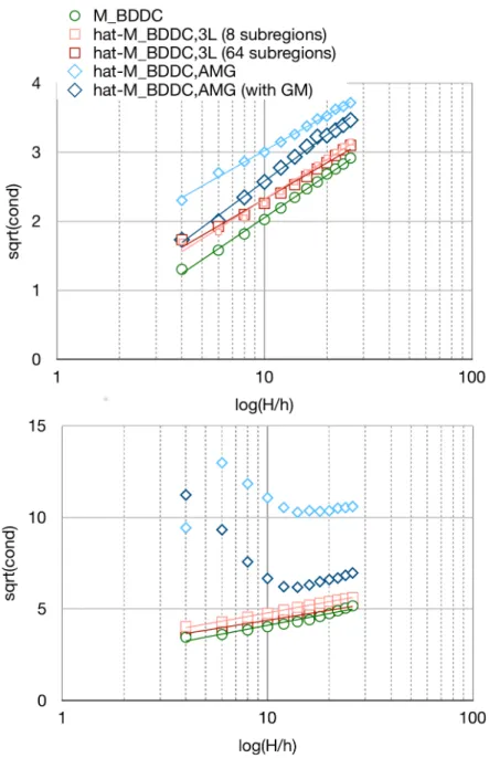
To have a theoretical baseline, we always include the exact BDDC preconditioner M_BDDC^´¹ in all figures. To verify the quadratic dependence of the condition number on the logarithm of H{h, which can be seen as a measure of the subdomain size, we provideFigure 2. There, we consider a linear elastic cube decomposed into 512 subdomains with Young modulusE“210GP aand di↵erent Poisson ratios. As a coarse space we enforce continuity in all vertices and in all edge averages. With a Poisson ratio of 0.3 (Figure 2(top)), all methods show a similar behavior and the condition numbers are comparable to the exact BDDC preconditioner. For Mx_BDDC,AMG^´¹ it is useful to include the GM approach, while for Mx_BDDC,3L^´¹ both tested setups, i.e., 8 or 64 subdomains per subregion, show a similar behavior. Choosing a larger Pois- son ratio of 0.49 ( Figure 2 (bottom)), Mx_BDDC,AMG^´¹ has higher condition numbers, especially for small subdomain sizes. But for larger subdomain sizes and using GM, Mx_BDDC,AMG^´¹ again shows a similar behavior. Let us remark that we always use a highly scalable AMG setup, i.e., aggressive HMIS coarsening, ext`i long range interpolation, nodal coarsening, a threshold of 0.3, and a maximum of three entries per row in the AMG interpolation matrices. Less aggressive strategies might show lower condition numbers, but we explicitly optimized the parameters to obtain good parallel scalability; see [2].

For the same setup with a Poisson ratio of 0.3 but fixedH{h“24, we perform a weak scaling study inFigure 3 up to 4096 cores. Considering the number of cg iterations until convergence (Figure 3(top)), the GM approach is necessary inMx_BDDC,AMG^´¹ to obtain results of similar quality as Mx_BDDC,3L^´¹ . The same can be observed considering the time to solution; seeFigure 3(bottom). The time to solution is always the complete runtime measured from the program start until it finishes. This especially includes the assembly of the linear system, the setup of the preconditioner, and the iteration/solution. Of course, the exact BDDC preconditioner does not scale due to

(16)

Fig. 2. Homogeneous linear elastic cube decomposed into 512 subdomains with H{h “ 4,6, ...,26. Top: E “ 210.0 and ⌫ “ 0.3; Bottom: E “ 210.0 and ⌫ “ 0.49. We vary the number of subdomains per subregion inMx_BDDC,3L^´1 and we compare nodal AMG and AMG-GM in Mx_BDDC,AMG^´1 . Computed on the magnitUDE supercomputer.

the sequential coarse solve.

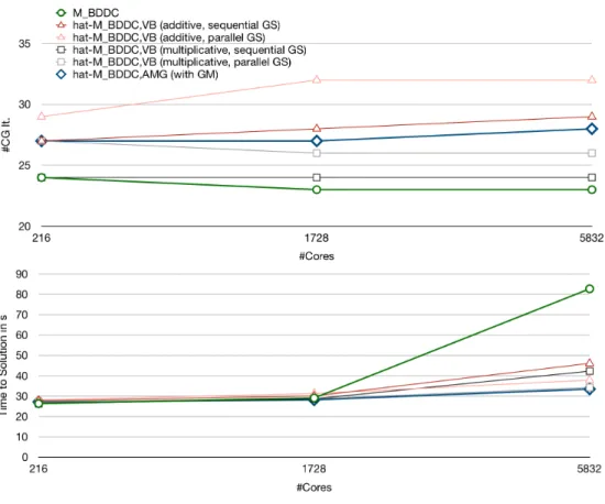
7.2. Vertex-Based BDDC. We provide a weak scaling test up to 5 832 cores forMx_BDDC,VB^´¹ for a similar model problem, i.e., linear elasticity with a Poisson ratio of 0.3 and a Young modulus of 210GP a. InFigure 4we provide a comparison with exact BDDC and Mx_BDDC,AMG^´¹ using GM with respect to cg iterations as well as

(17)

Fig. 3. Comparison ofM_BDDC^´1 ,Mx_BDDC,3L^´1 with 8 or 64 subregions, andMx_BDDC,AMG^´1 with and without GM. Using vertex and edge constraints. Homogeneous linear elastic cube decomposed into 64,512, and4 096subdomains withH{h“24. Top: Number of CG iterations;Bottom: Total time to solution including assembly of sti↵ness matrices, setup of the preconditioner and solution phase. Computed on JUWELS.

time to solution. Considering Mx_BDDC,VB^´¹ , a multiplicative combination of Gauss- Seidel applied to Sr⇧⇧ and the direct solve of the vertex based coarse problem is always the better choice compared to an additive variant. The parallel Gauss-Seidel method, which - as implemented in PETSc - is in fact a block Jacobi preconditioner in between the processors parts of the matrix, always results in more cg iterations but faster runtimes. With respect to parallel scalability, the best variant ofMx_BDDC,VB^´¹ is competitive with Mx_BDDC,AMG^´¹ , at least up to the moderate core count of 5 832. For an increasing number of cores, we expectMx_BDDC,AMG^´¹ to outperformMx_BDDC,VB^´¹ due to its inherent multilevel structure.

8. Conclusion. We have presented di↵erent approaches to approximate the coarse solve in BDDC and compared them with respect to theory and parallel scalability for the first time. If an appropriate AMG approach is available, e.g., the GM approach in the case of linear elasticity problems, Mx_BDDC,AMG^´¹ andMx_BDDC,3L^´¹ show a very similar behavior and both variants can be recommended. Up to a moderate number of compute cores alsoMx_BDDC,VB^´¹ can be an adequate alternative. An advan- tage ofMx_BDDC,VB^´¹ is the fact that neither a further decomposition into subregions is necessary nor an appropriate AMG method has to be chosen. On the other hand, the parallel potential of Mx_BDDC,VB^´¹ is limited, since it is not easily extendable to an arbitrary number of levels.

(18)

Fig. 4. Comparison of M_BDDC^´1 , Mx_BDDC,VB^´1 using additive/multiplicative sequential/parallel Gauss-Seidel, andMx_BDDC,AMG^´1 with GM. Using only edge constraints. Homogeneous linear elastic cube withH{h “22. Top: Number of CG iterations;Bottom: Total time to solution including assembly of sti↵ness matrices, setup of the preconditioner and solution phase. Computed on the magnitUDE supercomputer.

Acknowledgments. The authors gratefully acknowledge the computing time granted by the Center for Computational Sciences and Simulation (CCSS) of the Uni- versit¨at of Duisburg-Essen and provided on the supercomputer magnitUDE(DFG grants INST 20876/209-1 FUGG, INST 20876/243-1 FUGG) at the Zentrum f¨ur Informations- und Mediendienste (ZIM).

The authors gratefully acknowledge the Gauss Centre for Supercomputing e.V.

(www.gauss-centre.eu) for funding this project by providing computing time on the GCS SupercomputerJUWELSat J¨ulich Supercomputing Centre (JSC).

REFERENCES

[1] Santiago Badia, Alberto F. Mart´ın, and Javier Principe. Multilevel Balancing Domain Decom- position at Extreme Scales. SIAM J. Sci. Comput., 38(1):C22–C52, 2016.

[2] Allison H. Baker, Axel Klawonn, Tzanio Kolev, Martin Lanser, Oliver Rheinbach, and Ul- rike Meier Yang. Scalability of Classical Algebraic Multigrid for Elasticity to half a Million Parallel Tasks. In Software for Exascale Computing—SPPEXA 2013–2015, volume 113 of Lect. Notes Comput. Sci. Eng., pages 113–140. Springer, [Cham], 2016.

[3] Allison H. Baker, Tzanio. V. Kolev, and Ulrike M. Yang. Improving algebraic multigrid in-