Technical Report Series Center for Data and Simulation Science

(1)

Technical Report Series

Center for Data and Simulation Science

Alexander Heinlein, Christian Hochmuth, Axel Klawonn

Fully algebraic two-level overlapping Schwarz preconditioners for elasticity problems

Technical Report ID: CDS-2019-21

Available at https://kups.ub.uni-koeln.de/id/eprint/10441

Submitted on December 16, 2019

(2)

Fully algebraic two-level overlapping Schwarz preconditioners for elasticity problems

Alexander Heinlein

^1,2

, Christian Hochmuth

¹

, and Axel Klawonn

^1,2

1 Introduction

We consider the solution of large, parallel distributed stationary and dynamic dis- cretized elasticity problems with a moderate Poisson ratio; i.e., we do not consider the nearly incompressible case. As the solver, we use the Generalized Minimal Residual (GMRES) method preconditioned by two-level overlapping Schwarz precondition- ers with Generalized Dryja–Smith–Widlund (GDSW) [2, 3] and Reduced dimension GDSW (RGDSW) [5, 12] coarse spaces. Even though these preconditioners can be constructed from the fully assembled system matrix, a minimum of geometric in- formation is also needed. In particular, the domain decomposition interface and the null space are used for their construction. Here, we focus on the construction of fully algebraic GDSW type coarse spaces if this information is not available. In particular, we consider the case when the system matrix is uniquely distributed, such that the interface cannot be identified.

Therefore, we will describe a method to approximate the nonoverlapping subdo- mains, resulting in an approximate interface; cf. [10]. Our parallel implementation is based on the

FROSch

framework [9], which is part of the

ShyLU

package in Trilinos [13]; see [11, 10] for more details on the implementation. To discuss the performance of the fully algebraic approach, we will compare it to the classical GDSW type coarse spaces using all necessary information.

1Department of Mathematics and Computer Science, University of Cologne, Weyertal 86-90, 50931 Köln, Germany

2Center for Data and Simulation Science, University of Cologne, Germany, url:http://www.cds.uni-koeln.de

1

(3)

2 A. Heinlein, C.Hochmuth, A.Klawonn

2 Model Problems

The equilibrium equation for an elastic body covering the domain

Ω=[0,1]³

under the action of a body force

f

in the time interval

[0,T]

is

∂_ttu−

div

σ= f

in

Ω× [0,T],

(1)

with the symmetric Cauchy stress tensor

σ

and the displacement

u. We consider a

Saint Venant-Kirchhoff material, a hyperelastic material with the linear material law

σ(E)=λ

2

(

trace E)

²+µ

trace EI (2)

and the nonlinear strain tensor given by E :=

¹₂(C−I),

where C is the right Cauchy- Green tensor. Furthermore, we consider the boundary conditions

u

=

0 on

∂Ω_D

:=

{

0

} × [

0, 1

]², σ·

n

=

0 on

∂Ω_N

:=

∂Ω\∂Ω_D,

and the body force

f =(−20,

0, 0)

^T

, for

t<

5

·

10

⁻³

, and

f =

0, afterwards.

In addition to this, we also consider a stationary problem with

∂_ttu=

0, i.e., div

σ=(

0,

−

100, 0

)^T

in

Ω,

u

=

0 on

∂Ω_D

:=

{

0

} × [

0, 1

]², σ·

n

=

0 on

∂Ω_N

:=

∂Ω\∂Ω_D.

(3)

We transform the model problems to their respective variational formulations and discretize them using piecewise linear or quadratic finite elements; we denote the corresponding finite element spaces by

V^h =V^h(Ω)

. For the time-dependent prob- lem, the resulting semi-discrete problem is further discretized with the Newmark–β method. In particular, we choose the parameters for the fully implicit constant average acceleration method, i.e.,

β=

1

/

2 and

γ=

1

/

4. The fully discrete nonlinear equations are linearized using Newton’s method. We solve the equation

J(u^(k))δu^(k+1)=R(u^(k)),

(4)

for the update

δu⁽^k+1⁾

. Here,

J(u⁽^k⁾)

and

R(u⁽^k⁾)

are the Jacobian and the nonlinear residual for the solution

u⁽^k⁾

, respectively.

2.1 GDSW and RGDSW Preconditioners

We consider the system of linear equations (4) as derived in the previous section.

For simplicity, we use the notation

Ax=b

in this section.

(4)

Let

Ω

be decomposed into nonoverlapping subdomains

{Ω_i}_i=1^N

with typical diameter

H

and corresponding overlapping subdomains

Ω_i⁰ ^N_i=1

, resulting from extending the nonoverlapping subdomains by

k

layers of elements. We define

Ri

:

V^h → V_i^h

,

i =

1, . . . ,

N

, as the restriction from the global finite element space

V^h

to the local finite element space

V_i^h

:=

V^h Ω⁰

i

and corresponding prolongation operators

R^T_i

. In addition to that, we can also define restricted and scaled prolongation operators ˜

R^T_i

; cf., e.g., [1, 4, 7].

Furthermore, let

Γ

:=

n

x∈ (Ω_i∩Ω_j) \∂Ω_D

:

i,j,1≤i,j ≤N o

be the interface of the nonoverlapping domain decomposition.

The GDSW preconditioner, which was introduced by Dohrmann, Klawonn, and Widlund in [2, 3], is a two-level additive overlapping Schwarz preconditioner with energy minimizing coarse space and exact solvers. Thus, the preconditioner can be written in the form

M_GDSW⁻¹ =ΦA⁻₀¹Φ^T+ ÕN

i=1

R^T_i A⁻_i¹R_i,

(5) where

A_i = R_iAR^T_i

. In the second level, we solve the coarse problem matrix

A₀ = Φ^TAΦ

. The columns of

Φ

are the basis functions of the coarse space. To construct the GDSW coarse basis functions, let

R_Γj

be the restriction from

Γ

onto the interface component

Γ_j

. For the GDSW coarse space in three dimensions, the in- terface components are the vertices, edges, and faces. Then, the values of the GDSW basis functions on

Γ

read

Φ_Γ= R^T_Γ

1Φ_Γ₁ ...R^T_Γ

MΦ_Γ_M,

where the columns of

Φ_Γ_j

are the restrictions of the null space of subdomain Neu- mann matrices to the interface component

Γ_j

. For elasticity, the null space consists of the rigid body motions, i.e., the translations and rotations. After partitioning the degrees of freedom into interface (Γ) and interior (I) ones, the matrix

A

can be written as

A=

A_{I I} A_IΓ

AΓI AΓΓ

and the GDSW coarse basis functions are the discrete harmonic extensions of

Φ_Γ

into the interior,

Φ= Φ_I

Φ_Γ

=

−A⁻¹_{I I}A_IΓΦ_Γ Φ_Γ

.

(6)

The RGDSW coarse space is constructed similarly. However, in general, we only

obtain one basis function for each vertex, resulting in a much smaller dimension

of the coarse space; cf. [5] and, for more details on the parallel implementation in

(5)

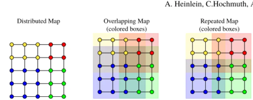
Distributed Map Overlapping Map Repeated Map

(colored boxes) (colored boxes)

Fig. 1 Sketch of the approximation of the nonoverlapping subdomains and the interface, respectively: uniquely distributed map (left); extension of the uniquely distributed map by one layer of elements resulting in an overlapping map, where the overlap contains the interface (middle); by se- lection, using the lower subdomain ID, the a map approximating to the nonoverlapping subdomains is constructed (right). Taken from [10].

FROSch, [12, 7]. The reduction of the coarse space dimension can also be seen in Table 1. There are several variants of RGDSW coarse spaces, which differ in a scaling of the interface degrees of freedom. Here, we will only consider the most algebraic variant, which is denoted as Option 1 in [5]; cf. [7] for a detailed description of our implementation of Option 1 of the RGDSW coarse space.

In our numerical simulations, we will also employ the recycling strategies pre- sented in [7]. We always reuse the symbolic factorizations from previous time or Newton iterations. Moreover, we reuse the coarse space from previous iterations and, for the dynamic problem, additionally the coarse matrix. Furthermore, as in [7], we always use a scaled first level operator with overlap

δ=

1h.

3 Fully Algebraic Construction of GDSW and RGDSW Coarse Spaces

As previously described, the construction of GDSW and RGDSW coarse spaces for elasticity problems requires both the domain decomposition interface and the null space of the operator, i.e., the rigid body motions. Here, we describe how we construct the coarse space if this information is not available.

Algebraic approximation of the interface If the distribution of the system ma-

trix is unique, the interface cannot be recovered. Therefore, we will carry out the

following process to approximate the nonoverlapping subdomains and hence the

interface. Starting from the unique distribution, we first add one layer of elements to

each subdomain. The overlap of the resulting domain decomposition now contains

the interface but also other finite element nodes. In order to reduce the number of

unnecessary nodes, we compare the subdomain ID of the original unique decom-

position and the decomposition with one layer of overlap and remove nodes from

the overlapping subdomains if the subdomain ID is lower compared to the original

decomposition; this process is sketched in [10] and Figure 1.

(6)

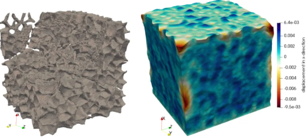
Fig. 2 Left: Slice through elements with high coefficient (µhigh =10³) displayed as a wireframe.

Low coefficient isµlow= 1; cf. [8], for a detailed discussion of the foam geometry used for an heterogeneous Poisson problem. Right: Solution of dynamic problem atT =10⁻²for∆t=10⁻³ with a warp filter and a 5 times scaling factor.

Incomplete null space The rigid body modes are the translations and rotations of the elastic body. The translations are constant functions which can be constructed without any geometric information. Since we are not able to compute the rotations from the fully assembled matrix and without coordinates of the finite element nodes, we just omit them in the fully algebraic coarse space; see also [11]. For the results in section 4, only the number of iterations is negatively effected by omitting rotations from the coarse space but the time to solution actually benefits from the smaller coarse space. Note that, from theory, the rotational basis functions are necessary for numerical scalability. Therefore, we expect that there are problems for which the full coarse space performs better.

4 Numerical Results

In this section, we compare the GDSW and RDSW preconditioners with exact

interface maps and full coarse space, GDSW and RGDSW preconditioners with exact

interface map but without rotational basis functions, and the fully algebraic variant

with approximated interface and without rotational basis functions; for the sake of

brevity, we denote the three variants as “rotations”, “no rotations”, and “algebraic”,

respectively. As discussed in section 2, we consider a stationary elasticity problem

with homogeneous shear modulus of

µ=

5

·

10

³

and a dynamic elasticity problem

with two material phases; cf. Figure 2 (left) for a graphical representation of the

coefficient distribution of the shear modulus. For both cases, we choose

ν=

0.4. For

the stationary homogeneous model problem, we use structured grids and structured

decompositions into square subdomains, whereas for the dynamic problem, we use

(7)

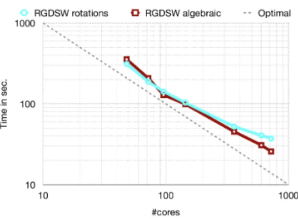
Fig. 3 Strong scaling for dynamic problem up to timeT=2·10⁻²for the foam geometry.

#cores 64 512 4 096

GDSW

rotations 1 593 16 149 144 045 no rotations 837 8 589 77 085 algebraic P1 disc. 1 395 11 355 84 762 algebraic P2 disc. 1 554 11 466 84 708 RGDSW

rotations 162 2 058 20 250 no rotations 81 1 029 10 125 algebraic P1 disc. 93 1 065 10 218 algebraic P2 disc. 93 1 038 10 134

Table 1 Comparison of coarse matrix sizes for a structured domain decomposition and the approximated subdomain maps for a P1 (H/h=21) and P2 (H/h=9) discretizaion.

a fixed unstructured tetrahedral mesh with roughly 3.3 million elements and 588 k nodes. We use the inexact Newton method of Eisenstat and Walker [6] with a type 2 forcing term until a relative residual of

_nl=

10

⁻⁸

is achieved. The initial forcing term is

η_init=

10

⁻³

and the maximum and minimum forcing terms are

η_max=

10

⁻²

and

η_min=

10

⁻⁸

, respectively. Therefore, we use a combination of the Trilinos packages

Thyra

and

NOX. Furthermore,NOX

is used for a backtracking globalization strategy. In particular, the step length is chosen as 0.5

^l

with

l =

0, 1, ... until the Armijo condition is satisfied. All linearized problems are solved with right-preconditioned GMRES with the corresponding GDSW and RGDSW preconditioners and the tolerance for the relative residual error is the forcing term

η. All computations were carried out

on the supercomputer magnitUDE of the University Duisburg-Essen, Germany.

In Tables 2 and 3, weak scaling results for the stationary model problem with

piecewise linear and piecewise quadratic elements are depicted. Although, iteration

counts are slightly higher for the RGDSW coarse spaces compared to the respective

GDSW coarse spaces, the total computation time is much smaller for RGDSW due

to the lower dimension of the coarse problem. This effect is even stronger for larger

numbers of subdomains and cores; cf. Table 1. Furthermore, we observe competitive

(8)

Prec. Type #cores 64 512 4 096

GDSW

rot. #its. 17.8 19.0 19.0

time 35.1 / 7.4 / 42.5 45.3 / 9.7 / 55.0 167.1 / 26.1 / 183.2

no rot. #its. 27.3 32.0 35.5

time 29.3 / 10.6 / 39.9 32.9 / 13.8 / 46.7 70.8 / 23.3 / 94.1

algebraic #its. 32.8 38.5 39.0

time 39.5 / 13.4 / 52.9 41.6 / 17.2 / 58.8 84.3 / 27.3 / 111.6

RGDSW

rot. #its. 20.5 22.5 22.5

time 28.8 / 8.2 / 37.0 30.9 / 9.5 / 40.4 42.0 / 11.7 / 53.7

no rot. #its. 33.0 37.3 39.5

time 25.2 / 12.4 / 37.6 26.5 / 14.7 / 41.2 30.1 / 18.0 / 48.1

algebraic #its. 40.0 42.0 43.0

time 27.2 / 15.5 / 42.7 28.7 / 16.8 / 45.5 32.9 / 19.6 / 52.5

Table 2 Stationary problem, discretization P1 (H/h=21), iteration counts are averages over all Newton iterations. All problems were solved in 4 Newton iterations. The three timings are for the setup / solve / total time and are in seconds. All total times are highlighted.

Prec. Type #cores 64 512 4 096

GDSW

rot. #its. 16.3 17.3 19.3

time 40.1 / 5.9 / 46.0 55.0 / 8.5 / 63.5 223.3 / 24.4 / 247.7

no rot. #its. 24.5 29.3 32.3

time 32.5 / 8.4 / 40.9 38.4 / 11.8 / 46.7 102.2 / 20.0 / 122.2

algebraic #its. 57.5 74.8 78.0

time 42.0 / 20.5 / 62.5 46.0 / 29.9 / 75.9 124.8 / 50.5 / 175.3

RGDSW

rot. #its. 18.8 21.3 19.8

time 27.8 / 6.4 / 34.2 31.1 / 8.0 / 39.1 41.3 / 8.9 / 50.2

no rot. #its. 29.0 32.8 35.5

time 26.2 / 9.4 / 35.6 27.3 / 11.8 / 39.1 31.1 / 14.3 / 45.4

algebraic #its. 60.7 78.5 83.0

time 27.9 / 19.9 / 47.8 28.7 / 27.9 / 56.6 34.1 / 33.1 / 67.2

Table 3 Stationary problem, discretization P2 (H/h =9), iteration counts are averages over all Newton iterations. All problems were solved in 4 Newton iterations. The three timings are for the setup / solve / total time and are in seconds. All total times are highlighted.

iteration counts and computing times when using the fully algebraic coarse spaces.

In addition to that, the approximation strategy for the interface seems to perform better for piecewise linear than for piecewise quadratic elements.

In Figure 3, we present strong scaling results from 48 to 720 cores for the dynamic model problem. The reported times are the total times for our preconditioners, i.e., the sum of the times needed for their construction and their applications in GMRES.

We solve the problem with

∆t =

10

⁻³

up to a final time

T =

2

·

10

⁻²

using the

RGDSW rotations coarse space and using the RGDSW algebraic coarse space both

with matrix recycling; cf. [7]. Here, we observe very good strong scalability results

(9)

for both variants even though the model problem has coefficient jumps. Again, the fully algebraic variant is competitive.

AcknowledgementsThe authors gratefully acknowledge financial support by the German Science Foundation (DFG), project no. 214421492 and the computing time granted by the Center for Computational Sciences and Simulation (CCSS) of the University of Duisburg-Essen and provided on the supercomputer magnitUDE (DFG grants INST 20876/209-1 FUGG, INST 20876/243-1 FUGG) at the Zentrum für Informations- und Mediendienste (ZIM). We further thank Jascha Knepper for providing the foam geometry.

References

1. X.-C. Cai and M. Sarkis. A restricted additive Schwarz preconditioner for general sparse linear systems.SIAM Journal on Scientific Computing, 21:239–247, 1999.

2. C. R. Dohrmann, A. Klawonn, and O. B. Widlund. Domain decomposition for less regular subdomains: overlapping Schwarz in two dimensions.SIAM J. Numer. Anal., 46(4):2153–2168, 2008.

3. C. R. Dohrmann, A. Klawonn, and O. B. Widlund. A family of energy minimizing coarse spaces for overlapping Schwarz preconditioners. InDomain decomposition methods in science and engineering XVII, volume 60 ofLect. Notes Comput. Sci. Eng., pages 247–254. Springer, Berlin, 2008.

4. C. R. Dohrmann and O. B. Widlund. Hybrid domain decomposition algorithms for compress- ible and almost incompressible elasticity. Internat. J. Numer. Meth. Engng, 82(2):157–183, 2010.

5. C. R. Dohrmann and O. B. Widlund. On the design of small coarse spaces for domain decomposition algorithms.SIAM J. Sci. Comput., 39(4):A1466–A1488, 2017.

6. S. C. Eisenstat and H. F. Walker. Choosing the forcing terms in an inexact Newton method.

volume 17, pages 16–32. 1996. Special issue on iterative methods in numerical linear algebra (Breckenridge, CO, 1994).

7. A. Heinlein, C. Hochmuth, and A. Klawonn. Reduced dimension GDSW coarse spaces for monolithic Schwarz domain decomposition methods for incompressible fluid flow problems.

International Journal for Numerical Methods in Engineering, n/a(n/a).

8. A. Heinlein, A. Klawonn, J. Knepper, and O. Rheinbach. Adaptive GDSW coarse spaces for overlapping Schwarz methods in three dimensions. SIAM Journal on Scientific Computing, 41(5):A3045–A3072, 2019.

9. A. Heinlein, A. Klawonn, S. Rajamanickam, and O. Rheinbach. FROSch – a parallel implementation of the GDSW domain decomposition preconditioner in Trilinos. In preparation.

10. A. Heinlein, A. Klawonn, S. Rajamanickam, and O. Rheinbach. FROSch: A Fast and Robust Overlapping Schwarz Domain Decomposition Preconditioner Based on Xpetra in Trilinos.

Technical report, Universität zu Köln, November 2018.

11. A. Heinlein, A. Klawonn, and O. Rheinbach. A parallel implementation of a two-level overlapping Schwarz method with energy-minimizing coarse space based on Trilinos.SIAM J. Sci.

Comput., 38(6):C713–C747, 2016.

12. A. Heinlein, A. Klawonn, O. Rheinbach, and O. B. Widlund. Improving the parallel performance of overlapping Schwarz methods by using a smaller energy minimizing coarse space.

International Conference on Domain Decomposition Methods, pages 383–392. Springer, 2017.

13. M. A. Heroux, R. A. Bartlett, V. E. Howle, R. J. Hoekstra, J. J. Hu, T. G. Kolda, R. B. Lehoucq, K. R. Long, R. P. Pawlowski, E. T. Phipps, A. G. Salinger, H. K. Thornquist, R. S. Tuminaro, J. M. Willenbring, A. Williams, and K. S. Stanley. An overview of the Trilinos project.ACM Trans. Math. Softw., 31(3):397–423, 2005.