Technical Report Series Center for Data and Simulation Science

Technical Report Series

Center for Data and Simulation Science

Alexander Heinlein, Axel Klawonn, Martin Lanser, Janine Weber

Predicting the geometric location of critical edges in adaptive GDSW overlapping domain decomposition methods using deep learning

Technical Report ID: CDS-2021-02

Available at https://kups.ub.uni-koeln.de/id/eprint/36257

Submitted on March 12, 2021

Predicting the geometric location of critical edges in adaptive GDSW overlapping domain decomposition methods using deep learning

Alexander Heinlein, Axel Klawonn, Martin Lanser, and Janine Weber

1 Introduction

For complex model problems with coefficient or material distributions with large jumps along or across the domain decomposition interface, the convergence rate of classic domain decomposition methods for scalar elliptic problems usually deterio- rates. In particular, the classic condition number bounds [1, 2, 13, 14] will depend on the contrast of the coefficient function. As a remedy, different adaptive coarse spaces, e.g, [15, 5], have been developed which are obtained by solving certain gen- eralized eigenvalue problems on local parts of the interface, i.e., edges and/or faces.

A selection of the resulting eigenmodes, based on a user-defined tolerance, is then used to enrich the coarse space and retain a robust convergence behavior. However, the setup and the solution of the eigenvalue problems usually take up a significant amount of time in a parallel computation, and for many realistic coefficient distribu- tions, a relatively high number of the eigenvalue problems is unnecessary since they do not result in any additional coarse basis functions. Unfortunately, it is not known a priori, which eigenvalue problems are unnecessary and thus can be omitted.

In order to reduce the number of eigenvalue problems, we have proposed to train a neural network to make an automatic decision which of the eigenvalue problems can be omitted in a preprocessing step. In [7, 10, 8], we have applied this Alexander Heinlein

Institute of Applied Analysis and Numerical Simulation, Universität Stuttgart,

Pfaffenwaldring 57, 70569 Stuttgart, Germany, e-mail: Alexander.Heinlein@ians.uni-stuttgart.de Axel Klawonn, Martin Lanser

Department of Mathematics and Computer Science, University of Cologne, Weyertal 86-90, 50931 Köln, Germany, e-mail: axel.klawonn@uni-koeln.de, martin.lanser@uni-koeln.de, url:

http://www.numerik.uni-koeln.de

Center for Data and Simulation Science, University of Cologne, url: http://www.cds.uni-koeln.de Janine Weber

Department of Mathematics and Computer Science, University of Cologne, Weyertal 86-90, 50931 Köln, Germany, e-mail: janine.weber@uni-koeln.de, url: http://www.numerik.uni-koeln.de

1

2 Alexander Heinlein, Axel Klawonn, Martin Lanser, and Janine Weber approach to a certain adaptive FETI-DP (Finite Element Tearing and Interconnecting - Dual Primal) method [15] for elliptic model problems in two dimensions and investigated the effect of different training data sets and different sizes of input data for the neural network. In [6], we have additionally extended our approach to three-dimensional model problems for the corresponding adaptive FETI-DP method in three dimensions [12]. In [11], for the first time, we additionally applied our proposed machine learning framework to an overlapping domain decomposition method, i.e., the adaptive GDSW (Generalized Dryja-Smith-Widlund) method [4].

The purpose of [11] was to provide a general overview of methods combining machine learning with domain decomposition methods, and thus, we have solely presented some preliminary results for adaptive GDSW. Here, we extend the results shown in [11] by providing numerical experiments for additional test problems.

Furthermore, we take a closer look at the choice of the ML threshold which is used for the classification between critical edges, for which the eigenvalue problem is necessary, and edges where the eigenvalue problem can be omitted. The specific choice of the threshold is now, for the first time, motivated by the corresponding receiver operating characteristic (ROC) curve and the precision-recall graph.

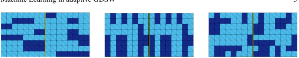
We focus on a stationary diffusion problem in two dimensions and the adaptive GDSW method [4]. The diffusion coefficient function is defined on the basis of different subsections of a microsection of a dual-phase steel material.

2 Model Problem and Adaptive GDSW

As a model problem, we consider a stationary diffusion problem in two dimensions with various heterogeneous coefficient functions d : ⌦ := [ 0, 1 ] ⇥ [ 0, 1 ] ! R, i.e., the weak formulation of

div ( d r D ) = 1 in ⌦

D = 0 on m⌦. (1)

In this paper, we apply the proposed machine learning-based strategy to an adaptive GDSW method. We decompose the domain ⌦ into # 2 N nonoverlapping subdo- mains ⌦

, 8 = 1, . . . , #, such that ⌦ = –

8=1

⌦

. Next, we introduce overlapping subdomains ⌦

, 8 = 1, ..., #, which can be obtained from ⌦

, 8 = 1, ..., # by re- cursively adding : layers of finite elements. In the numerical experiments presented in this paper, we always choose an overlap of width X = ⌘; this corresponds to choosing : = 1. Due to space limitations, we do not describe the standard GDSW preconditioner in detail; see, e.g., [1, 2] for a detailed description.

As discussed in [5], the condition number bound for the standard GDSW precon-

ditioner generally depends on the contrast of the coefficient function for completely

arbitrary coefficient distributions. As a remedy, additional coarse basis functions re-

sulting from the eigenmodes of local generalized eigenvalue problems are employed

to compute an adaptive coarse space which is robust and yields a coefficient contrast-

independent condition number bound. In two dimensions, each of these eigenvalue

problems is associated with a single edge and its two neighboring subdomains. Thus, the main idea for the adaptive GDSW (AGDSW) coarse space [4] is to build edge basis functions based on local generalized eigenvalue problems. In particular, the coarse basis functions are defined as discrete harmonic extensions of certain corre- sponding edge eigenmodes. The specific eigenmodes which are necessary to retain a robust convergence behavior are chosen depending on a user-defined tolerance C>;

0, which has to be chosen in relation to the spectrum of the preconditioned system. For a detailed description of the specific local edge eigenvalue problems and the computation of the discrete harmonic extensions, we refer to [4]. In particular, in the AGDSW approach, all eigenmodes with eigenvalues lower or equal to C>;

are chosen to build the adaptive coarse space. Since the left-hand side of the edge eigenvalue problem is singular (cf. [4, Sec. 5]), for each edge, we always obtain one eigenvalue equal to zero. It corresponds to the null space of the Neumann matrix of (1), which consists of the constant functions. The corresponding coarse basis function is also part of the standard GDSW coarse space, and we denote it as the first coarse basis function in this paper. Let us note that the first coarse basis func- tion is always necessary for the scalability of the approach, even for the case of a constant coefficient function. However, since it corresponds to the constant function on the edge, it is known a priori and can be computed without actually solving the eigenvalue problem.

As for most adaptive domain decomposition methods, for AGDSW, it is generally not known a priori on which edges additional coarse basis functions are necessary in order to obtain robustness. In general, building the adaptive coarse space, i.e, the setup and the solution of the eigenvalue problems as well as the computation of the discrete harmonic extensions, can make up the larger part of the time to solution in a parallel implementation. Since the computation of the adaptive GDSW coarse space is - similarly to the adaptive FETI-DP methods - based on local eigenvalue problems associated with edges, we can apply the same machine learning strategy introduced in [7, 10] to predict the location of necessary eigenvalue problems.

3 Machine Learning for Adaptive GDSW

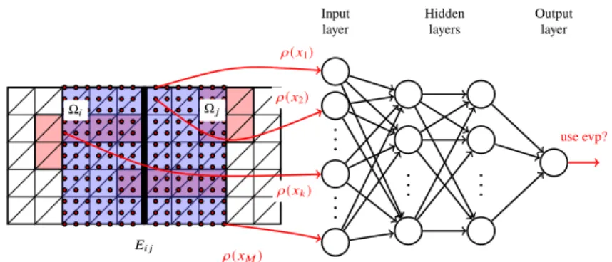
Our approach is to train a neural network to make an automatic decision whether it is necessary to solve a local eigenvalue problem for a specific edge to retain a robust AGDSW algorithm. We denote this approach, which is inspired by the ML-FETI- DP approach introduced in [7, 10], as ML-AGDSW. In particular, we use a dense feedforward neural network, or more precisely, a multilayer perceptron [16, 3] to make this decision. Since each eigenvalue problem for AGDSW is associated with a single edge and both neighboring subdomains, we use samples of the coefficient function within the two adjacent subdomains as input data for the neural network;

cf. fig. 1. In particular, we apply a sampling approach which is independent of

the finite element mesh, using a fixed number of sampling points for all mesh

resolutions; this is reasonable as long as we can resolve all geometric features of the

4 Alexander Heinlein, Axel Klawonn, Martin Lanser, and Janine Weber

⌦8 ⌦9

⇢8 9

.. . .. .

.. . .. .

Input

layer Hidden

layers Output

layer d(G1)

d(G2)

d(G:)

d(G")

use evp?

Fig. 1 Sampling of the coefficient function; white color corresponds to a low coefficient and red color to a high coefficient. In this representation, the samples are used as input data for a neural network with two hidden layers. Only sampling points from slabs around the edge are chosen. Taken from [8, Fig. 1].

coefficient function. For more details on the computation of the sampling grid and its generalization to more general subdomain geometries than square subdomains, see [7].

As output for the neural network, we save the classification whether an adaptive basis function has to be computed for the specific edge or not. As already mentioned, in AGDSW, the first coarse basis function is always necessary but can be computed without actually solving the eigenvalue problem. Hence, an eigenvalue problem will only be marked as necessary in our approach if more than one coarse basis function corresponds to an eigenvalue lower than the chosen tolerance C>;

. Therefore, for ML-AGDSW, all critical edges, where more than the single constant constraint is necessary, are classified as class 1. All other edges are classified as class 0. Let us note that this is different to the definition of class 1 for ML-FETI-DP introduced in [7, 10], where the eigenvalue 0 corresponding to the constant functions does not occur in the eigenvalue problem.

For the numerical results presented in this paper, we train the neural network on two regular subdomains sharing a straight edge and different types of coefficient functions. Using the same techniques as in [10, 11], we have generated a training and validation data set of 4 500 randomized coefficient distributions. In particular, the coefficient distributions are not completely random but we impose some sort of structure on the coefficients; see also [10] for a detailed discussion. For the first part of this training set, we randomly generate the coefficient for each pixel, consisting of two triangular finite elements, independently and only control the ratio of high and low coefficient values. Here, we use 30%, 20%, 10%, and 5% of high coefficient values.

For the second part, we also control the distribution of the coefficients to a certain

degree by randomly generating either horizontal or vertical stripes of a maximum

length of four or eight pixels, respectively; see Figure fig. 2. Additionally, we generate

new coefficient distributions by superimposing pairs of coefficient distributions with

horizontal and vertical stripes. We denote the resulting training data set by R1’. Let

us note that the generation of the randomized coefficient distributions as training

Fig. 2 Examples of three different randomly distributed coefficient functions obtained by using the same randomly generated coefficient for a horizontal (left) or vertical (middle) stripe of a maximum length of four finite element pixels, as well as by pairwise superimposing (right).

data for AGDSW is in complete analogy to our randomized training data for the ML-FETI-DP approach in [10]. However, we explicitly built a separate set of labels for the training and validation data for AGDSW since the classification of critical edges can be different for adaptive GDSW and adaptive FETI-DP.

To generate the output data for the neural network, we solve the eigenvalue prob- lem as described in [5] for each edge in the aforementioned training and validation data. For all our training and validation data, we use a tolerance of C>;

= 0.01 to generate the output for each edge.

Note that, for ML-FETI-DP, we additionally considered the extension to three classes, where we distinguished between zero, one, or more than one constraints.

For the edges which require only one constraint, we used frugal constraints [9]

instead of solving the eigenvalue problem; see [7] for more details. Consequently, the eigenvalue problem only had to be solved for edges with more than one constraint.

However, this approach does not easily extend to AGDSW since we always obtain at least one a priori known coarse basis function on each edge; as mentioned earlier, we always obtain a constant eigenfunction corresponding to eigenvalue 0.

4 Numerical Results

In this section, we apply our machine learning approach to AGDSW. We will present numerical results both for the training and validation data as well as for a specific test problem and compare the resulting condition number estimates and iteration counts with those obtained using both standard and adaptive GDSW; we use pcg with a relative residual reduction of 14 8. For the numerical experiments, we consider a discretization of the model problem eq. (1) by piecewise linear finite elements.

First, we present results for the complete set of training data R1’ using cross-

validation and a fixed ratio of 20% validation data in table 1. We observe that

choosing the ML threshold as g = 0.5 to distinguish between class 0 and 1, i.e.,

assuming an equal distribution among the two classes, results in an accuracy which

is comparable to the corresponding ML-FETI-DP approach; see [10, 11]. Besides

the accuracy values for the training data in table 1, we also provide the ROC curve

and a precision-recall plot in fig. 3. Both curves provide an evidence whether we

obtain a reliable machine learning model [16, Sec. 5]. As mentioned in section 3,

our aim is to identify all critical edges where an adaptive coarse basis function is

6 Alexander Heinlein, Axel Klawonn, Martin Lanser, and Janine Weber training configuration threshold fp fn acc

R1’, full sampling 0.4 11.5% 2.7% 85.8%

0.5 6.7% 7.1% 86.2%

Table 1 Results on the complete training data set for the GDSW method and stationary diffusion;

the numbers are averages over all training configurations. See table 2 for the column labeling.

necessary for robustness. For the remainder of this paper, we will refer to these critical edges as ’positive’ or ’positive edges’ and to edges where the eigenvalue problem is unnecessary as ’negative’ or ’negative edges’.Thus, only false negative edges are critical for the convergence of ML-AGDSW, whereas false positive edges correspond to some unnecessary eigenvalue problems. increases the computational effort of our algorithm but does not negatively affect its convergence behavior; note that the additionally computed eigenfunctions will not enter the coarse space since the tolerance criterion will not be satisfied. When considering the precision-recall plot in fig. 3 (right) we observe that using the ML threshold g = 0.4 compared to g = 0.45 results in a higher recall for the validation data while preserving nearly the same precision value. This is caused by a decrease in the number of false negative edges compared to g = 0.45. Moreover, the precision for both training and validation data strongly decreases when using ML thresholds smaller than 0.4. Since our predominant aim is to avoid false negative edges while still preserving a sufficient accuracy of the classification, using the ML threshold g = 0.4 seems to work best for our purpose. Besides, for g = 0.4 the ROC curve for the validation data in fig. 3 (left) is close to the respective curve for the training data which suggests that we obtain a model with good generalization properties. We will thus use g = 0.4 for the classification of our test problems and also provide comparative results for g = 0.5.

As a test problem for our trained neural network, we use 10 different randomly chosen subsections of a microsection of a dual-phase steel as shown in fig. 4 (right). In all presented computations, we consider d = 146 in the black part of the microsection and d = 1 elsewhere. We use a regular decomposition of the domain ⌦ := [ 0, 1 ] ⇥ [ 0, 1 ] into 8 ⇥ 8 square subdomains with an overlap of X = ⌘, a subdomain size of / ⌘ = 56, and a tolerance of C>;

= 0 . 01. For the test data, we only solve the local eigenvalue problem on edges which are classified as class 1 by the neural network. For all edges classified as class 0, we do not solve the eigenvalue problem and only enforce the constant constraint on the respective edge. When considering the results for one specific mircosection in table 2 as well as the average values for all 10 different subsections in table 3, we observe that, in both cases, we are able to obtain no false negative edges for the classification using the ML threshold g = 0.4.

Analogously to the training and validation data in table 1, using the lower threshold

g = 0.4 compared to g = 0.5 decreases the false negative rate of the predictions and

thus increases the robustness of our algorithm. In particular, in table 3, we obtain

zero false negative edges for all 10 different microsection subsections when using

g = 0.4. On the other hand, on average, we only solve 5.2 unnecessary eigenvalue

problems. This implies that our framework is robust for different heterogeneous

coefficient distributions and can successfully be applied to AGDSW.

Fig. 3 ROC curve (left) and precision-recall plot (right) for the ML-AGDSW method. We define precision as true positives divided by (true positives+false positives), and recall as true positives divided by (true positives+false negatives). The thresholds used in section 4 are indicated as circles.

Model Problem Algorithm

cond it evp fp fn acc standard GDSW - 3.66e06 500 0 - - - Microsection adaptive GDSW - 162.60 95 112 - - - Problem ML-AGDSW 0.5 9.64e4 98 25 2 2 0.95 ML-AGDSW 0.4 163.21 95 29 6 0 0.95

Table 2 Comparison of standard GDSW, adaptive GDSW, and ML-AGDSW for a regular domain decomposition with

subdomains and

for the two-class model, with

We show the ML threshold (g), the condition number (cond), the number of CG iterations (it), the number of solved eigenvalue problems (evp), the number of false positives (fp), the number of false negatives (fn), and the accuracy in the classification (acc). We define the accuracy (acc) as the number of true positives and true negatives divided by the total number of edges.

Alg.

cond it evp fp fn acc

standard - 4.7e06 (5.11e06) 511.2 (518) 0 - - -

adaptive - 178.6 ( 181.4) 87.2 ( 98) 112.0 (112) - - - ML-AGDSW 0.5 7.8e04 (9.2e04) 92.2 (102) 26.4 ( 29) 1.6 (2) 1.8 (3) 0.96 (0.95) 0.4 178.7 ( 181.4) 87.3 ( 98) 33.4 ( 36) 5.2 (8) 0 (0) 0.95 (0.94) Table 3 Comparison of standard GDSW, adaptive GDSW, and ML-AGDSW for a regular domain decomposition with

subdomains and

for the two-class model, with

for 10 different subsections of the microsection in fig. 4 (right) for a stationary diffusion problem.

See table 2 for the column labeling.

References

1. C. R. Dohrmann, A. Klawonn, and O. B. Widlund. Domain decomposition for less regular subdomains: overlapping Schwarz in two dimensions. SIAM J. Numer. Anal., 46(4):2153–2168, 2008.

2. C. R. Dohrmann, A. Klawonn, and O. B. Widlund. A family of energy minimizing coarse

spaces for overlapping Schwarz preconditioners. In Domain decomposition methods in science

and engineering XVII, volume 60 of LNSCE, pages 247–254. Springer, Berlin, 2008.

8 Alexander Heinlein, Axel Klawonn, Martin Lanser, and Janine Weber

Fig. 4 Left: Subsection of a microsection of a dual-phase steel obtained from the image on the right.

We consider

in the black part and

elsewhere. Right: Complete microsection of a dual-phase steel. Right image: Courtesy of Jörg Schröder, University of Duisburg-Essen, Germany, orginating from a cooperation with ThyssenKruppSteel.

3. I. Goodfellow, Y. Bengio, A. Courville, and Y. Bengio. Deep learning, volume 1. MIT press Cambridge, 2016.

4. A. Heinlein, A. Klawonn, J. Knepper, and O. Rheinbach. An adaptive GDSW coarse space for two-level overlapping Schwarz methods in two dimensions. In Domain Decomp. Meth. Sci.

Eng. XXIV, volume 125 of LNCSE, pages 373–382. Springer, Cham, 2018.

5. A. Heinlein, A. Klawonn, J. Knepper, and O. Rheinbach. Adaptive GDSW Coarse Spaces for Overlapping Schwarz Methods in Three Dimensions. SIAM J. Sci. Comput., 41(5):A3045–

A3072, 2019.

6. A. Heinlein, A. Klawonn, M. Lanser, and J. Weber. Combining Machine Learning and Adaptive Coarse Spaces - A Hybrid Approach for Robust FETI-DP Methods in Three Dimensions.

2019. TR series, Center for Data and Simulation Science, University of Cologne, Germany, Vol. 2020-1. https://kups.ub.uni-koeln.de/id/eprint/11285. Submitted June 2020.

7. A. Heinlein, A. Klawonn, M. Lanser, and J. Weber. Machine Learning in Adaptive Domain Decomposition Methods - Predicting the Geometric Location of Constraints. SIAM J. Sci.

Comput., 41(6):A3887–A3912, 2019.

8. A. Heinlein, A. Klawonn, M. Lanser, and J. Weber. Machine Learning in Adaptive FETI-DP - Reducing the Effort in Sampling. 2019. TR series, Center for Data and Simulation Science, University of Cologne, Germany, Vol. 2019-19. http://kups.ub.uni-koeln.de/id/eprint/10439.

Proceedings of the ENUMATH 2019 conference, Springer LNCSE. Accepted May 2020.

9. A. Heinlein, A. Klawonn, M. Lanser, and J. Weber. A Frugal FETI-DP and BDDC Coarse Space for Heterogeneous Problems. Electr. Trans. Numer. Anal., 53:562–591, 2020.

10. A. Heinlein, A. Klawonn, M. Lanser, and J. Weber. Machine Learning in Adaptive FETI-DP - A Comparison of Smart and Random Training Data. In Domain Decomposition Methods in Science and Engineering XXV, volume 138 of LNCSE, pages 218–226. Springer, Cham, 2020.

11. A. Heinlein, A. Klawonn, M. Lanser, and J. Weber. Combining Machine Learning and Domain Decomposition Methods - A Review. GAMM Mitteilungen (accepted for publication), 2021.

TR series, Center for Data and Simulation Science, University of Cologne, Germany, Vol.

2020-9. https://kups.ub.uni-koeln.de/id/eprint/20708. Submitted October 2020.

12. A. Klawonn, M. Kühn, and O. Rheinbach. Adaptive coarse spaces for FETI-DP in three dimensions. SIAM J. Sci. Comput., 38(5):A2880–A2911, 2016.

13. A. Klawonn, O. Rheinbach, and O. B. Widlund. An analysis of a FETI-DP algorithm on irregular subdomains in the plane. SIAM J. Numer. Anal., 46(5):2484–2504, 2008.

14. A. Klawonn and O. B. Widlund. Dual-primal FETI methods for linear elasticity. Comm. Pure Appl. Math., 59(11):1523–1572, 2006.

15. J. Mandel and B. Sousedík. Adaptive selection of face coarse degrees of freedom in the BDDC and the FETI-DP iterative substructuring methods. Comput. Methods Appl. Mech. Engrg., 196(8):1389–1399, 2007.

16. A. Müller and S. Guido. Introduction to Machine Learning with Python: A Guide for Data

Scientists. O’Reilly Media, 2016.