Technical Report Series
Center for Data and Simulation Science
Alexander Heinlein, Axel Klawonn, Martin Lanser, Janine Weber
Combining Machine Learning and Adaptive Coarse Spaces - A Hy- brid Approach for Robust FETI-DP Methods in Three Dimensions
Technical Report ID: CDS-2020-1
Available at https://kups.ub.uni-koeln.de/id/eprint/11285
Submitted on June 16, 2020
SPACES – A HYBRID APPROACH FOR ROBUST FETI-DP
2
METHODS IN THREE DIMENSIONS
3
ALEXANDER HEINLEIN∗†, AXEL KLAWONN∗†, MARTIN LANSER∗†, AND JANINE 4
WEBER∗ 5
June 16, 2020
6
Abstract. The hybrid ML-FETI-DP algorithm combines the advantages of adaptive coarse 7
spaces in domain decomposition methods and certain supervised machine learning techniques. Adap- 8
tive coarse spaces ensure robustness of highly scalable domain decomposition solvers, even for highly 9
heterogeneous coefficient distributions with arbitrary coefficient jumps. However, their construction 10
requires the setup and solution of local generalized eigenvalue problems, which is typically compu- 11
tationally expensive. The idea of ML-FETI-DP is to interpret the coefficient distribution as image 12
data and predict whether an eigenvalue problem has to be solved or can be neglected while still 13
maintaining robustness of the adaptive FETI-DP method. For this purpose, neural networks are 14
used as image classifiers. In the present work, the ML-FETI-DP algorithm is extended to three di- 15
mensions, which requires both a complex data preprocessing procedure to construct consistent input 16
data for the neural network as well as a representative training and validation data set to ensure 17
generalization properties of the machine learning model. Numerical experiments for stationary dif- 18
fusion and linear elasticity problems with realistic coefficient distributions show that a large number 19
of eigenvalue problems can be saved; in the best case of the numerical results presented here, 97 % 20
of the eigenvalue problems can be avoided to be set up and solved.
21
Key words. ML-FETI-DP, FETI-DP, machine learning, domain decomposition methods, adap- 22
tive coarse spaces, finite elements 23
AMS subject classifications. 65F10, 65N30, 65N55, 68T05 24
1. Introduction. Domain decomposition methods are highly scalable, iterative
25
solvers for the solution of large systems of equations such as arriving, e.g., from the
26
discretization of partial differential equations by finite elements. Among the most
27
commonly used domain decomposition methods are the FETI-DP (Finite Element
28
Tearing and Interconnecting - Dual Primal) [12, 11, 48, 49], BDDC (Balancing Do-
29
main Decomposition by Constraints) [7, 8, 51, 53, 52] and overlapping Schwarz [61]
30
methods. All of these methods have successfully been applied to a wide range of
31
problems and have been shown to be parallel scalable up to hundred of thousands
32
of cores and beyond [26, 62, 2, 1, 39, 44, 40, 38, 37, 27]. In the present article,
33
we are mostly interested in the solution of highly heterogeneous stationary diffusion
34
or linear elasticity problems with high contrasts in the material distributions. For
35
such cases, including those with arbitrary jumps in the diffusion coefficient or the
36
Young modulus, the convergence rate of standard domain decomposition methods
37
typically deteriorates severely. In particular, the classic condition number bounds for
38
standard domain decomposition methods are only valid under relatively restrictive
39
assumptions concerning the coefficient function or the material distribution. Thus, in
40
case of highly complex coefficient functions, coarse space enhancements are necessary
41
to guarantee a robust algorithm while retaining a good condition number bound to
42
preserve numerical scalability. For FETI-DP algorithms considered in the present
43
∗Department of Mathematics and Computer Science, University of Cologne, Weyer- tal 86-90, 50931 K¨oln, Germany, alexander.heinlein@uni-koeln.de, axel.klawonn@uni-koeln.de, martin.lanser@uni-koeln.de, janine.weber@uni-koeln.de, url: http://www.numerik.uni-koeln.de
†Center for Data and Simulation Science, University of Cologne, Germany, url:http://www.cds.
uni-koeln.de
article, such a condition number bound would only depend polylogarithmically on
44
the size of the subproblems while being independent of the contrast of the values of
45
the relevant coefficient functions. To accomplish this in three dimensions for material
46
discontinuities aligned with the interface between subdomains, additional averages
47
along edges and first order moments to enhance the coarse space have been pro-
48
posed in [48, 49]. This approach has been heuristically extended in [43] for material
49
discontinuities not aligned with the interface using certain weighted averages. We
50
have further generalized this technique in [23]. Here, we have integrated general-
51
ized weighted averages along faces and/or edges into the coarse space. Using this
52
approach as a default can help to make FETI-DP and BDDC algorithms more ro-
53
bust for a number of realistic application problems. However, all aforementioned
54
approaches are generally not robust for arbitrary coefficient functions, e.g., with nu-
55
merous discontinuities along and across the interface between subdomains. Hence,
56
adaptive coarse spaces have been developed for different domain decomposition algo-
57
rithms [4,35, 34,33,58,57, 3,6,54,55,42, 41,31,13,14,10, 9,59, 60,19,18,20].
58
In adaptive coarse spaces, eigenvectors originating from the solution of certain local
59
generalized eigenvalue problems on parts of the interface, e.g., faces or edges, are used
60
to enhance the coarse space. For these techniques, condition number bounds that are
61
robust with respect to arbitrary coefficient distributions can be proven. In particular,
62
the resulting condition number bounds only depend on a user-defined tolerance, which
63
is used as a threshold for the selection of the eigenvectors based on their corresponding
64
eigenvalues, and on geometrical constants. As a drawback, in a parallel implemen-
65
tation, the setup and the solution of the eigenvalue problems take up a significant
66
amount of time; cf. [50, 36]. However, for many realistic coefficient distributions, a
67
large number of eigenvalue problems which are not necessary for a robust convergence
68
of the adaptive domain decomposition method is solved; they are not necessary in the
69
sense that no corresponding eigenvectors are being selected. In order to account for
70
this, in [24], we introduced the concept of training a neural network to make an auto-
71
matic decision whether the solution of a specific local eigenvalue problem is necessary
72
for robustness. In particular, we have focused on the two-dimensional case and the
73
adaptive coarse space introduced in [54] for the FETI-DP method, which is based
74
on local eigenvalue problems on edges between neighboring subdomains; see [42] for
75
the first theoretical proof of a robust condition number bound for this algorithm.
76
We were able to significantly reduce the number of necessary eigenvalue problems on
77
edges by using samples of the coefficient function in the adjacent subdomains as input
78
for the machine learning model; in [25], we have shown that it is actually sufficient to
79
sample in neighborhoods close to the edges. Throughout this paper, we denote the
80
algorithm combining adaptive FETI-DP and machine learning introduced in [24] by
81
ML-FETI-DP.
82
Here, we extend the two-dimensional ML-FETI-DP approach [24] to three-dimen-
83
sional problems. The main concept is very similar, however, the interface between
84
the adaptive FETI-DP algorithm and the neural network, i.e., the preprocessing of
85
the input data for the neural network, requires substantial modifications and en-
86
hancements. In particular, handling faces of three-dimensional unstructured domain
87
decompositions, e.g., obtained from METIS [30], is much more complex compared
88
to edges in two dimensions. Moreover, in the generation of training and validation
89
data, we use METIS domain decompositions and adapt the generation of coefficient
90
distributions based on randomization as described for two dimensions in [24] to three
91
dimensions. The main focus of this paper is thus on the description of the prepro-
92
cessing of the data. As a machine learning approach, we will again - as in [24] -
93
employ feedforward neural networks with Rectified Linear Unit (ReLU) activation
94
and dropout layers.
95
The remainder of this paper is organized as follows. First, we introduce our
96
model problems, namely stationary diffusion problems and linear elasticity problems.
97
Second, we briefly recapitulate the FETI-DP domain decomposition method and the
98
specific adaptive coarse space approach [33,54,55] for three dimensions. Afterwards,
99
we present our machine learning based approach ML-FETI-DP using feedforward
100
neural networks. We then describe the preprocessing of the input data and how we
101
generate appropriate training and validation data for the training process of the neural
102
network. Finally, we show numerical results for different relevant elliptic problems. At
103
first, we consider a coefficient distribution with five balls of different radii in the unit
104
cube. Second, we consider an RVE (Representative Volume Element) representing
105
the microstructure of a dual-phase steel.
106
2. Model problems and adaptive FETI-DP domain decomposition al-
107
gorithms. In this section, we give a brief introduction of our model problems and
108
shortly describe the classic FETI-DP domain decomposition method [12,11,48,49].
109
Finally, insubsection 2.3.2, we describe the employed adaptive FETI-DP coarse space
110
technique for three dimensions; see [33,54, 55].
111
2.1. Diffusion, elasticity, and finite elements. As a first model problem,
112
we consider a stationary, linear, scalar diffusion problem with a highly heterogeneous
113
coefficient functionρ: Ω→Rand homogeneous Dirichlet boundary conditions on∂Ω.
114
Thus, the model problem in its variational form can be written as: find u∈H01(Ω)
115
such that
116
(2.1)
Z
Ω
ρ∇u· ∇v dx= Z
Ω
f v dx∀v∈H01(Ω).
117
Various examples of coefficient functions are discussed insection 4.
118
As a second model problem, we consider the equations of linear elasticity. It
119
consists of finding the displacementu∈H10(Ω) := (H01(Ω))3such that
120
(2.2)
Z
Ω
G ε(u) :ε(v)dx+ Z
Ω
Gβ divudivvdx= Z
Ω
fTvdx
121
for allv∈H10(Ω), given material functions G: Ω→Randβ : Ω→R, and a volume
122
forcef ∈(L2(Ω))3.
123
By a finite element discretization of (2.1) and (2.2) on Ω, we obtain the respective
124
linear system of equations
125
(2.3) Kgug=fg.
126
We denote the finite element space by Vh and we have ug, fg ∈ Vh. Note that,
127
throughout this paper, we assume that the coefficient functions ρ, G, and β are
128
constant on each finite element but may have large jumps from element to element.
129
For simplicity, in the present article, we only consider tetrahedrons and linear finite
130
elements.
131
2.2. Standard FETI-DP. Let us briefly describe the classic FETI-DP method
132
and introduce some necessary notation.
133
2.2.1. Domain decomposition. We assume a decomposition of Ω intoN ∈N
134
nonoverlapping subdomains Ωi, i = 1, ..., N, i.e., Ω = SN
i=1Ωi. Each of the sub-
135
domains is a union of finite elements. The finite element subspaces associated with
136
Ωi, i= 1, ..., N, are denoted byWi, i= 1, ..., N. We obtain local finite element prob-
137
lemsK(i)u(i)=f(i)withK(i):Wi→Wi andf(i)∈Wi by restricting the considered
138
differential equation (2.1)or (2.2) to Ωi and discretizing its variational formulation
139
in the finite element spaceWi. Let us remark that the matricesK(i)are, in general,
140
not invertible for subdomains, which have no contact to the Dirichlet boundary.
141
We introduce the simple restriction operators Ri : Vh → Wi, i = 1, ..., N, the
142
block vectors uT := u(1)T, ..., u(N)T
and fT := f(1)T, ..., f(N)T
, and the block
143
matrices RT := RT1, ..., RTN
and K = diag K(1), ..., K(N)
. We then obtain the
144
identities
145
(2.4) Kg=RTKR and fg=RTf.
146
The application ofRT in(2.4)thus has the effect of a finite element assembly process
147
of local finite element functions on the interface Γ :=
SN i=1∂Ωi
\∂Ω.
148
The block matrixKis not invertible as soon as a single subdomain has no contact
149
to the Dirichlet boundary. Therefore, the systemKu=f has no unique solution and,
150
more precisely, an unknown vector u might be discontinuous on the interface. We
151
now proceed to describe how the solutionugis obtained using FETI-DP, i.e., how the
152
continuity ofu∈W :=W1×...×WN on the interface is enforced.
153
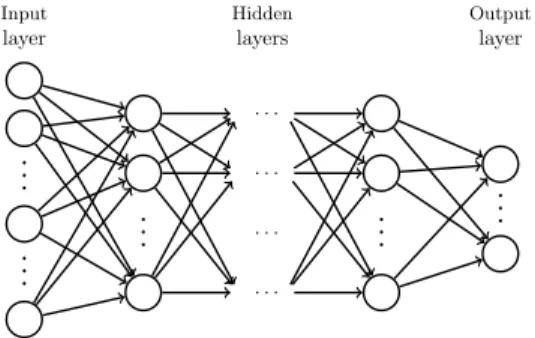
2.2.2. The FETI-DP saddle point system. Let us assume, we have sorted
154
and decomposed an unknown vectorufrom the product spaceW into interface vari-
155
ablesuΓand all remaining interior variablesuI, i.e.,uT = uTI, uTΓ
∈W. We further
156
subdivide the degrees of freedoms on the interface uΓ into primal variablesuΠ and
157
dual variables u∆. Throughout this paper, we select all subdomain vertices to be
158
primal. Continuity in the primal variables is enforced by a finite element assembly
159
process, while continuity in the dual variables is enforced iteratively by Lagrange
160
multipliers.
161
For the primal assembly process we introduce the operatorRTΠ, which is similar
162
toRT, but assembles only in primal variables. We denote the corresponding primally
163
assembled finite element space byWf. Thus, we haveRΠ:fW →W and any ˜u∈Wf
164
is of the structure ˜uT = uTI, uT∆,u˜TΠ
, where ˜uΠ is now a vector of global variables.
165
The vector ˜uΠ can also be seen as a coarse solution and the corresponding Schur
166
complement system in the primal variables constitutes the global coarse problem or
167
second level problem in FETI-DP. We define primally coupled operators by
168
(2.5) f˜=RTΠf and Ke =RΠTKRΠ.
169
Let us remark thatKe :Wf→fW will be a regular matrix if enough primal constraints
170
are chosen.
171
Enforcing continuity in the dual variables is done by the constraintBu˜= 0, using
172
a linear jump operatorB = [B(1), ..., B(N)]; see, e.g., [44] for a detailed definition of
173
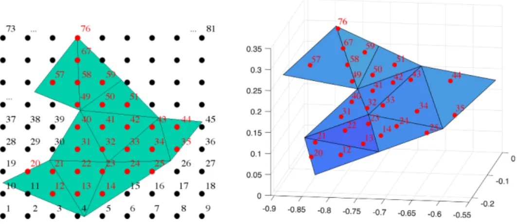
B. Each row ofBevaluates the jump between two degrees of freedom on the interface
174
belonging to the same physical node but different subdomains. Thus, each row ofB
175
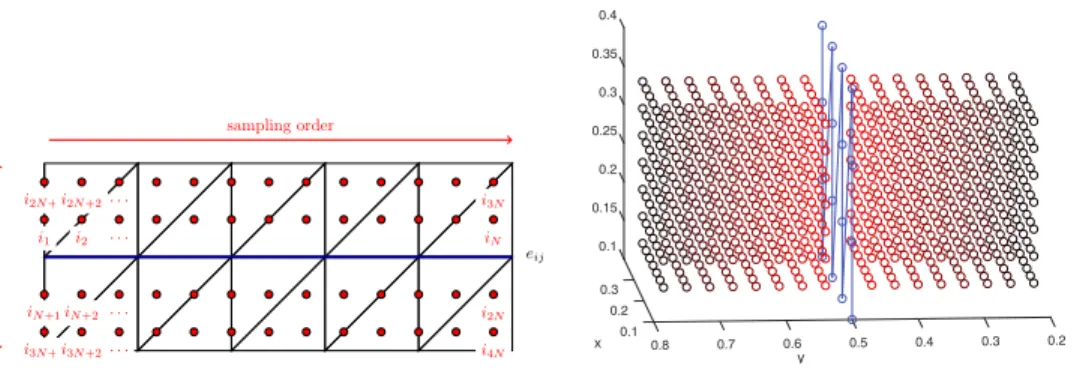
contains exactly one 1 and one−1 and the remaining entries are zero. Enforcing the
176
jump condition via Lagrange multipliers, we obtain the FETI-DP saddle point system
177
(2.6)
Ke BT
B 0
˜ u λ
= f˜
0
,
178
where λ is the vector of the Lagrange multipliers. Let us remark that, due to the
179
constraintBu˜= 0, the solution ˜u∈fW is continuous on the interface Γ.
180
2.2.3. Iterative solution of the FETI-DP system. By a block elimination
181
in(2.6)we derive the system
182
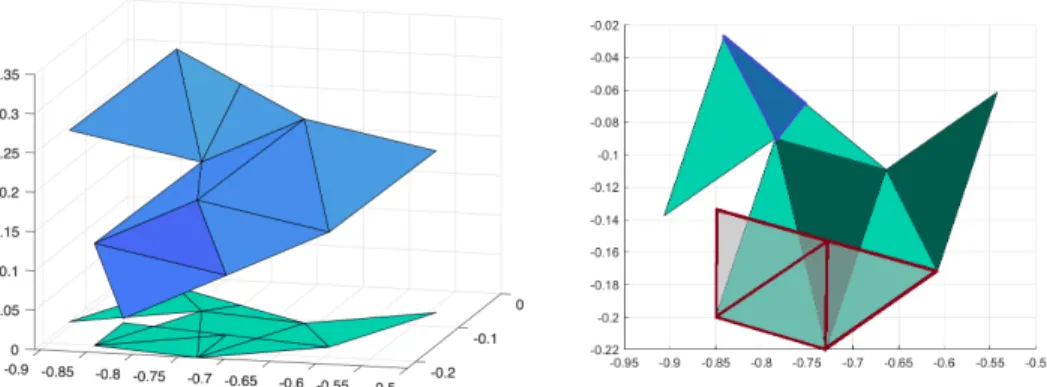
(2.7) F λ=d
183
with F = BKe−1BT and d = BKe−1f˜. Equation (2.7) is solved iteratively with a
184
preconditioned CG or GMRES approach using an additional Dirichlet preconditioner
185
MD−1; see also [61]. The preconditionerMD−1 is a weighted sum of local Schur com-
186
plements in the dual variables. Let
187
(2.8) S∆∆(i) =K∆∆(i) −K∆I(i)KII(i)−1K∆I(i)T
188
be the Schur complement ofK(i), i= 1, ..., N in the dual variables and
189
(2.9) BD=
D(1)TB(1), ..., D(N)B(N)T
190
a scaled jump matrix, where the scaling matricesD(i), i= 1, ..., Nare usually defined
191
by the PDE coefficients. We further define BD,∆, the restriction ofBD to the dual
192
variables, andS∆∆= diag(S∆∆(1), ..., S(N∆∆)). The preconditioner is then defined by
193
(2.10) MD−1=BD,∆S∆∆BD,∆T .
194
The application ofMD−1is embarrassingly parallel due to the block diagonal structure
195
ofS. The desired solution ˜uis finally obtained by solving
196
(2.11) Keu˜= ˜f −BTλ.
197
2.2.4. Condition number bound. For scalar elliptic partial differential equa-
198
tions as well as for linear elasticity problems, the classic polylogarithmic condition
199
number bound
200
(2.12) κ(MD−1F)≤C
1 + log
H h
2
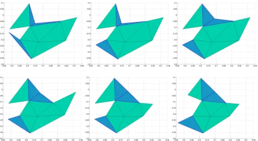
201
holds, with C independent of H and h; see, e.g., [47, 49, 48]. In (2.12) H is the
202
maximum diameter over all subdomains,hthe maximum diameter over all finite ele-
203
ments, and thus H/his a measure for the number of finite elements per subdomain.
204
In general, different coefficient distributions in two and three dimensions can be cap-
205
tured by different coarse spaces and scalings in the preconditionerMD−1. Please note
206
that in three dimensions additional coarse constraints based on averages over edges
207
and/or faces are necessary to retain the same logarithmic condition number bound as
208
in(2.12); see, e.g., [48,49] and for experimental results [12,46].
209
However, for completely arbitrary and complex coefficient distributions, (2.12)
210
does not hold anymore. In recent years, adaptive coarse spaces have been developed
211
to overcome this limitation [4, 35, 34, 33, 58,57, 3, 6,54, 55,42, 41, 31,13, 14,10,
212
9, 59, 60]. In these algorithms, local eigenvalue problems on parts of the interface,
213
i.e., edges or faces, are solved and selected eigenvectors are used to construct appro-
214
priate adaptive constraints. The FETI-DP coarse space is then enriched with these
215
additional primal constraints in the setup phase before the iterative solution phase
216
starts.
217
2.3. Adaptive FETI-DP in three dimensions.
218
2.3.1. Enhancing the coarse space with additional constraints. In gen-
219
eral, different approaches to implement coarse space enrichments for the FETI-DP
220
method exist. The two most common approaches are a deflation or balancing ap-
221
proach [45,42] and a transformation of basis approach [48,44]. In the present paper,
222
we always use the balancing preconditioner to enhance the coarse space with addi-
223
tional constraints, regardless if adaptive or frugal constraints are enforced; see sub-
224
section 2.3.2andsubsection 2.4, respectively. Please see [24, Sec. 2.3.1] or [45,42] for
225
a detailed description of the deflation and balancing approach.
226
2.3.2. The adaptive constraints. The main idea of adaptive coarse spaces in
227
domain decomposition methods is to enrich the FETI-DP or BDDC coarse space with
228
additional primal constraints, obtained by solving certain local generalized eigenvalue
229
problems on faces or edges, before the iteration starts. In the following, we give a brief
230
description of the algorithm considered in [33, 55] for the convenience of the reader.
231
In three dimensions, for certain equivalence classes Xij, i.e., faces Fij or edges Eij,
232
we thus solve the generalized eigenvalue problem
233
hPDijvij, SijPDijwiji=µijhvij, Sijwiji ∀vij∈(KerSij)⊥;
234235
see [33]. Note that, in this approach, we only have to solve edge eigenvalue problems
236
on edges that belong to more than three subdomains.
237
Here, we defineSij = diag(Si, Sj) andPDij =BD,XT
ijBXij as a local version of the
238
jump operatorPD=BDTBwithBXij = BX(i)
ij, BX(j)
ij
andBD,Xij = BD,X(i)
ij, BD,X(j)
ij
.
239
We then select all eigenvalues µij ≥TOL for a user-defined tolerance TOL and use
240
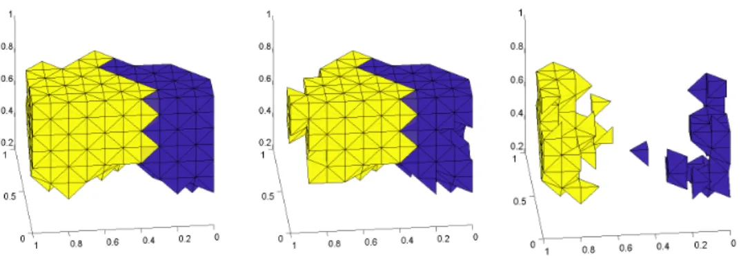
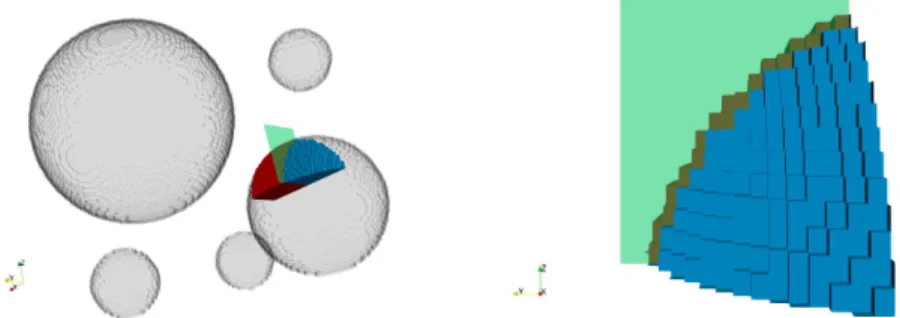
the corresponding eigenvectors vXij to automatically design the coarse space. New
241
coarse components then enforce the constraint (BD,XijSijPDijwXij)TBXijvXij = 0 in
242
each iteration, e.g., with projector preconditioning or transformation of basis. When
243
enforcing these constraints for all faces and edges between subdomains, that do not
244
share a face, we obtain the condition number estimate:
245
(2.13) κ(M−1K)≤4 max{NF, NEME}2T OL;
246
see [33] for the proof. Here, we denote by NF the maximum number of faces of a
247
subdomain, by NE the maximum number of edges of a subdomain, and byME the
248
maximum multiplicity of an edge. The condition number bound thus only depends
249
on geometrical constants of the domain decomposition and, in particular, not on the
250
contrast of the coefficient function. The choice of the tolerance value is user-dependent
251
and should be selected with reference to the spectral gap of the eigenvalues of the
252
preconditioned solver; see also [28].
253
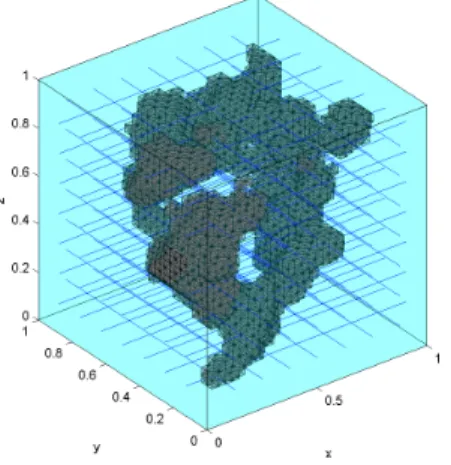
Let us note that the first rigorous proof for the condition number bound was given
254
in [42] for two dimensions and was extendend to three dimensions in [33] with the
255
additional use of edge eigenvalue problems. In [54,55] a condition number indicator
256
was presented for the first time, both for two and three dimensions.
257
2.4. Frugal constraints. As in [24] for the two-dimensional case, we here also
258
consider frugal constraints [23] on certain faces. Frugal constraints build a coarse
259
space which is robust for many diffusion or elasticity problems with jumps in the
260
coefficient function, and the setup of the frugal coarse space is rather cheap compared
261
with the setup of adaptive coarse spaces. This is due to the absence of any local
262
...
...
...
. . . . . . . . . . . .
...
...
Input layer
Hidden layers
Output layer
Fig. 1.Structure of a dense feed forward neural network with several hidden layers.
eigenvalue problems in the computation of the constraints; see [23] for a detailed dis-
263
cussion of frugal constraints. Let us remark that, for each face or edge, a single frugal
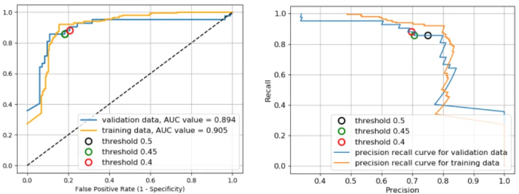
264
constraint can be computed in case of a diffusion problem, but up to six in case of a
265
linear elasticity problem. Nevertheless, for many coefficient distributions, using fru-
266
gal constraints exclusively is not sufficient to obtain robustness, and hence, the frugal
267
coarse space has to be enriched by additional adaptive constraints on some specific
268
faces and/or edges. The combination of both coarse spaces, i.e., the adaptive and the
269
frugal coarse space, and how we can exploit the benefits of both approaches using ma-
270
chine learning in the ML-FETI-DP approach, is elaborated later; cf. subsections 3.3
271
and4.3.
272
3. Selecting necessary eigenvalue problems using machine learning.
273
Here, we extend our approach from [24] to three-dimensional problems. In [24], we
274
have used machine learning techniques to predict which eigenvalue problems are nec-
275
essary for robustness of highly heterogeneous two-dimensional linear diffusion and
276
elasticity problems. This approach is based on the observation that, for many re-
277
alistic problems with highly heterogeneous coefficient distributions, a large share of
278
the eigenvalue problems will not yield large eigenvalues µij > T OL. In particular,
279
the number of large eigenvalues that correspond to an equivalence class Xij can be
280
attributed to the local part of the coefficient function in the adjacent subdomains.
281
Hence, in two dimensions, we used a sampling procedure, to construct, for each edge,
282
an image representation of the coefficient function in the two adjacent subdomains;
283
cf. [24, Sect. 3.1] and Figure 2(left). By ‘sampling procedure’, we understand a spe-
284
cific sequence of evaluations of the coefficient function. Using the resulting image
285
representation as input, a machine learning model was trained to classify whether the
286
corresponding eigenvalue problems yield a large eigenvalue or not. Then, only those
287
eigenvalue problems that are classified as necessary are solved. As already mentioned
288
in the introduction, we denote this hybrid algorithm which combines the adaptive
289
FETI-DP algorithm and a machine learning model as ML-FETI-DP. As an extension
290
to this binary classification, we also introduced a three-class model, which reduces the
291
number of computed eigenvalues even further by additionally using frugal constraints;
292
cf. [23], [24, Sect. 3.3], as well assubsections 2.4and3.3.
293
As described in subsection 2.3.2, edge as well as face eigenvalue problems have
294
to be solved for robustness in three dimensions. However, the edges typically only
295
possess a relatively small number of nodes, and hence, the corresponding eigenvalue
296
problems are rather small; cf. [21]. Therefore, in our three-dimensional approach,
297
we restrict ourselves to the identification of necessary face eigenvalue problems and
298
solve all eigenvalue problems for edges which belong to more than three subdomains.
299
Note that, for unstructured domain decompositions, these edges are rather rare. As
300
in the two-dimensional case, we will additionally consider a three-class approach;
301
cf. subsection 3.3. As input for the machine learning model, we now sample from
302
the three-dimensional coefficient function creating a three-dimensional image repre-
303
sentation; seesubsection 3.1 and Figure 2 (left). This step is significantly extended
304
compared to the two-dimensional case.
305
The eigenvalue classification problem in our approach is essentially an image clas-
306
sification task. Therefore, as in [24], we will employ neural networks, which have been
307
proven to be powerful models for image classification. In general, classification is a
308
task of supervised machine learning. Supervised learning models approximate the
309
nonlinear functional relationship between input and output data F : I → O, with
310
the input space I being a product of R, N, and boolean vector spaces. For classifi-
311
cation problems, as considered here, the output space is typically anNvector space.
312
A detailed description of supervised learning and feedforward neural networks (or
313
multilayer perceptrons, respectively), can, e.g., be found in [17]. Here, we will use
314
dense neural networks, which means that each neuron in a given layer is generally
315
connected with all neurons in the previous layer; cf. Figure 1 for a visualization of
316
a dense feedforward neural network. However, to further improve the generalization
317
properties for our neural network, we use dropout layers with a dropout rate of 20%;
318
see also [24]. Let us note that analogously to [24], we choose the ReLU (Rectified
319
Linear Unit) function [29,56,16] as our activation α(x) in all our numerical experi-
320
ments, which is defined byα(x) = max{0, x}.The training and validation procedure
321
for the neural network model is described in subsection 3.2 and first results on the
322
training and validation data are presented insubsection 3.4.
323
For a complete description of the employed machine learning framework, please
324
refer to [24, Sec. 3] and the references therein.
325
3.1. Data preprocessing. In analogy to [24], we aim to train and test our
326
neural network for both regular domain decompositions as well as for domain decom-
327
positions obtained from the graph partitioning software METIS [30]. We will observe
328
that extending our methods introduced in [24] from two dimensions to three dimen-
329
sions causes additional challenges and additional effort is needed preprocessing the
330
input data for our machine learning model. The preprocessing of input data is at the
331
core of our hybrid ML-FETI-DP algorithm. Hence, the preprocessing of the three-
332
dimensional input data is one of the main novelties compared to the two-dimensional
333
case. Generally, the sampling should cover all elements in a neighborhood of the
334
respective interface component. Therefore, in order to prevent an incorrect or incom-
335
plete picture of the material distribution resulting from gaps in the sampling grid, a
336
smoothing procedure for irregular edges, in two dimensions, or irregular faces, in three
337
dimensions, is necessary; see [24, Fig.4] for a graphical representation of the smooth-
338
ing procedure in two dimensions. Moreover, an additional challenge in the sampling
339
procedure for irregular faces, such as faces obtained via METIS (METIS faces), with
340
an arbitrary orientation in the three-dimensional space, arises. In particular, a con-
341
sistent ordering of the sampling points is neither a priori given nor obvious. More
342
precisely, there is no natural ordering of a grid of points on an irregular face, such as
343
going from the lower left corner to the upper right corner. A consistent ordering of
344
the sampling points is, however, essential when using them as input data to train a
345
neural network. In particular, since neural networks rely on input data with a fixed
346
structure, an important requirement of our data preprocessing is to provide samples
347
sampling order
i1 i2 . . . iN
i2N+1i2N+2. . . i3N
iN+1iN+2 . . . i2N
i3N+1i3N+2. . . i4N
eij
Fig. 2. Left: Visualization of the ordering of the sampling points in 2D (red) for a straight edge (blue). Figure from [24, Fig. 3]. Right:Visualization of the computed sampling points in 3D (red) for a regular face (blue) between two neighboring subdomains. The different shades correspond to increasing distance of the sampling points to the face and therefore to a higher numbering of the sampling points.
of the coefficient distribution with a consistent spatial structure in relation to each
348
face in our domain decomposition, even though the faces may vary in their location,
349
orientation, and shape. In this approach, some sampling points may lay outside the
350
two subdomains adjacent to a face. We encode these points using a specific dummy
351
value which differs clearly from all true coefficient values. Since all coefficient values
352
are positive, we encode sampling points outside the adjacent subdomains by the value
353
−1. This is essential to ensure that we always generate input data of a fixed length
354
for the neural network; see also [24].
355
3.1.1. Sampling procedure for regular faces. In case of regular faces, the
356
procedure is fairly similar to the approach for straight edges in a two-dimensional
357
domain decomposition; see [24]. Basically, we compute a tensor product sampling
358
grid by sampling in both tangential directions of a face as well as in the direction
359
orthogonal to the face. This results in a box-shaped structure of the sampling points
360
in both neighboring subdomains of the face; see also Figure 2 (right). A required
361
consistent ordering of the sampling points is provided by passing through the sampling
362
points ’layer by layer’ with growing distance relative to the face.
363
3.1.2. Sampling procedure for METIS faces. Our sampling procedure for
364
METIS faces consists of two essential steps. First, we construct a consistently ordered
365
two-dimensional auxiliary grid on a planar projection of each face. Second, we extrude
366
this auxiliary grid into the two adjacent subdomains of the face. The resulting three-
367
dimensional sampling grid has both a fixed size and a consistent ordering for all faces.
368
Sampling points which do not lie on the face or within the two adjacent subdomains
369
are encoded using the dummy value−1.
370
First step – Construction of a consistently ordered auxiliary grid for METIS faces.
371
In order to construct the auxiliary grid for a METIS face, we first compute a projection
372
of the original face represented in the three-dimensional Euclidean space onto an
373
appropriate two-dimensional plane. In particular, we project a given METIS face onto
374
a two-dimensional plane, such that we obtain a consistently sorted grid covering the
375
face. This grid is induced by a tensor product grid on the two-dimensional projection
376
plane. Note that since we use tetrahedral finite elements in three dimensions, each
377
METIS face is naturally decomposed into triangles. Due to the projection from three
378
dimensions to two dimensions, elements, i.e., triangles of the face, can be degraded or
379
deformed, i.e., they can have a large aspect ratio. We can also obtain flipped triangles;
380
seeFigure 3for an example where both cases occur. Hence, we have to regularize the
381
two-dimensional projection of the face before constructing the sampling grid.
382
To obtain a well-shaped projection of the face which is appropriate for our pur- pose, we numerically solve an optimization problem with respect to the two-dimensio- nal projection of the face. More precisely, the objective functions of the optimization problem are carefully designed such that flipped triangles (phase 1) as well as sharp- angled triangles (phase 2) are prevented:
minx
X
Tj
λ1·e−λ2·det(Tj(x))+λreg· kd(x)k22 (phase 1) and
minx
X
Tj
lpj2(x) +lqj2(x)
2·Aj(x) (phase 2).
Here, we denote by xthe coordinate vector of all corner points of all triangles of a
383
given face after projection onto the two-dimensional plane, by Aj(x) the area of a
384
given triangleTj(x), and bylpj(x), lqj(x) the lengths of two of its edges. Byd(x) we
385
denote the displacement vector containing the displacements of all pointsxfrom the
386
initial state prior to the optimization process. Furthermore, we denote by det(Tj(x))
387
the determinant of the transformation matrix which belongs to the affine mapping
388
from the unit triangle, i.e., the triangle with the corner points (0,0),(1,0), and (0,1),
389
to a given triangleTj(x). We also introduce scalar weighting factorsλ1, λ2, andλreg 390
to control the ratio of the different terms within the objective functions. The concrete
391
values for these weights were chosen heuristically and for all our computations, we
392
used the valuesλ1= 1, λ2= 50, andλreg= 10.
393
Let us briefly motivate our objective functions in more details. Prior to the
394
optimization of phase 1, we locally reorder the triangle corners, such that det(Tj(x))
395
is negative for all flipped triangles. In order to do so, we start with one triangle and
396
define it either as flipped or non-flipped. Then, we go through the remaining triangles
397
of the projected face and classify them based on the following equivalence relation:
398
two adjacent triangles are equivalent if and only if they do not overlap. Depending on
399
the label of the initial triangle, we obtain two values for the objective function of phase
400
1, and we choose our classification into flipped and non-flipped triangles such that we
401
start with the lower value. After this, flipped triangles can always be identified by a
402
negative determinant of the respective transformation matrix. Therefore, we explicitly
403
penalize such negative determinants in phase 1 of our optimization by minimizing the
404
factorsλ1·e−λ2·det(Tj(x)). Note that we also add the regularization termλreg· kd(x)k22
405
to the objective function to prevent that the projection can be arbitrarily shifted
406
or rotated in the given plane. In phase 2, we minimize the sum of all fractions
407
lpj2(x)+lqj2(x)
2·Aj(x) . This specific fraction is inspired by geometrical arguments; see also [15,
408
Sect. 4]. It is minimized to obtain equilateral triangles, i.e., a high value in this
409
fraction corresponds to a triangle with large aspect ratio. The fraction may actually
410
be infinity if Aj(x) = 0. This may happen if a triangle is initially projected onto
411
a straight line. However, in the first optimization phase, small areas are penalized
412
in terms of the determinant, such that we do not obtain values close to zero in the
413
second phase.
414
We start the optimization procedure with the initial projection onto the plane
415
x = 0, y = 0, or z = 0 that results in the lowest objective value when adding
416
Fig. 3. Left: Example of a typical METIS face in the three-dimensional space (blue triangles) and its corresponding projection onto the two-dimensional plane z = 0 (green triangles). Right: Due to the projection, we obtain both flipped triangles, which are marked in grey with red edges, and degraded triangles with a large aspect ratio, from which one is marked in blue. Let us remark that the different shades of green are only introduced for visualization purpose and do not have any physical meaning, e.g., different coefficients.
the objective functions of phase 1 and phase 2. Then, we use the gradient descent
417
algorithm as an iterative solver and optimize, i.e., minimize, alternating in succession
418
the two aforementioned objective functions. The optimization procedure is stopped if
419
the norm of the relative change of the coordinate vector of the triangles with respect
420
to the prior iteration is below a factor of 1e−6 in both phases. Please see Figure 4
421
and Figure 5 for an example of the different steps of the optimization procedure in
422
phase 1 and phase 2, respectively, for an exemplary METIS face consisting of ten
423
triangles. Let us note that for all tested faces insection 4the optimization procedure
424
did always converge in phase 1 and phase 2, respectively, before the maximum number
425
of iterations was reached, which we set to 500. Additionally, in almost all cases, only
426
optimizing twice in phase 1 and once in phase 2 - alternating in succession - was
427
necessary to obtain an appropriate projection of a given METIS face.
428
As the next step, we construct the smallest possible two-dimensional tensor
429
product grid aligned with the coordinate axes covering the obtained optimized two-
430
dimensional projection of the face; see also Figure 6 (left) for an example. Let us
431
remark that this grid has a natural ordering of the grid points starting in the lower
432
left corner and proceeding row by row to the upper right corner. We then make use
433
of barycentric coordinates to map the grid, together with the corresponding ordering,
434
back into the original triangles in the three-dimensional space. Based on the ordering
435
of the grid points in two dimensions, we can now establish a natural ordering of the
436
points in three dimension; see alsoFigure 6(right).
437
Let us summarize the complete process to obtain the auxiliary grid points for
438
each triangle of a specific face with a consistent ordering. First, we project the face
439
from the three-dimensional space (Figure 3(left: blue face)) onto a two-dimensional
440
plane (Figure 3(left: green face)). Second, we remove all flipped triangles (phase 1)
441
and optimize the shape of all triangles (phase 2) of the projected face in an iterative
442
optimization process; see Figures 4 and 5. Finally, we cover this optimized face by
443
a two-dimensional tensor product grid with a natural ordering (Figure 6 (left)) and
444
project these points back to the original face in three dimensions (Figure 6 (right)).
445
Therefore, local barycentric coordinates can be used.
446
Let us note that, in our numerical experiments in section 4, this procedure was
447
Fig. 4.Visualization of the optimization process of the original projection in two dimen- sions inphase 1after 0, 20, 30, 50, 100 and 150 iteration steps (from upper left to lower right).
Fig. 5.Visualization of the optimization process of the original projection in two dimen- sions in phase 2 after 0, 10, 30, 50, 70 and 100 iteration steps (from upper left to lower right). Let us remark that the initial state here is the same as the final state fromFigure 4.
always successful. However, in general, there may be rare cases where our optimization
448
does not converge to an acceptable two-dimensional triangulation. For instance, it is
449
possible that a subdomain is completely enclosed by another subdomain, such that
450
the face between the two subdomains is actually the complete boundary of the interior
451
subdomain. In this case, we cannot remove all flipped triangles without changing the
452
structure of the face. If we detect that our optimization does not converge to an
453
acceptable solution, we can still proceed in the two following ways: either we mark
454
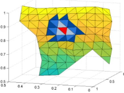
Fig. 6. Left: Two-dimensional projection of the original face (depicted on the right) after both optimization phases have been carried out; the optimized projection is covered by a regular grid with natural ordering; same face as in the last picture ofFigure 5. Right: Original face in three dimensions with corresponding grid points; numbers are obtained by a projection from two dimensions (left) back to three dimensions using barycentric coordinates.
the eigenvalue problem corresponding to the face as necessary, or we split the face into
455
smaller faces and consider each of the smaller faces separately in our ML-FETI-DP
456
algorithm.
457
Second step – Extrusion of the auxiliary grid into three dimensions. Starting
458
from the ordered auxiliary points on the face, we can now build a three-dimensional
459
sampling grid. For this purpose, for each of the auxiliary points on the face, we first
460
define asampling direction vectorpointing into one of the two adjacent subdomains.
461
Second, we extrude the two-dimensional auxiliary grid on the actual METIS face into
462
the two neighboring subdomains along the sampling directions, resulting in a three-
463
dimensional sampling grid. Note that the first layer of sampling nodes does not lie
464
on the face itself but next to it; cf. Figure 2. Moreover, we neglect all points of the
465
auxiliary grid, which are outside the METIS face, and encode all corresponding points
466
in the three-dimensional sampling grid by the dummy value−1. Similar as for edges
467
obtained by a two-dimensional METIS decomposition, choosing the normal vectors
468
of the triangles as sampling direction vectors in the extrusion process leads to gaps
469
in the three-dimensional sampling grid close to the face; see also [24, Sec. 3.1, Fig.
470
4] for a two-dimensional graphical representation. This is caused by the fact that,
471
in general, METIS faces are not smooth. As we have already shown for edges in the
472
two-dimensional case, the neighborhood of an interface component will be the most
473
important for the decision if adaptive constraints are necessary or not and therefore
474
the aforementioned gaps have to be minimized; see [25]. To avoid these gaps and thus
475
to obtain sampling points in most finite elements close to the face, we suggest the use
476
of sampling directions obtained by a moving average iteration over the normal vectors
477
of the face. In some sense, this can be interpreted as a smoothing of the face or, more
478
precisely, the field of normal vectors on the face.
479
The following procedure turned out to be the most appropriate for our purposes
480
in the sense that, on average, for each face and each neighboring subdomain, it results
481
in the highest number of sampled elements relative to the overall number of elements
482
in the subdomain. Here, we first uniformly refine all triangles of a given METIS face
483
once by subdividing each triangle of the face into four new regular triangles. For
484
Fig. 7.Visualization of the moving average procedure to obtain the sampling direction vectors for the extrusion of the auxiliary grid. For the red triangle, all grey, light blue and dark blue triangles are considered recursively as grouped by colors for a moving average with a window length of 3.
each of the resulting finer triangles, we compute the normal vector originating in its
485
centroid. We then use the normal vectors of the refined triangulation to compute a
486
single sampling direction for each triangle of the original triangulation of the face. For
487
this purpose, we first ’smooth’ the field of normal vectors of the refined triangulation
488
by using a component-wise moving average, applied twice recursively with a fixed
489
window length of 3. Subsequently, by computing the average of the resulting normal
490
vectors of all four related finer triangles we finally obtain the sampling direction of
491
the original triangles. Then, we use the same sampling direction for all points of the
492
auxiliary grid which are located in the same triangle.
493
Let us briefly describe the moving average approach and the meaning of the
494
window length in more details. For each triangle of the refined face, one after another,
495
we replace the normal vector by a component-wise average of the normal vector itself
496
and the normal vectors of certain surrounding triangles. The triangles considered in
497
the averaging process are aggregated recursively as follows. In a first step, for a given
498
triangle, we add all neighboring triangles that share an edge with the given triangle
499
to obtain a patch with a window length of 1. Recursively, for an increasing window
500
length, we add all triangles that share an edge with a triangle that has been selected
501
in the previous step. Please see also Figure 7 for an exemplary visualization of all
502
considered triangles for a moving average with the window length of 3.
503
Finally, we use the obtained sampling directions to compute the final three-
504
dimensional sampling grid in the two neighboring subdomains of the face. InFigure 8,
505
we visualize all sampled (middle) and non-sampled (right) finite elements using the
506
described procedure for an exemplary METIS face; we call a finite element “sampled”
507
if it contains at least one sampling point. We can observe that, especially in the close
508
neighborhood of the face, we obtain sampling points in almost all finite elements.
509
As final input for our neural network, we use a vector containing evaluations of
510
the coefficient functionρor the Young modulusE, respectively, for all points in the
511
sampling grid.
512
3.2. Training and validation phase. For the training and validation of the
513
neural network, we use a data set containing approximately 3 000 configurations of
514
pairs of coefficient functions and subdomain geometries for two subdomains sharing a
515
face. To obtain the output data, i.e., the correct classification labels, for the training
516
of the neural network, we solve the eigenvalue problem described insubsection 2.3.2
517
for each of these configuration. Note that the correct classification label for a specific
518
face does not only depend on the geometry and the coefficient distribution but also
519
Fig. 8. Visualization of a METIS face between two neighboring subdomains (left) and all sampled(middle)and non-sampled(right)FE’s when using the described sampling procedure.
on the underlying PDE. Therefore, we will use the same configurations for diffusion
520
and elasticity problems but compute the correct classification labels separately.
521
In [24], for the two-dimensional case, we used only two edge geometries, i.e., a
522
regular edge and an edge with a single jag, and combined them with a set of carefully
523
designed coefficient distributions, resulting in a total of 4 500 configurations; in [22],
524
this data set based on manually designed coefficient distributions was also referred to
525
as ‘smart data’. Since both the domain decomposition and the coefficient distribution
526
may be more complex in three dimensions compared to two dimensions, we use a
527
different approach for the generation of our training and validation data. In particular,
528
we consider six different meshes resulting from regular domain decompositions of the
529
unit cube into 4×4×4 = 64 or 6×6×6 = 216 subdomains of sizeH/h = 6,7,8.
530
For each of these meshes, we generate 30 different randomly generated coefficient
531
distributions based on the approach discussed in [22]. More precisely, we control the
532
ratio of high vs. low coefficient voxels and impose some light geometrical structure.
533
In particular, we build connected stripes of high coefficient with a certain length in
534
x, y, or z direction, and additionally combine them by a pairwise superimposition;
535
cf. [22] for a more detailed description for the two-dimensional case andFigure 9for
536
an exemplary coefficient distribution in three dimensions. In analogy to [22], we refer
537
to this set of coefficient functions asrandom data.
538
For each combination of mesh and coefficient distribution, we now consider the
539
aforementioned regular domain decomposition as well as a corresponding irregular do-
540
main decomposition into 64 or 216 subdomains, respectively, obtained using the graph
541
partitioning software METIS [30]. Finally, we consider the eigenvalue problems cor-
542
responding to all resulting faces combined with the different coefficient distributions.
543
As mentioned before, we obtain a total of approximately 3 000 configurations.
544
Note that, in general, using a smaller number of METIS subdomains, we obtained
545
face geometries which resulted in worse generalization properties of our neural net-
546
works. Moreover, in contrast to the two-dimensional case, where we needed at least
547
4 500 configurations, we are here able to obtain very good results for total of only
548
roughly 3 000 configurations. This is likely due to the much smaller numbers of finite
549
elements per subdomain used, compared to our two-dimensional experiments in [24].
550
For the sampling, we select 22 points in both of the two tangential directions of
551
the auxiliary grid of a face and 22 points in orthogonal direction for each of the two
552
adjacent subdomains; hence, we obtain approximately two sampling points in each
553
finite element when using a subdomain size ofH/h= 10.
554
Fig. 9.Example of a randomly distributed coefficient function in the unit cube obtained by using the same randomly generated coefficient for a horizontal or vertical beam of a maximum length of 4 finite element voxels. The grey voxels correspond to a high coefficient and we have a low coeffient of1otherwise. Visualization for2×2×2subdomains andH/h= 5.
Fig. 10. ROC curve and precision-recall plot for the optimal model obtained by a grid search.
We define precision as true positives divided by (true positives+false positives), and recall as true positives divided by (true positives+false negatives). The thresholds used insection 4are indicated as circles.
As in [24], we train the neural network using the Adam (Adaptive moments) [32]
555
optimizer, a variant of the Stochastic Gradient Descent (SGD) method with adaptive
556
learning rate. The hyper parameters for the training process and the neural network
557
architecture are again chosen based on a grid search with cross-validation. More
558
precisely, we compare the training and generalization properties of different neural
559
networks for several random splittings of our entire data set into 80 % training and
560
20 % validation data; cf. [24] for details on the hyper parameter search space and finally
561
chosen set of hyper parameters. The Receiver Operating Characteristic (ROC) curve
562
and a precision-recall plot of the neural network with optimal hyper parameters are
563
shown inFigure 10. Let us note that we use the same neural network for both, regular
564
and METIS decompositions, in our numerical experiments.
565
3.3. Extension to three-class classification using frugal face constraints.
566
As described insubsection 2.4, we can replace the adaptive constraints by less costly
567
frugal constraints on faces, where only a single constraint (in case of a stationary
568
diffusion problem) or less than or equal to six constraints (in case of linear elasticity)
569
are necessary. Please see [23] for a detailed description of the resulting frugal con-
570