Technical Report Series Center for Data and Simulation Science

Technical Report Series

Center for Data and Simulation Science

Alexander Heinlein, Christian Hochmuth, Axel Klawonn

Reduced Dimension GDSW Coarse Spaces for Monolithic Schwarz Domain Decomposition Methods for Incompressible Fluid Flow Problems

Technical Report ID: CDS-2019-12

Available at http://kups.ub.uni-koeln.de/id/eprint/9675

Submitted on May 30, 2019

DOI: xxx/xxxx

ARTICLE TYPE

Reduced Dimension GDSW Coarse Spaces for Monolithic Schwarz Domain Decomposition Methods for Incompressible Fluid Flow Problems

Alexander Heinlein^1,2 | Christian Hochmuth¹ | Axel Klawonn*^1,2

1Department of Mathematics and Computer Science, University of Cologne, Weyertal 86-90, 50931 Köln, Germany

2Center for Data and Simulation Science, University of Cologne, Germany, url: http://www.cds.uni-koeln.de Correspondence

*Axel Klawonn, Department of Mathematics and Computer Science, University of Cologne, Weyertal 86-90, 50931 Köln, Germany. Email:

axel.klawonn@uni-koeln.de Present Address

Weyertal 86-90, 50931 Köln, Germany

Summary

Monolithic preconditioners for incompressible fluid flow problems can significantly improve the convergence speed compared to preconditioners based on incomplete block factorizations. However, the computational costs for the setup and the appli- cation of monolithic preconditioners are typically higher. In this paper, several techniques to further improve the convergence speed as well as the computing time are applied to monolithic two-level Generalized Dryja–Smith–Widlund (GDSW) preconditioners. In particular, reduced dimension GDSW (RGDSW) coarse spaces, restricted and scaled versions of the first level, hybrid and parallel coupling of the levels, and recycling strategies are investigated. Using a combination of all these improvements, for a small time-dependent Navier-Stokes problem on 240 MPI ranks, a reduction of 86 % of the time-to-solution can be obtained. Even without apply- ing recycling strategies, the time-to-solution can be reduced by more than 50 % for a larger steady Stokes problem on 4 608 MPI ranks. For the largest problems with 11 979 MPI ranks the scalability deteriorates drastically for the monolithic GDSW coarse space. On the other hand, using the reduced dimension coarse spaces, good scalability up to 11 979 MPI ranks, which corresponds to the largest problem configuration fitting on the employed supercomputer, could be achieved.

KEYWORDS:

domain decomposition, overlapping Schwarz, reduced dimension coarse space, GDSW, algebraic precon- ditioner, parallel computing, incompressible fluids, Stokes, Navier-Stokes

1 INTRODUCTION

We discretize the underlying partial differential equations of incompressible fluid flow problems with mixed finite elements. Fine discretizations of the Stokes and Navier-Stokes equations using such mixed finite elements result in large and ill-conditioned indefinite linear systems. In addition to the required inf-sup conditions for finite element discretizations of such saddle point problems, special care has to be taken when constructing preconditioners for the discrete problem. The block structure and the coupling blocks have to be handled appropriately to guarantee fast convergence of iterative methods.

We consider monolithic two-level preconditioners with Generalized Dryja–Smith–Widlund (GDSW) coarse spaces for incom- pressible fluid flow problems introduced in¹. GDSW coarse spaces were originally introduced in^2,3for linear second and fourth order elliptic partial differential equations. For these elliptic problems, the GDSW coarse basis functions are energy minimal

extensions representing the null space of the elliptic operator. In¹, this concept was extended to coarse basis functions which are saddle point extensions of the null spaces of velocity and pressure of the indefinite saddle point operator. One significant advan- tage of GDSW coarse spaces is that they can be applied to arbitrary geometries and domain decompositions, whereas the use of classical Lagrangian coarse basis functions requires a coarse triangulation. In particular, for unstructured meshes and domain decompositions, a coarse triangulation is typically not available. Our monolithic GDSW approach is inspired by the work of Klawonn and Pavarino^4,5, who introduced monolithic two-level Schwarz preconditioners for saddle point problems for the first time; however, the methods presented therein are less practical for realistic problems since Lagrangian coarse spaces were used.

Results without algorithmic details for monolithic GDSW coarse spaces were presented by Clark Dohrmann at a workshop on adaptive finite elements and domain decomposition methods; cf.⁶.

An overview of different solution strategies for saddle point problems is given in⁷. Exact and inexact Uzawa algorithms are among the first methods for the iterative solution of those saddle point problems; cf.^8,9. For these algorithms velocity and pressure are decoupled and solved in a segregated approach. Another approach, which is based on the decoupling of the physical variables, is SIMPLE (Semi-Implicit Method for Pressure Linked Equations); cf.¹⁰. Furthermore, preconditioned iterative solvers such as the Generalized Minimum Residual Method (GMRES) and its variants or the Conjugare Residual method are widely used.

Block-diagonal and -triangular preconditioners, based on block factorizations, have been developed in11,12,13,5,14,15,16,17,18. More advanced block preconditioners are the PCD (Pressure Convection-Diffusion) preconditioner^19,20,21, the LSC (Least-Squares Commutator) preconditioner²², Yosida’s method^23,24, the Relaxed Dimensional Factorization (RDF) preconditioner²⁵and the Dimensional Splitting (DS) preconditioner^26,27. Early studies of domain decomposition methods for the Stokes problem were conducted in²⁸. Domain decomposition based Schwarz preconditioners for Stokes and mixed elasticity problems have already been used for the approximation of the inverse matrices of blocks in⁵and as monolithic preconditioners in4,29,30,31,32. Alternative solvers for saddle point problems are, e.g., multigrid methods; cf.^33,34,35.

In order to improve the parallel performance of monolithic GDSW preconditioners, we will reduce the dimension of the coarse spaces following the work by Dohrmann and Widlund³⁶ on reduced dimension GDSW (RGDSW) coarse spaces; the smaller dimension typically results in a significantly better parallel performance; cf.³⁷. Other earlier approaches to reduce the dimen- sion of GDSW coarse spaces can be found in, e.g.,^38,39. Moreover, we will consider restricted and scaled Schwarz operators, introduced by Cai and Sarkis⁴⁰, in the first level of our monolithic preconditioners. Furthermore, we employ two alternative strategies to improve the additive and sequential coupling of the two levels which was used in¹: multiplicative but sequential coupling of the levels and additive coupling combined with the concurrent computation of the levels. Finally, for nonlinear or time-dependent problems, we will employ different recycling strategies ranging from the re-use of symbolic factorizations of the local overlapping and nonoverlapping matrices to the complete re-use of the coarse basis and matrix. As we will show, recycling of the coarse basis functions can eliminate the drawback of the expensive setup phase of GDSW coarse spaces.

The parallel implementation employed in our numerical simulations is based on our parallel implementation of monolithic two-level preconditioners described in^1,41,42. The implementation is available in theFROSchframework⁴³as a part of theShyLU package in Trilinos⁴⁴.

This paper is structured as follows. In section 2 we introduce as model problems variational formulations of steady and time- dependent incompressible fluid flow problems. Next, in section 3 we state the space and time discretizations of the underlying partial differential equations. We describe the construction of our monolithic two-level Schwarz preconditioner with classical GDSW and reduced dimension GDSW coarse spaces in section 4. We first display different variants of a monolithic one level method and continue with the introduction of reduced coarse spaces. We conclude this section with a presentation of coupling strategies of the first and the second level. Numerical studies for the preconditioners and the considered improvements are presented in section 5.

2 SADDLE POINT PROBLEMS

We construct preconditioners for incompressible fluid flow problems involving the Stokes and Navier-Stokes equations. Our method can be constructed for two dimensional as well as for three dimensional model problems. Here, we concentrate on the three-dimensional case of⌦œR³being a polyhedral domain.

2.1 Stokes equations

)⌦wall )⌦wall

)⌦in )⌦out

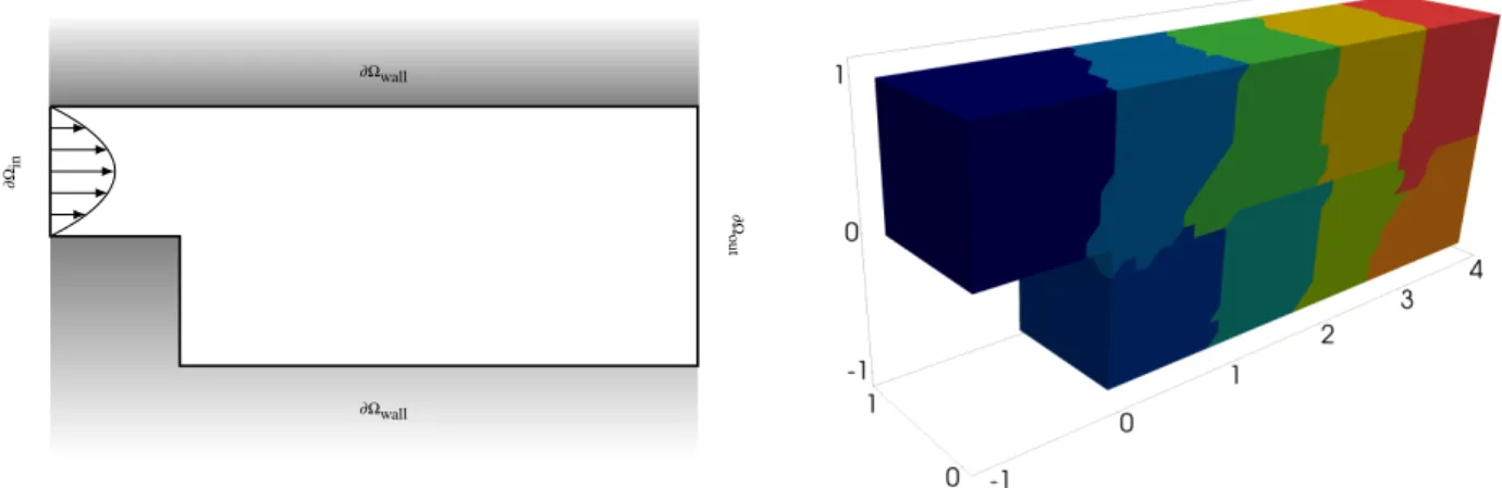
FIGURE 1Cross-section (left) and unstructured domain decomposition into nine subdomains of the three-dimensional back- ward facing step geometry (right). The Dirichlet boundary)⌦_Dconsists of the inlet)⌦_inand the walls)⌦_wall, the outlet)⌦_out is the Neumann boundary)⌦_N; see section 2.1 for the resulting streamline solution of a Navier-Stokes problem.

FIGURE 2Streamline solution of a three-dimensional backward facing step Navier-Stokes problem.

First, we will consider a linear model problem which is given by the Stokes equations. We seek to determine the velocity uÀV_g:= {vÀ(H¹(⌦))³:v_)⌦D =g}and the pressurepÀL²(⌦)of an incompressible fluid with negligible advective forces by solving the variational formulation: find(u,p), such that

 ⌦

(u: (v dx *  

⌦

divv p dx=  _⌦f v dx ≈vÀ(H¹(⌦))³,

* 

⌦

divu q dx = 0 ≈qÀL²(⌦),

with Dirichlet boundary )⌦_D œ )⌦. We consider the three-dimensional Backward Facing Step (BFS) geometry shown in section 2.1; cf.45, Sec. 3.1for the two-dimensional geometry.

The Dirichlet boundary conditions at the inflow and the walls are given by g=<

(16u_maxx2(1*x2)x₃(1*x3),0,0)^T forxÀ)⌦_in, (0,0,0)^T forxÀ)⌦_wall.

tins Qinmm³_s

0.5 1

600

FIGURE 3Inflow rate for the time-dependent Navier-Stokes problem in a coronary artery (left); see figs. 4 and 6 for the cor- responding meshes and flow field. Magnitude of the solution to a three-dimensional Laplacian problem on the inflow boundary (right).

At the outlet, we prescribe do-nothing boundary conditions, i.e., )u

)n *pn= 0 on)⌦_out,

with outward pointing normal vectorn. Furthermore, we choose the source termf í0.

2.2 Navier-Stokes equations

Second, we consider the Navier-Stokes equations, which model the flow of an incompressible Newtonian fluid with kinematic viscosity⌫>0. We seek to determine the velocityu(x,t)ÀV_gand the pressurep(x,t)ÀQ œ L²(⌦)by solving the variational formulation: find(u,p), such that

 ⌦

)u

)tv dx + ⌫ 

⌦

(u: (v dx +  

⌦

(u (u) v dx

*  

⌦

divv p dx= 

⌦

f v dx ≈vÀV₀,

* 

⌦

divu q dx= 0 ≈qÀL²(⌦)

We consider both, time-dependent problems, as well as steady-state Navier-Stokes problems where)u_)t = 0. The presence of the convection termu (u leads to a nonlinear system. In the steady case, we solve the system using Newton’s method, cf.45, Sec. 8.3, whereas, in the time-dependent case, we use a second order extrapolationu^<to linearize the convective part, i.e.,

u (u˘u^< (u.

We choose the source termf í 0and, for the steady-state Navier-Stokes problem, we again use the domain and boundary conditions of the backward facing step Stokes problem. In a dimensionless reformulation of the Navier-Stokes equations, the Reynolds numberRespecifies the relative contributions of convection and diffusion. We obtainRe=L Ñu_⌫with the character- istic length scaleLand maximal inflow velocity Ñu = 1.0. In our numerical tests for the steady Navier-Stokes problem, we set L= 2as the height of the outlet and choose⌫= 0.01; i.e.,Re= 200.

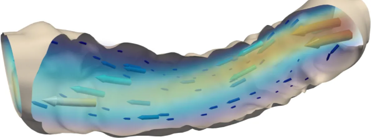
For the time-dependent Navier-Stokes problem, we consider a geometry of a realistic coronary artery; cf. figs. 4 and 6. This geometry was generated by bending a straight coronary artery geometry used for the simulation of stress distributions in the walls of patient-specific atherosclerotic arteries in^46,47.

FIGURE 4Coronary artery volume mesh with 1 032 k tetrahedral elements. Resulting Navier-Stokes systems discretized with P2-P1 Taylor-Hood elements consists of 4.6 million degrees of freedom.

We prescribe a parabolic inflow profile with increasing flow rate for the first0.5s; cf. fig. 3. After a flow rate ofQsteady = 600 mm³_s is reached, we keep the flow rate constant for further 0.5s. Again, we apply no-slip and do-nothing boundary conditions, respectively, at the wall and the outlet of the arterial geometry.

3 FINITE ELEMENT AND TIME DISCRETIZATION

For the spatial discretization of the incompressible fluid flow problems considered here, we use mixed finite elements. Therefore, we first introduce a triangulation⌧_hof⌦with characteristic mesh sizeh, which can be non-uniform. Then, we introduce the conforming discrete piecewise quadratic velocity and piecewise linear pressure spaces

V^h(⌦) = {v_hÀ(C(⌦))^d„V :v_h_T ÀP2≈T À⌧_h}and Q^h(⌦) = {q_hÀC(⌦)„Q:q_h_T ÀP1≈T À⌧_h}, respectively, of Taylor-Hood (P2-P1) mixed finite elements.

The resulting discrete Stokes and linearized steady Navier-Stokes systems have the generic form Ax=4

F B^T B 0

5 4u p 5

=4 f0

5

=b, (1)

withA À R^nùnandx,b À Rⁿ. Moreover, we discretize the time-dependent problem with BDF2 (Backward Differentiation Formula). Thus, we obtain the discrete system

A_m+1x_m+1=b_m+1 with Am+1 = 3

t 4M 0

0 0 5

+

4F_m+1 B^T

B 0

5 and b_m+1 = 1

t 4M 0

0 0 5 0

44 u_m p_m 5

*4 um*1

p_m*1

51 (2)

for timestepm+1.m= 1, ...,M, and constant timestep size t=T_M. The second order extrapolation readsu^< = 2u_m*um*1.

4 TWO-LEVEL OVERLAPPING SCHWARZ PRECONDITIONERS FOR SADDLE POINT PROBLEMS

We solve the discrete saddle point problems eq. (1) or eq. (2) iteratively using a Krylov subspace method. Since the systems become very ill-conditioned for smallh, we need a scalable preconditioner to guarantee fast convergence of the iterative method.

Therefore, we will apply monolithic overlapping Schwarz preconditioners for saddle point problems; cf.^4,5,1. In particular, we will improve the performance of the monolithic preconditioners with GDSW type coarse spaces introduced in¹. In contrast to the

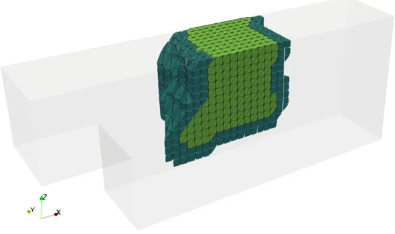
FIGURE 5A nonoverlapping subdomain (light green) of the three-dimensional BFS unstructured decomposition with overlap

= 2h(dark green).

preconditioners described in^4,5, which use Lagrangian coarse spaces, GDSW coarse spaces can be constructed in an algebraic fashion without an additional coarse triangulation. We refer to^1,48 for a detailed description of the parallel implementation of GDSW coarse spaces for elliptic and saddle point problems, respectively.

Let⌦ be decomposed into nonoverlapping subdomains ⌦_i ^N_i=1 with typical diameter H and corresponding overlapping subdomains ⌦^®_i ^N_i=1withklayers of overlap, i.e., =kh. The overlapping subdomains can be constructed from the nonover- lapping subdomains by recursively adding one layer of elements to the subdomains; cf. section 4 for a subdomain with overlap

= 2h. Even if no geometric information is given, this can be performed based on the graph of the matrixA.

Furthermore, let

=$

xÀ(⌦_i„ ⌦_j)‰)⌦_Diëj,1fi,jfN%

(3) be the interface of the nonoverlapping domain decomposition.

We decompose the spacesV^handQ^hinto local spaces

V_i^h=V^h(⌦^®_i)andQ^h_i =Q^h(⌦^®_i),

i = 1, ...,N, respectively, defined on the overlapping subdomains⌦^®_i. This decomposition yields corresponding restriction operators

R_u,i:V^h,ôV_i^hand R_p,i:Q^h ,ôQ^h_i,

i= 1, ...,N. Consequently,R^T_i,uandR^T_i,pare extension operators from local velocity and pressure spaces to the corresponding global spaces.

We combine the restriction operators for velocity and pressure to obtain the corresponding monolithic restriction operators of our global problem eq. (1) or eq. (2) to local overlapping saddle point problems

R_i:V^hùQ^h,ôV_i^hùQ^h_i, i= 1, ...,N, which are of the form

R_i:=4 R_i,u 0

0 R_i,p 5

.

The local saddle point matrices

A_i=R_iAR^T_i,i= 1, ...,N, (4)

are extracted from the global problem matrixAand possess homogeneous Dirichlet boundary conditions for both, velocity and pressure. Therefore, they are always nonsingular. If a zero mean value condition is prescribed for the global problem eq. (1) or eq. (2), also a local zero mean value condition must be satisfied to guarantee numerical scalability; cf.¹.

Then, the monolithic one-level Additive Schwarz (AS) preconditioner can be written as BÇ^*1_AS =…^N

i=1R^T_iA^*1_i R_i.

4.1 Restricted and scaled first level

In many cases, the convergence of the iterative solver can be improved by using restricted or scaled first-level extension oper- ators, resulting in a Restricted Additive Schwarz (RAS) or a Scaled Additive Schwarz (SAS) method, respectively; cf.⁴⁰. Both approaches result from the idea to introduce alternative extension operatorsRÉ^T_i which satisfy

…N i=1

RÉ^T_iR_i1 = 1,

where1ÀRⁿis the vector of ones. The resulting preconditioner reads BÇ^*1_{RAS_SAS} =…^N

i=1

RÉ^T_iA^*1_i R_i.

For the RAS method,RÉ^T_i is obtained from a unique distribution of the degrees of freedom (d.o.f.) among the nonoverlapping subdomains. Therefore,RÉ^T_i can be applied without communication in a parallel implementation of the RAS method.

In contrast, for SAS, the extensionsRÉ^T_i are obtained from theR^T_i by an inverse multiplicity scaling, i.e., RÉ^T_i = diag

H_N

…

i=1R^T_iR_i1 I*1

R^T_i .

Here, the application ofRÉ^T_i requires the same communication as the application ofR^T_i but often improves the convergence of the Schwarz method; cf.⁴⁹.

In the next section, we will describe coarse spaces for two-level overlapping Schwarz methods which are used to guarantee numerical scalability in the case of many subdomains.

4.2 Monolithic GDSW preconditioner

Monolithic two-level additive preconditioners can be written as BÇ^*1_M = A^*1₀ ^T +…^N

i=1R^T_iA^*1_i R_i, (5)

where the matrix of the coarse problem reads

A0 = ^TA (6)

and the columns of the matrix correspond to the coarse basis functions; cf.^4,5,1.

The GDSW preconditioner, which was introduced by Dohrmann, Klawonn, and Widlund in^2,3for certain elliptic problems, is a two-level additive overlapping Schwarz preconditioner with energy minimizing coarse space and exact solvers. In particular, a partition of the domain decomposition interface and discrete harmonic extensions from the interface to the interior d.o.f. are used to construct the coarse basis in an algebraic way.

Here, we concentrate on the construction of GDSW type coarse spaces for Stokes and Navier-Stokes problems of the form (1) or (2); cf.¹. Let the discrete interfaces ^h_uand ^h_pbe the sets of finite element nodes on for the velocity and pressure discretiza- tions; only for equal order discretizations, they typically coincide. The interfaces ^h_u and ^h_p are further divided into connected

components, ^h_u,i,i= 1, ...,M_uand ^h_p,j,j = 1, ...,M_p. For standard GDSW coarse spaces, the connected components ^h_u,iand

hp,jare chosen to be sets of nodes which belong to the same subdomains, i.e., vertices, edges, and faces.

Now, letZbe the null space of the global Neumann matrix,Z_uthe velocity part, andZ ^h_u,ithe restriction ofZ_uto the interface component ^h_u,i. Then, we construct corresponding matrices ^h_u,i, such that their columns form a basis of the spaceZ_u,i. Let R ^h_u,i be the restriction from ^h_u to ^h_u,i, then the interface values of the velocity basis functions read

u=⌧

R^T_u,1 ^h_u,1 ... R^Th u,Mu

hu,Mu . (7)

We construct the interface pressure based basis functions ^h_p accordingly and obtain the interface part of complete monolithic coarse basis

= L

hu 0

0 h

p

M

. (8)

Note that the columns of ^h_u and ^h_p are the restrictions of the null spaces of the Neumann operators corresponding toAand B^T, respectively, to the vertices, edges, and faces. Typically, the null space of the operatorB^T consists of all pressure functions that are constant on⌦. Therefore, the columns of ^h_p are chosen to be the restrictions of the constant function1to the vertices, edges, and faces. For the three-dimensional flow problems considered here, the null spaces ofAandB^T are spanned by

ru,1:=b ff d 10 0 cg

ge, ru,2 :=b ff d 01 0 cg

ge, andru,3 :=b ff d 00 1 cg ge

andrp,1:=⌅ 1⇧

, (9)

respectively. To compute the values in the interior d.o.f., we distinguish between interface ( ) and interior (I) d.o.f. in the discrete system matrix

A=4 A_II A_I A I A

5 .

Each of the four above submatricesA<<is a block matrix of the form eq. (1) or eq. (2). Then, the basis functions of the GDSW coarse space can be written as discrete saddle point extensions of to the interior d.o.f.:

=4

I

5

=4*A^*1_IIA_I 5

. (10)

Note thatA_II= diag^N_i=1(A⁽ⁱ⁾_II)is a block diagonal matrix containing the local matricesA⁽ⁱ⁾_IIfrom the nonoverlapping subdomains.

Its factorization can thus be computed block by block and in parallel. As described in¹, we drop the off-diagonal blocks p,u0

and _u,p0from

=4

u,u0 u,p0

p,u0 p,p0

5

and obtain the coarse basis matrix

=4

u,u0 0 0 _p,p0

5 .

Here, columnsu0andp0belong to velocity and pressure basis functions, respectively. This reduces the costs for the computation of the coarse matrix eq. (6) using an RAP matrix product without worsening the convergence.

4.3 Monolithic reduced dimension GDSW preconditioner

In order to reduce the dimension of our GDSW coarse spaces, we follow^36,1 and introduce monolithic reduced dimension GDSW (RGDSW) coarse spaces. More precisely, we combine the construction described in section 4.2 with a different choice of interface components and interface values.

For the parallel implementation of monolithic RGDSW coarse spaces, we extend our implementation of monolithic GDSW coarse spaces¹ and combine it with the parallel implementation of RGDSW coarse spaces for elliptic problems in FROSch;

cf.³⁷. We refer to these articles for details on the parallel implementation. As in³⁷, we only consider Option 1 and Option 2.2 of the RGDSW variants proposed in³⁶; Option 1 is algebraic and Option 2.2 additionally requires the coordinates of the finite element nodes.

Again, we will concentrate on the construction of the interface values of the velocity basis functions ^h_u; the construction of interface values for pressure basis functions ^h_pis then performed analogously. We denote byS_cuthe index set of all subdomains which share the velocity interface component (i.e., vertex, edge, or face)c_u. Here, we distinguish between velocity and pressure components to allow for nonequal order discretizations or staggered grids. Furthermore, we define a hierarchy of all interface components, where we call a componentc_u,iancestorofc_u,jifS_cu,j œS_cu,i; conversely, we callc_u,ioffspringofc_u,jifS_cu,j –S_cu,i. If a componentc_u,jhas no ancestors, it is classified as acoarse componentand its corresponding basis functions will be part of the RGDSW coarse space. Now, letÉ_u,i^h,i= 1, ...,MÉ_u, be the coarse components of the RGDSW coarse space and

É^h_u,i:= Õ

S_cuœS_Éh

u,i

c_u

the union of the coarse componentÉ_u,i^h and its respective offspring; the É^h_u,i,i= 1, ...,MÉ_u, define an overlapping decomposition of the interface ^h_u.

Similar to the GDSW coarse space, letRÉ^h_u,i be the restriction fromÉ^h_u toÉ^h_u,i. Furthermore, letSÉ^h_u,i ÀR^{ÉhuùÉhu}be a suitable scaling, such that we obtain an interface partition of unity

MÉu

…

i=1SÉ^h_u,iR^T_Éh

u,iRÉ^h_u,i1 = 1_É

u, where1_É

uÀR^Éhuis the vector of ones on the interface. Depending on the choice of the scaling matricesSÉ^h_u,i,i= 1, ...,MÉ_u, we obtain different reduced dimension coarse spaces. Now, we define

RÉÉ^h_u,i :=SÉ^h_u,iRÉ^h_u,i.

Then, the interface values of the velocity basis functions can be written in the same form as for the classical GDSW coarse spaces

É_u=⌧RÉ^T_Éh

u,i É^h_u,1 ... RÉ^T_Éh u,MuÉ É^h

u,MuÉ ;

cf. (7). Here, as in the classical GDSW coarse spaces, the columns of É^h_u,iform a basis of the restriction of the null spaceZ_uto the É^h_u,i, such that the columns of É_uspan the null spaceZ_u.

Now, let us construct the scaling matricesSÉ^h_u,i for variants of the RGDSW coarse space denoted asOption 1andOption 2.2 in³⁶. In Option 1,

sÉ^h_u,i =

T1_ÛÛÛC_cuÛÛÛ ifc_u,i ÀC_cu,

0 otherwise,

withC_cubeing the set of all velocity ancestors of the interface componentsc_u. The corresponding scaling matrices read SÉ^h_u,i = diag⇠

sÉ^h_u,i

⇡.

Another option to define the scaling matrices results from using basis function based on an inverse distance weighting approach; cf.³⁶. In particular, the values of the scaling vectors are chosen as

sÉ^h_u,i = hn ln j

1_d_i(c_u)

≥

cu,jÀCcu

1_dj(cu) ifc_u,iÀC_un,

0 otherwise (11)

andd_i(c_u)is the distance from the componentc_uto the coarse componentc_u,i. This construction is denoted as Option 2.2 in³⁶. It relies on additional geometric information to allow for the computation of the distance between different interface components.

Therefore, it can be regarded as less algebraic compared to Option 1.

The coarse pressure basis functions ^h_p are built analogously. We obtain the monolithic interface values, analogously to eq. (8), and extend them to the interior; cf. eq. (10).

The advantage of the reduced dimension coarse spaces over the classical GDSW coarse spaces is the significantly smaller dimension of the coarse problem. As has been shown numerically in³⁷ for elliptic problems in 3D and structured domain decompositions, RGDSW coarse problems can be smaller by more than 85 %; this typically results in much better parallel scalability.

For results on the improved parallel scalability for incompressible fluid flow problems due to the use of reduced dimension GDSW coarse spaces, see section 5.1.

4.4 Sequential and parallel computation of the levels

In our previous implementation of the two-level additive Schwarz preconditioner eq. (5), the levels are computed in a sequential way; cf.^1,41,42. However, since the coarse problem is typically solved on a small subset of MPI ranks, most of the cores are idle in the mean time. We will tackle this issue by two different approaches, i.e., by multiplicative but sequential coupling of the levels as well as by additive coupling combined with parallel computation of the levels. Both approaches improve the performance of our solver; cf. section 5.3.

Multiplicative Coupling of the Levels

In general, a multiplicative coupling of the levels yields better convergence of the method. In particular, we use the hybrid preconditioner

BÇ^*1_hybrid= (I*P0)BÇ^*1_AS(I*P0)^T + A^*1₀ ^T,with P0= A^*1₀ ^TA;

cf.50, Sec. 2.5.2. In a projected Krylov method with suitable initial vectorx₀ = A^*1₀ ^Tb, the application of the hybrid precondi- tionerBÇ^*1_hybridrequires only one additional application of the system matirxAcompared to the two-level additive preconditioner BÇ^*1_M. However, due to the multiplicative coupling of the levels, they have to be applied sequentially.

Parallel Computation of the Levels

When an additive coupling of the levels is used, a significant amount of work for the construction and the application of the levels can be performed in parallel. Therefore, we split the MPI ranks among the levels. For a fixed total number of MPI ranks, this decreases the number of subdomains and increases the size of the overlapping subdomains; since the number of MPI ranks used for the coarse problem is typically small, the size of the overlapping subdomains is increased only slightly. In addition to that, the coarse basis functions and the coarse matrixA0are computed on the MPI ranks assigned to the first level. However, the factorizations and forward-backward solves of the local overlapping and the coarse problems can be computed in parallel.

We refer to section 5.3 for results on the speedup for to the above described coupling strategies compared to the sequential additive coupling in the previous implementation.

5 NUMERICAL RESULTS

In this section, we present numerical results of our parallel implementation of the monolithic (R)GDSW preconditioners pre- sented in the previous sections. Our largest fluid flow problems possess more than 400 million degrees of freedom. All parallel computations were carried out on the magnitUDE supercomputer at University Duisburg-Essen, Germany. A regular node on magnitUDE has 64GB of RAM and 24 cores (Intel Xeon E5-2650v4 12C 2.2GHz), interconnected with Intel Omni-Path switches. Intel compiler version 17.0.1 and IntelMKL2017 were used.

Our software framework is based on Trilinos⁴⁴. In particular, our monolithic preconditioners are implemented within the framework ofFROSch, a subpackage of the Trilinos packageShyLU. We use the GMRES implementation of the Trilinos package Belosand our Trilinos based implementation of the steady Stokes and Navier-Stokes problems as well as the implementation of time-dependent Navier-Stokes problems of LifeV⁵¹; note that all our simulations are performed using the linear algebra frameworkTpetraexcept for the LifeV simulations, which are performed usingEpetrainstead. As a direct solver, we use MUMPS5.1.1^52,53through theAmesos(Epetrabased simulations) or theAmesos2interface (Tpetrabased simulations) from Trilinos; we slightly modified theAmesos2interface to facilitate the reuse of symbolic factorizations. The local overlapping problems are solved in serial mode, whereas the coarse problem is solved in parallel mode. We use the default setting ofFROSch to determine the number of MPI ranks for the exact coarse solves; cf.^41,1. Furthermore, we use one MPI rank per core and one subdomain per MPI rank.

The nonlinear steady-state Navier-Stokes problems are solved using Newton’s method with zero initial guess, which results in the solution of a Stokes problem in the first Newton iteration. The stopping criterion is

Òr⁽_nl^k)Ò_Òr⁽⁰⁾_nlÒ f tolnl, withr⁽_nl^k) being thek-th nonlinear residual. In order to solve the linear tangent problems, we apply right preconditioned GMRES (Generalized minimal residual method)⁵⁴with the stopping criterionÒr^(k)Òf tolÒr⁽⁰⁾Ò, where tol = 10^*6 andtol = 10^*4 are the tolerances for the Stokes and steady-state Navier-Stokes problems, respectively, andr^(k) = b*ABÇ^*1(BxÇ ^(k))is thek-th residual.

Prec. #cores 243 1 125 4 608 11 979

GDSW

#its. 84 116 160 202 setup 14.7 s 19.7 s 36.6 s 73.9 s solve 10.7 s 20.9 s 37.5 s 220.0 s total 25.4 s 40.6 s 74.1 s 293.9 s

RGDSW #its. 128 117 111 110

setup 12.6 s 13.7 s 16.2 s 24.0 s Option 1 solve 14.8 s 15.1 s 21.3 s 36.2 s total 27.4 s 28.8 s 37.5 s 60.2 s

RGDSW #its. 135 131 121 123

setup 12.2 s 12.8 s 15.8 s 22.7 s Option 2.2 solve 15.7 s 16.9 s 17.9 s 39.4 s total 27.9 s 29.7 s 33.7 s 62.2 s

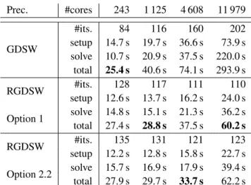
TABLE 1Weak scalability results for different coarse spaces: standard, reduced Option 1 & 2.2 applied to the three-dimensional BFS Stokes,H_h= 10, and = 1h.

In the time-dependent fluid flow simulations for the realistic arterial geometry shown in fig. 4, we apply the inflow boundary condition described in fig. 3 and use a time step length of t= 0.01s and a kinematic viscosity⌫= 3.0 mm²_s. The length of the artery is12 mmand the inflow diameter is approx.2 mm. Here, as for the steady Stokes problems, the linearized systems are solved up to a tolerancetol= 10^*6.

In the following numerical results, we report combined setup times of the first and second level since a distinction is not straightforward for a parallel computation of the levels. The identification of the interface is omited from our setup times.

Furthermore, solve times and total times, which are the sums of the setup and solve times, are reported.

5.1 Comparison of monolithic GDSW and RGDSW coarse spaces

In section 5.1, we compare the performance of different coarse spaces for our monolithic Schwarz preconditioner for the back- ward facing step Stokes problem using structured meshes and domain decompositions in three dimensions. In particular, we consider the GDSW coarse space¹as well as Option 1 and Option 2.2 of the RGDSW coarse space as described in section 4.3.

We obtain a significant reduction of the coarse space dimension when using the RGDSW coarse spaces. For the largest problem with 11 979 subdomains, the dimension of the coarse problem for the standard GDSW coarse space is 305 157 (228 852 velocity and 76 305 pressure basis functions), whereas it is only 40 530 (30 390 velocity and 10 140 pressure basis functions) for the reduced dimension coarse spaces. Thus, compared to the standard GDSW coarse space, the setup of both reduced dimension variants is more than twice as fast for the largest BFS Stokes problem. Surprisingly, iterations counts for the reduced dimension variants are also lower than for the standard GDSW variant for the largest problem. This is typically the opposite for elliptic problems; cf.^36,37. In total, the time to solution for the reduced dimension coarse spaces is lower by more than50 %compared to the standard GDSW coarse space on 4 608 cores. It is also important to note that Option 1 of the RGDSW coarse space performs better than Option 2.2. This is also different compared to elliptic problems; cf.^36,37. However, this is beneficial since Option 1 can be built in an algebraic fashion, whereas Option 2.2 relies on the coordinates of the finite element nodes.

5.2 Restricted and scaled first level variants

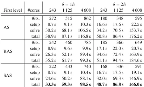
In section 5.2, we present weak scalability results for the three first level variants AS, RAS, and SAS presented in section 4.1 with overlap = 1h,2h. We observe that, even though the iteration counts are higher, an overlap of1hyields the best total computing times for all three different approaches. Furthermore, the iteration counts are always lower for the scaled variant (SAS) compared to the standard (AS) and the restricted (RAS) variants. Therefore, although we save some communication in RAS, SAS performs best for all configurations in this comparison. Surprisingly, the iteration counts for RAS are even higher than for AS for a wider overlap = 2h.

From this point on, we will therefore use SAS with overlap = 1has our default first level.

= 1h = 2h

First level #cores 243 1 125 4 608 243 1 125 4 608

AS

#its. 272 515 862 180 348 595

setup 8.7 s 9.1 s 10.3 s 16.6 s 17.6 s 22.5 s solve 30.2 s 68.1 s 106.5 s 34.2 s 70.5 s 153.7 s total 38.9 s 87.1 s 116.8 s 50.8 s 86.4 s 176.2 s RAS

#its. 242 460 785 185 366 649

setup 8.9 s 9.6 s 9.9 s 17.1 s 22.0 s 20.7 s solve 26.3 s 52.1 s 89.4 s 34.6 s 72.4 s 163.9 s total 35.2 s 61.7 s 99.3 s 51.1 s 94.4 s 184.6 s SAS

#its. 222 433 740 168 336 591

setup 8.7 s 9.1 s 10.4 s 16.7 s 17.5 s 19.1 s solve 24.6 s 50.2 s 88.1 s 32.0 s 69.3 s 146.9 s total 33.3 s 59.3 s 98.5 s 48.7 s 86.8 s 166.0 s

TABLE 2Comparison of the different monolithic one-level Schwarz preconditioners withH_h= 10applied to the BFS Stokes problem: AS, RAS, and SAS; cf. section 4.1.

#cores 243 1 125 4 608 11 979

Coupling #its. 120 114 105 108

sequential additive setup 18.6 s 18.8 s 21.4 s 29.4 s solve 17.6 s 19.2 s 20.5 s 27.6 s total 36.2 s 38.0 s 41.9 s 57.3 s parallel additive

(+1 core)

setup 17.7 s 17.9 s 19.8 s 27.9 s solve 17.1 s 19.0 s 17.6 s 21.0 s total 34.8 s 36.9 s 37.4 s 48.9 s

#its. 89 90 84 91

multiplicative setup 17.6 s 18.1 s 19.1 s 29.6 s solve 14.7 s 15.8 s 16.9 s 23.5 s total 32.3 s 33.9 s 36.0 s 53.1 s

TABLE 3Weak scalability results for monolithic preconditioners with SAS first level applied to the three-dimensional BFS Stokes problem;H_h= 11, = 1h, and RGDSW Option 1. We always use one core for the solution of the coarse problem;

therefore, for the parallel additive coupling, we allocate one additional core for the solution of the coarse problem.

5.3 Parallel coupling strategies for the levels

In order to further improve the performance of our simulations, we apply the parallel coupling strategies for the first and the second level discussed in section 4.4. In section 5.3, we present parallel scalability results comparing sequential additive, parallel additive, and multiplicative coupling; we use one core for the solution of the coarse problem, and to obtain the same domain decompositions for all three approaches, we allocate one additional core for the solution of the coarse problem in the parallel approach. Due to lower iteration counts, the hybrid version of the two-level preconditioner is more efficient than the sequential additive version. In particular, we save more than 7 % in total computing time on 11 979 cores. However, using the parallel additive coupling, we are able to save even more computing time, i.e., more than 14 %.

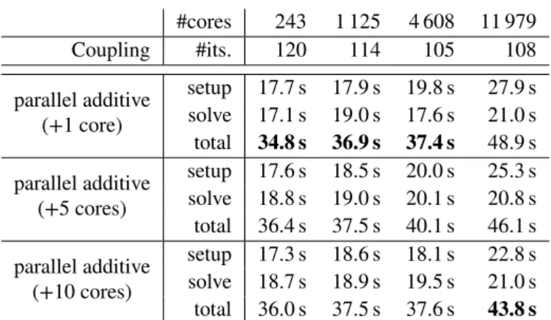
In section 5.3, we vary the number of cores used for the solution of the coarse problem in our best approach, i.e., the parallel additive coupling. As can be observed, increasing the number of cores from 1 to 10 yields a further speedup by more than 10 %.

We assume that a larger configuration with more cores will show an increasing advantage of the parallel additive approach.

However, a computation with 11 979 subdomains is the largest possible configuration of the backward facing step Stokes problem on our supercomputer.

#cores 243 1 125 4 608 11 979

Coupling #its. 120 114 105 108

parallel additive (+1 core)

setup 17.7 s 17.9 s 19.8 s 27.9 s solve 17.1 s 19.0 s 17.6 s 21.0 s total 34.8 s 36.9 s 37.4 s 48.9 s parallel additive

(+5 cores)

setup 17.6 s 18.5 s 20.0 s 25.3 s solve 18.8 s 19.0 s 20.1 s 20.8 s total 36.4 s 37.5 s 40.1 s 46.1 s parallel additive

(+10 cores)

setup 17.3 s 18.6 s 18.1 s 22.8 s solve 18.7 s 18.9 s 19.5 s 21.0 s total 36.0 s 37.5 s 37.6 s 43.8 s

TABLE 4Weak scalability results for monolithic preconditioners with SAS first level and parallel additive coupling applied to the three-dimensional BFS Stokes problem;H_h= 11, = 1h, and RGDSW Option 1. We allocate additional cores for the solution of the coarse problem (in brackets).

Recyling strategy #cores 243 1 125 4 608

-

#its. 155.25 (4) 158.3 (3) 149.0 (3)

setup 28.4 s 23.7 s 30.1 s

solve 40.5 s 37.7 s 42.2 s

total 68.9 s 61.4 s 72.3 s

SF

#its. 155.25 (4) 158.3 (3) 149.0 (3)

setup 24.1 s 20.3 s 25.6 s

solve 40.7 s 35.0 s 42.1 s

total 64.8 s 55.3 s 67.7 s

SF + CB

#its. 157.0 (4) 159 (3) 151.0 (3)

setup 18.7 s 16.7 s 21.8 s

solve 40.7 s 35.1 s 42.4 s

total 59.4 s 51.8 s 64.2 s

SF + CB + CM

#its. 165 (4) 175.3 (3) 170.3 (3)

setup 18.0 s 15.4 s 19.4 s

solve 42.8 s 38.0 s 46.3 s

total 60.8 s 53.4 s 65.7 s

TABLE 5Weak scalability results for monolithic preconditioners with coarse space recycling applied to the BFS Navier-Stokes problem;tolnl= 10^*6,H_h= 8, = 1h,⌫= 0.01,Re= 200, and RGDSW Option 1. SF, CB, and CM denote the reuse of the symbolic factorizations for the matricesA_iandA⁽ⁱ⁾_II, of the coarse basis , and of the coarse matrixA0, respectively. The times for the solution of a Stokes problem for the initial guess are included.

5.4 Recycling strategies

For nonlinear and time-dependent problems, we reuse information from the previous Newton or time iterations to save computing time. In particular, all index sets, e.g., corresponding to the overlapping subdomains and the interface components, are typically constant over all iterations and can safely be reused.

Whereas the entries of the system matrix change during Newton and time iterations, the nonzero pattern typically stays the same. Therefore, the symbolic factorizations of the local matrices and the global coarse matrix could be reused. Unfortunately, dropping small matrix entries in before the computation of the coarse RAP product (6) also saves compute time but changes the nonzero pattern of the coarse matrix. We observed that we save more time in the computation of the coarse RAP product by dropping small matrix entries in than by reusing the symbolic factorizations. We denote the reuse of the symbolic factorizations of the local overlapping matricesA_iand interior subdomain matricesA⁽ⁱ⁾_IIused in the saddle point extensions as theSF (Symbolic

FIGURE 6Solution of the time-dependent Navier-Stokes problem at time 1.0 s for the coronary artery; cf. section 2.2.

Factorization)recycling strategy. Note that, for a Navier-Stokes problem withH_h= 8and = 1h, the symbolic factorizations take between 15 and 20 % of the total factorization time for overlapping subdomain matrices A_i. The numeric factorization requires approximately 3.6 s, while the symbolic factorization requires 0.7 s. The effect is similar for interior subdomain matrices A⁽_IIⁱ⁾. For all following results we reuse the symbolic factorizations. Furthermore, we have observed that also reusing the numeric factorization of the matricesA_iis not a viable approach since it leads to significantly worse iteration counts.

With respect to the coarse level, we propose two recycling strategies, i.e., reusing the coarse basis but recomputing the coarse RAP product (6), denoted as theCB (Coarse Basis)recycling strategy, and reusing the coarse matrixA0and therefore saving time for computation of the coarse RAP product as well as for the coarse factorization, denoted as the CM (Coarse Matrix)recycling strategy.

A comparison of completely recomputing the preconditioner and three different combinations of the recycling strategies is presented in section 5.4 for a steady-state Navier-Stokes problem. As expected, the SF approach should always be preferred to completely recomputing the whole preconditioner. Furthermore, we observe that, for larger numbers of subdomains, the com- bination SF+CB is most efficient, whereas the scalability deteriorates for the combination SF+CB+CM. This can be explained by the fact that a recycled basis can still represent the null space of the operator, whereas a recycled coarse problem might be a bad approximation of the current linear tangent problem. In particular, we reach 69 % efficiency from 243 to 4 608 cores with basis recycling.

Further comparisons of the proposed recycling strategies for time-dependent problems are given in the next subsection. There, we observe a substantial increase in efficiency.

5.5 Speedup for a time-dependent Navier-Stokes problem

For small time steps, time-dependent problems are much better conditioned than their steady-state counterparts due to the added mass matrix. For certain problems, not even a coarse space is needed for numerical scalability; see, e.g.,⁵⁵, for the special case of a symmetric parabolic problem in two-dimensions. Nonetheless, for the time-dependent incompressible Navier-Stokes problem studied in this section, it is beneficial to use the RGDSW coarse space provided byFROSchsince the iteration counts are significantly lower; on average 82.8 iterations per timestep are required for the one level preconditioner, while only 38.5 iterations are required for the additive two-level method with coarse basis and coarse matrix recycling. Furthermore, by making use of the recycling methods presented in section 5.4, the additional time for the setup of the second level is neglectable. In section 5.5, we compare a one-level SAS preconditioner with two-level hybrid and additive SAS preconditioners. We compare coarse basis (SF+CB) and full recycling (SF+CB+CM) for the additive preconditioner and basis recycling for the hybrid preconditioner. We do not consider full recycling (SF+CB+CM) since we could not observe good convergence for the hybrid preconditioner with full recycling. This can be explained by the fact that the coarse operator has a larger effect if it is coupled in a multiplicative way. For the additive two-level preconditioner with full recycling, only 7.7 s are spend for the construction of second level once, namely in the first Newton iteration; 82.0 s of 480.5 s total computing time are spend on the application of the coarse level.

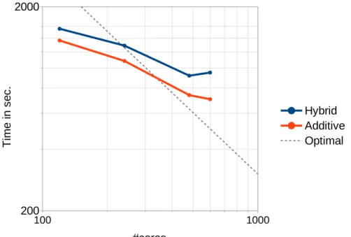
FIGURE 7Strong scaling results for time-dependent Navier-Stokes problem with 4.6 million d.o.f.. SAS for the first level with

= 1h. Hybrid two-level preconditioner with coarse basis recycling and additive two-level preconditioner with coarse basis and coarse matrix recycling. Simulation to final time of 1.0 s with t=0.01 s. Hier noch auf das Modellproblem verweisen.

FIGURE 8Timings for time-dependent Navier-Stokes problem with 4.6 million d.o.f. solved on 240 cores. SAS for the first level with = 1h. Hybrid and additive two-level preconditioners with different recycling strategies.

Recycling with a full reset, i.e., recomputing the coarse basis functions and the coarse matrix, after a certain number of time steps showed no advantage w.r.t total computing time.

In section 5.5, we present strong scaling results for the realistic artery. Here, we solve a problem with 4.6 million d.o.f. using a two-level additive RGDSW preconditioner with full recycling (SF+CB+CM) and a two-level hybrid RGDSW preconditioner with basis recycling (SF+CB). From 120 to 480 cores both preconditioners scale roughly equally well. However, the speedup for the hybrid preconditioner stagnates for more than 480 cores. This is not yet the case for the additive preconditioner. Therefore,

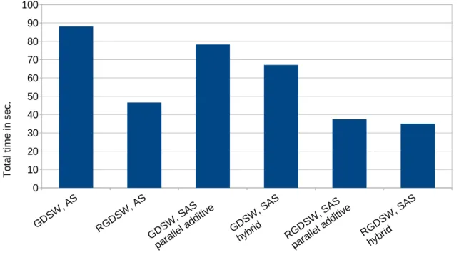
FIGURE 9Total time for the three-dimensional BFS Stokestol= 10^*6,H_h= 11, and = 1hon 4 608 cores. Improved pre- conditioner versions use SAS for the first level; cf. section 4.1. The improved (R)GDSW preconditioners with additive coupling between the levels use parallel coarse solves with 10 dedicated MPI ranks for the coarse problem; cf. section 4.4.

the additive preconditioner should be preferred for this configuration since the total computing time is between 5 % and 25 % faster than the hybrid preconditioner.

6 CONCLUSION

We have presented significant improvements to our monolithic GDSW preconditioner for incompressible fluid flow problems.

A combination of all presented strategies, i.e., using a reduced dimension coarse space, a scaled first level (SAS), and a multi- plicative coupling of the levels, reduces the time to solution by 60 % compared to the previous implementation for a BFS Stokes problem solved on 4 608 cores; cf. section 6 for timings.

For time-dependent and nonlinear problems, we can further make use of recycling of symbolic factorizations, the coarse basis, and the coarse matrix. Solving the 10 time steps of the coronary artery problem, we achieved a reduction of 75 % and 85 % for the best configurations with monolithic GDSW and RGDSW coarse spaces, respectively, compared to the previous implementation using the GDSW preconditioner; cf. section 6.

Our monolithic approach provides robustness and good parallel scalability for up to several thousand cores. Nonetheless, the preconditioner can be constructed in an algebraic fashion from the fully assembled saddle point system, and we are therefore able to provide a reduced and simple user interface to our implementation. Furthermore, unstructured meshes and domain decompositions are no restriction as they are handled in the same way as structured cases. The monolithic GDSW and RGDSW preconditioners are part of theFROSchframework in Trilinos and available to the public. Inexact local solvers for the first level as well as for the computation of saddle point harmonic extensions could reduce the setup time of our methods, and multi- level GDSW approaches could be considered to further improve the parallel scalability; cf.^56,57. Both are open topics for future research.

AcknowledgementsThe authors gratefully acknowledge financial support by the German Science Foundation (DFG), project no. KL2094/3- 2 and the computing time granted by the Center for Computational Sciences and Simulation (CCSS) of the University of Duisburg-Essen and provided on the supercomputer magnitUDE (DFG grants INST 20876/209-1 FUGG, INST 20876/243-1 FUGG) at the Zentrum für Informations- und Mediendienste (ZIM). We further thank the authors of⁴⁷for providing the realistic coronary artery geometry.

FIGURE 10Speedup for the time-dependent Navier-Stokes problem on 240 cores. Simulation of 0.1 s of the ramp phase, = 1h.

Improved preconditioner versions use SAS for the first level and full recycling; cf. section 4.1 and section 5.4, respectively.

References

1. Heinlein A, Hochmuth C, Klawonn A. Monolithic Overlapping Schwarz Domain Decomposition Methods with GDSW Coarse Spaces for Incompressible Fluid Flow Problems.Accepted for publication in SIAM J. Sci. Comput.2019.

2. Dohrmann CR, Klawonn A, Widlund OB. Domain decomposition for less regular subdomains: overlapping Schwarz in two dimensions.SIAM J. Numer. Anal.2008; 46(4): 2153–2168.

3. Dohrmann CR, Klawonn A, Widlund OB. A family of energy minimizing coarse spaces for overlapping Schwarz preconditioners. In: . 60 ofLect. Notes Comput. Sci. Eng.Berlin: Springer. 2008 (pp. 247–254).

4. Klawonn A, Pavarino L. Overlapping Schwarz methods for mixed linear elasticity and Stokes problems.Comput. Methods Appl. Mech. Engrg.1998; 165(1-4): 233–245.

5. Klawonn A, Pavarino L. A comparison of overlapping Schwarz methods and block preconditioners for saddle point problems.Numer. Linear Algebra Appl.2000; 7(1): 1–25.

6. Dohrmann CR. Some domain decomposition algorithms for mixed formulations of elasticity and incompressible fluids.in Workshop on Adaptive Finite Elements and Domain Decomposition Methods, Università degli Studi di Milano, Milan, Italy, 2010.

7. Benzi M, Golub GH, Liesen J. Numerical solution of saddle point problems.Acta Numer.2005; 14: 1–137.

8. Arrow KJ, Hurwicz L, Uzawa H, Chenery HB. Studies in linear and non-linear programming. 1958.

9. Bank RE, Welfert BD, Yserentant H. A class of iterative methods for solving saddle point problems.Numer. Math.1990;

56(7): 645–666.

10. Patankar S, Spalding D. A calculation procedure for heat, mass and momentum transfer in three dimensional parabolic flows.International J. on Heat and Mass Transfer1972; 15: 1787–1806.

11. Elman H, Silvester D. Fast nonsymmetric iterations and preconditioning for Navier-Stokes equations.SIAM J. Sci. Comput.

1996; 17(1): 33–46. Special issue on iterative methods in numerical linear algebra (Breckenridge, CO, 1994).

12. Klawonn A. Block-triangular preconditioners for saddle point problems with a penalty term.SIAM Journal on Scientific Computing1998; 19(1): 172–184.

13. Klawonn A. An optimal preconditioner for a class of saddle point problems with a penalty term.SIAM J. Sci. Comput.1998;

19(2): 540–552.

14. Klawonn A, Starke G. Block triangular preconditioners for nonsymmetric saddle point problems: field-of-values analysis.

Numer. Math.1999; 81(4): 577–594.

15. Rusten T, Winther R. A preconditioned iterative method for saddlepoint problems.SIAM J. Matrix Anal. Appl.1992; 13(3):

887–904.

16. Silvester D, Elman H, Kay D, Wathen A. Efficient preconditioning of the linearized Navier-Stokes equations for incom- pressible flow. In: Partial Differential Equations. Elsevier. 2001 (pp. 261-279).

17. Silvester D, Wathen A. Fast iterative solution of stabilised Stokes systems. II. Using general block preconditioners.SIAM J. Numer. Anal.1994; 31(5): 1352–1367.

18. Wathen A, Silvester D. Fast iterative solution of stabilised Stokes systems. I. Using simple diagonal preconditioners.SIAM J. Numer. Anal.1993; 30(3): 630–649.

19. Elman HC, Tuminaro RS. Boundary conditions in approximate commutator preconditioners for the Navier-Stokes equations.Electron. Trans. Numer. Anal.2009; 35: 257–280.

20. Kay D, Loghin D, Wathen A. A preconditioner for the steady-state Navier-Stokes equations.SIAM J. Sci. Comput.2002;

24(1): 237–256.

21. Silvester D, Elman H, Kay D, Wathen A. Efficient preconditioning of the linearized Navier-Stokes equations for incom- pressible flow.J. Comput. Appl. Math.2001; 128(1-2): 261–279.

22. Elman H, Howle VE, Shadid J, Shuttleworth R, Tuminaro R. Block preconditioners based on approximate commutators.

SIAM J. Sci. Comput.2006; 27(5): 1651–1668 (electronic).

23. Quarteroni A, Saleri F, Veneziani A. Analysis of the Yosida method for the incompressible Navier-Stokes equations.J.

Math. Pures Appl. (9)1999; 78(5): 473–503.

24. Quarteroni A, Saleri F, Veneziani A. Factorization methods for the numerical approximation of Navier-Stokes equations.

Comput. Methods Appl. Mech. Engrg.2000; 188(1-3): 505–526.

25. Benzi M, Ng M, Niu Q, Wang Z. A relaxed dimensional factorization preconditioner for the incompressible Navier-Stokes equations.J. Comput. Phys.2011; 230(16): 6185–6202.

26. Benzi M, Guo XP. A dimensional split preconditioner for Stokes and linearized Navier-Stokes equations.Appl. Numer.

Math.2011; 61(1): 66–76.

27. Deparis S, Grandperrin G, Quarteroni A. Parallel preconditioners for the unsteady Navier-Stokes equations and applications to hemodynamics simulations.Comput. & Fluids2014; 92: 253–273.

28. Bramble JH, Pasciak JE. A domain decomposition technique for Stokes problems.Appl. Numer. Math.1990; 6(4): 251–261.

29. Tuminaro RS, Tong CH, Shadid JN, Devine KD, Day D. On a multilevel preconditioning module for unstructured mesh Krylov solvers: two-level Schwarz.Communications in Numerical Methods in Engineering; 18(6): 383-389.

30. Cai XC, Keyes DE, Marcinkowski L. Non-linear additive Schwarz preconditioners and application in computational fluid dynamics.Internat. J. Numer. Methods Fluids2002; 40(12): 1463–1470.