Technical Report Series
Center for Data and Simulation Science
Alexander Heinlein, Mauro Perego, Sivasankaran Rajamanickam
FROSch Preconditioners for Land Ice Simulations of Greenland and Antarctica
Technical Report ID: CDS-2021-01
Available at https://kups.ub.uni-koeln.de/id/eprint/30668
Submitted on January 25, 2021
GREENLAND AND ANTARCTICA
2
ALEXANDER HEINLEIN
†, MAURO PEREGO
‡, AND SIVASANKARAN RAJAMANICKAM
‡3
Abstract. Numerical simulations of Greenland and Antarctic ice sheets involve the solution of 4
large-scale highly nonlinear systems of equations on complex shallow geometries. This work is con- 5
cerned with the construction of Schwarz preconditioners for the solution of the associated tangent 6
problems, which are challenging for solvers mainly because of the strong anisotropy of the meshes and 7
wildly changing boundary conditions that can lead to poorly constrained problems on large portions 8
of the domain. Here, two-level GDSW (Generalized Dryja–Smith–Widlund) type Schwarz precondi- 9
tioners are applied to di↵erent land ice problems, i.e., a velocity problem, a temperature problem, 10
as well as the coupling of the former two problems. We employ the MPI-parallel implementation 11
of multi-level Schwarz preconditioners provided by the package FROSch (Fast and Robust Schwarz) 12
from the Trilinos library. The strength of the proposed preconditioner is that it yields out-of-the-box 13
scalable and robust preconditioners for the single physics problems.
14
To our knowledge, this is the first time two-level Schwarz preconditioners are applied to the 15
ice sheet problem and a scalable preconditioner has been used for the coupled problem. The pre- 16
conditioner for the coupled problem di↵ers from previous monolithic GDSW preconditioners in the 17
sense that decoupled extension operators are used to compute the values in the interior of the sub- 18
domains. Several approaches for improving the performance, such as reuse strategies and shared 19
memory OpenMP parallelization, are explored as well.
20
In our numerical study we target both uniform meshes of varying resolution for the Antarctic ice 21
sheet as well as non uniform meshes for the Greenland ice sheet are considered. We present several 22
weak and strong scaling studies confirming the robustness of the approach and the parallel scalability 23
of the FROSch implementation. Among the highlights of the numerical results are a weak scaling 24
study for up to 32 K processor cores (8 K MPI-ranks and 4 OpenMP threads) and 566 M degrees of 25
freedom for the velocity problem as well as a strong scaling study for up to 4 K processor cores (and 26
MPI-ranks) and 68 M degrees of freedom for the coupled problem.
27
Key words. domain decomposition methods, monolithic Schwarz preconditioners, GDSW 28
coarse spaces, multiphysics simulations, parallel computing 29
AMS subject classifications. 65F08, 65Y05, 65M55, 65N55 30
1. Introduction. Greenland and Antarctic ice sheets store most of the fresh
31
water on earth and mass loss from these ice sheets significantly contributes to sea-
32
level rise (see, e.g. [11]). In this work, we propose overlapping Schwarz domain
33
decomposition preconditioners for efficiently solving the linear systems arising in the
34
context of ice sheet modeling.
35
We first consider the solution of the ice sheet momentum equations for com-
36
puting the ice velocity. This problem is at the core of ice sheet modeling and
37
has been largely addressed in literature and several solvers have been considered
38
[40, 6, 18, 35, 50, 19, 10, 9]. Most solvers from the literature rely on Newton-
39
Krylov methods, using, e.g., the conjugate gradient (CG) [31] or the generalized
40
minimal residual (GMRES) [44] method as the linear solver, and either one-level
41
⇤
Submitted to the editors DATE.
†
Institute for Applied Analysis and Numerical Simulation, University of Stuttgart, Germany.
Department of Mathematics and Computer Science, University of Cologne (alexander.heinlein@uni- koeln.de). Center for Data and Simulation Science, University of Cologne (http://www.cds.uni-koeln.
de).
‡
Center for Computing Research, Scalable Algorithms Department, Sandia National Laboratories
(mperego@sandia.gov, srajama@sandia.gov). Sandia National Laboratories is a multimission labo-
ratory managed and operated by National Technology and Engineering Solutions of Sandia, LLC.,
a wholly owned subsidiary of Honeywell International, Inc., for the U.S. Department of Energy’s
National Nuclear Security Administration under contract DE-NA-0003525.
Schwarz preconditioners, hierarchical low-rank methods, or multigrid preconditioners
42
to accelerate the convergence. In particular, the ones that have been demonstrated
43
on problems with hundreds of millions of unknowns [6, 35, 50, 19, 10] use tailored
44
multigrid preconditioners or hierarchical low-rank methods. Multigrid precondition-
45
ers [6, 35, 50, 19] require careful design of the grid transfer operators for properly
46
handling the anisotropy of the mesh and the basal boundary conditions that range
47
from no-slip to free-slip. Hierarchical low-rank approaches have also been used for the
48
velocity problem [10, 9]. Chen et al. [10] developed a parallel hiearchical low-rank
49
preconditioner that is aysmptotically scalable, but it has a large constant overhead
50
and the trade-o↵ between memory usage and solver convergence does not make it
51
an ideal choice for the large problems considered here. The hierarchical low-rank
52
approach that showed the most promise in terms of solver scalability is a sequential
53
implementation limiting its usage to small problems [9].
54
In addition to the velocity problem, we also consider the problem of finding the
55
temperature of an ice sheet using an enthalpy formulation ([1, 46, 32]) and the steady-
56
state thermo-mechanical problem coupling the velocity and the temperature problems.
57
The robust solution of this coupled problem is crucial for finding the initial thermo-
58
mechanical state of the ice sheet under the assumption that the problem is almost
59
at thermodynamic equilibrium. In fact, the initial state is estimated solving a PDE-
60
constrained optimization problem where the loss function is the mismatch with ob-
61
servations and the constraint is the coupled velocity-temperature problem considered
62
here. To our knowledge, while there are works in the literature targeting the solution
63
of unsteady versions of the coupled problem ([5, 39, 43]), none of them targets the
64
steady thermo-mechanical problem at the ice sheet scale.
65
Both the velocity problem and the coupled velocity-temperature problem are
66
characterized by strong nonlinearities and anisotropic meshes (due to the shallow
67
nature of ice sheets). The coupled problem presents additional complexities due to the
68
di↵erent nature of the velocity and temperature equations, the former being a purely
69
di↵usive elliptic problem, whereas the second is an advection dominated problem. In
70
our experience, the naive use of multigrid methods leads to convergence failure for
71
the coupled problem.
72
Our approach is to employ a preconditioning framework based on two-level Schwarz
73
methods with GDSW (Generalized Dryja–Smith–Wildund) [12, 13, 22, 23] type coarse
74
spaces. To our knowledge, scalable domain decomposition methods such as the GDSW
75
preconditioner used in this work have not been shown to work on the ice sheet prob-
76
lems. The main contributions of this work are:
77
• We demonstrate that two-level Schwarz preconditioners such as GDSW (Gen-
78
eralized Dryja–Smith–Widlund) type preconditioners work out-of-the-box to
79
solve two single physics problems (the velocity problem and the temperature
80
problem) on land ice simulations.
81
• We introduce a scalable two-level preconditioner for the coupled problem that
82
is tailored for the coupled problem by decoupling the extension operators to
83
compute the values in the interior of the subdomains.
84
• We present results using an MPI-parallel implementation of multi-level Schwarz
85
preconditioners provided by the package FROSch (Fast and Robust Schwarz)
86
from the Trilinos software framework.
87
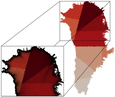
• Finally, we demonstrate the scalability of the approach with several weak
88
and strong scaling studies confirming the robustness of the approach and
89
the parallel scalability of the FROSch implementation. We conduct a weak
90
scaling study for up to 32 K processor cores and 566 M degrees of freedom for
91
the velocity problem as well as a strong scaling study for up to 4 K processor
92
cores and 68 M degrees of freedom for the coupled problem. We compare
93
against the multigrid method in [48, 50] for the velocity problem.
94
The remainder of the paper is organized as follows. Sections 2 and 3 introduces the ice
95
sheet problems and the finite element discretization used in this study. We describe
96
the Schwarz precondtioners, the reuse strategies for better performance and the way
97
we tailor the preconditioner for the coupled problem in Section 4. Our software
98
framework, which is based on Albany and FROSch, is briefly described in Section
99
5. Finally, the scalability and the performance of the proposed preconditioners are
100
shown in Section 6.
101
2. Mathematical model. At the scale of glaciers and ice sheets, ice can be
102
modeled as a very viscous shear-thinning fluid with a rheology that depends on the
103
ice temperature. Complex phenomena like the formation of crevasses and ice calving
104
would require more complex damage mechanics models, however the fluid descrip-
105
tion accounts for most of the large scale dynamics of ice sheets and it is adopted
106
by all ice sheet computational models. The ice temperature depends on ice flow
107
(velocity/deformation). Given the large characteristic time scale of the temperature
108
evolution, it is reasonable to assume the temperature to be relatively constant over
109
a few decades and solve the flow problem uncoupled from the temperature problem.
110
However, when finding the initial state of an ice sheet (by solving an inverse problem)
111
it is important to consider the coupled flow/temperature model, to find a self con-
112
sistent initial thermo-mechanical state. In this case, we assume the ice temperature
113
to be almost in steady-state. Therefore, in this paper, we consider a steady-state
114
temperature solver. In this section, we first introduce separately the flow model and
115
the temperature model and then the coupled model.
116
2.1. Flow model. We model the ice as a very viscous shear-thinning fluid with velocity u and pressure p satisfying the Stokes equations:
⇢ r · (u, p) = ⇢ i g, r · u = 0,
where g is the gravity acceleration, ⇢ i the ice density and the stress tensor. In what
117
follows, we use the so called first-order (FO) or Blatter-Pattyn approximation of the
118
Stokes equations derived using scaling arguments based on the fact that ice sheets are
119
shallow. Following [42] and [47], we have
120
⇢ r · (2µ ✏ ˙ 1 ) = ⇢ i g @ x s, r · (2µ ✏ ˙ 2 ) = ⇢ i g @ y s, (2.1)
121
where x and y are the horizontal coordinate vectors in a Cartesian reference frame,
122
s(x, y) is the ice surface elevation, g = | g | , and ˙ ✏ 1 and ˙ ✏ 2 are given by
123
(2.2) ✏ ˙ 1 = 2 ˙ ✏ xx + ˙ ✏ yy , ✏ ˙ xy , ✏ ˙ xz
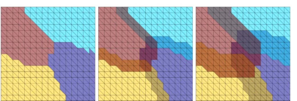
T and ✏ ˙ 2 = ✏ ˙ xy , ✏ ˙ xx + 2 ˙ ✏ yy , ✏ ˙ yz . T .
124
Denoting with u and v the horizontal components of the velocity u, the stress com-
125
ponents are defined as ✏ xx = @ x u, ✏ xy = 1 2 (@ y u + @ x v), ✏ yy = @ y v, ✏ xz = 1 2 @ z u and
126
✏ yz = 1 2 @ z v. The ice viscosity µ in Eq. (2.1) is given by
127
(2.3) µ = 1
2 A(T )
n1✏ ˙
1 n
e
n,
128
where A(T ) = ↵ 1 e ↵
2T is a temperature-dependent rate factor (see [47] for the defi-
129
nition of coefficients ↵ 1 and ↵ 2 ), n = 3 is the power-law exponent, and the e↵ective
130
strain rate, ˙ ✏, is defined as
131
(2.4) ✏ ˙ e ⌘ ✏ ˙ 2 xx + ˙ ✏ 2 yy + ˙ ✏ xx ✏ ˙ yy + ˙ ✏ 2 xy + ˙ ✏ 2 xz + ˙ ✏ 2 yz
1 2
,
132
where ˙ ✏ ij are the corresponding strain-rate components. Given that the atmospheric
133
pressure is negligible compared to the pressure in the ice, we prescribe stress-free
134
conditions at the the upper surface:
135
(2.5) ✏ ˙ 1 · n = ˙ ✏ 2 · n = 0,
136
where n is the outward pointing normal vector at the ice sheet upper surface, z =
137
s(x, y). The lower surface can slide according to the following Robin-type boundary
138
condition
139
2µ e ✏ ˙ 1 · n + u = 0, 2µ˙ ✏ 2 · n + v = 0,
140
where is a spatially variable friction coefficient and u and v are the horizontal
141
components of the velocity u. The field is set to zero beneath floating ice. On
142
lateral boundaries we prescribe the conditions
143
(2.6) 2µ˙ ✏ 1 · n = 1
2 gH ⇢ i ⇢ w r 2 n 1 and 2µ ✏ ˙ 2 · n = 1
2 gH ⇢ i ⇢ w r 2 n 2 ,
144
where n is the outward pointing normal vector to the lateral (i.e., parallel to the (x, y)
145
plane), ⇢ w is the density of ocean water, n 1 and n 2 are the x and y component of n,
146
and r is the ratio of ice thickness that is submerged. On terrestrial ice margins r = 0,
147
whereas on floating ice r = ⇢ ⇢
wi. Additional details on the momentum balance solver
148
can be found in [47].
149
2.2. Temperature model. As apparent from (2.3), the ice rheology depends on the ice temperature T . In order to model the ice sheet thermal state, we consider an enthalpy formulation similar to the one proposed by Aschwanded et al. in [1]. We assume that, for cold ice, the enthalpy h depends linearly on the temperature, whereas for temperate ice, the enthalpy grows linearly with the water content
h =
⇢ ⇢ i c (T T 0 ), for cold ice (h h m ), h m + ⇢ w L , for temperate ice.
Here, the melting enthalpy h m is defined as h m := ⇢ w c(T m T 0 ) and T 0 is a uniform
150
reference temperature.
151
The steady state enthalpy equation reads
152
(2.7) r · q(h) + u · r h = 4µ ✏ 2 e .
153
Here, q(h) is the enthalpy flux, given by
q(h) = ( k
⇢
ic
ir h, for cold ice (h h m ),
k
⇢
ic
ir h m + ⇢ w Lj(h), for temperate ice,
u · r h is the drift term, and 4µ ✏ 2 e is the heat associated to ice deformation. The water flux term
j(h) := 1
⌘ w
(⇢ w ⇢ i )k 0 g
has been introduced by Schoof and Hewitt ([46, 32]), and it describes the percolation of water driven by gravity. The parameter c i is the heat capacity of ice, k its thermal conductivity, and L is the latent heat of fusion. At the upper surface, the enthalpy is set to h = ⇢ i c(T s T 0 ), where T s is the temperature of the air at the ice upper surface.
At the bed, the ice is either in contact with a dry bed or with a film of water at the melting point temperature and, in first approximation, satisfies the Stefan condition:
m = G + p
u 2 + v 2 k r T · n and m (T T m ) = 0 and T m 0.
Here, m is the melting rate. Ice at the bed is melting when m > 0 and refreezing
154
when m < 0. Moreover, G is the geothermal heat flux (positive if entering the ice
155
domain), p
u 2 + v 2 is the frictional heat, and k r T · n is the temperature heat flux
156
exiting the domain as n is the outer normal to the ice domain. Depending on whether
157
the ice is cold at the bed, melting or refreezing, the Stefan condition translates into
158
natural or essential boundary conditions for the enthalpy equation. Further details
159
on the enthalpy formulation and its discretization are provided in [41].
160
2.3. Coupled model. The ice velocity depends on the temperature through
161
(2.4), and the enthalpy depends on the velocity field through the drift term u · r h
162
and the fractional heat term at the ice sheet lower surface. The first order problem
163
(2.1) only provides the horizontal velocities u and v, but we also need the vertical
164
velocity w to solve the enthalpy equations. The vertical velocity w is computed using
165
the incompressibility condition
166
(2.8) @ x u + @ y v + @ z w = 0,
167
with the Dirichlet boundary condition at the ice lower surface u · n = m
L (⇢ i ⇢ w ) .
The coupled problem is formed by problems (2.1), (2.8) and (2.7) and their respective
168
boundary conditions. For further details, see [41]. Figure 1 shows the ice velocity and
169
temperature computed solving the coupled thermo-mechanical model. For details
170
about the problem setting and the Greenland data set, see [41].
171
3. Finite element discretization. The ice sheet mesh is generated by extrud-
172
ing in the vertical direction a two dimensional unstructured mesh of the ice sheet
173
horizontal extension ([47]) and it is constituted of layers of prisms. The problems
174
described in section 2 are discretized with continuous piece-wise bi-linear (for trian-
175
gular prisms) or tri-linear (for hexahedra) finite elements using a standard Galerkin
176
formulation, for each component of the velocity and for the enthalpy. We use up-
177
wind stabilization for the enthalpy equation. The nonlinear discrete problems can be
178
written in the residual form
179
F (x) = 0, (3.1)
180 181
where x is the problem unknown (velocity, enthalpy, or both, depending on the prob-
182
lem). The nonlinear problems are then solved using a Newton-Krylov approach. More
183
precisely, we linearize the problem using Newton’s method, and solve the resulting
184
linear tangent problems
185
DF (x (k) ) x (k) = F (x (k) ) (3.2)
186 187
Fig. 1. Solution of a Greenland ice sheet simulation. Left: ice surface speed in [m/yr], Right:
ice temperature in [K] over a vertical section of the ice sheet.
using a Krylov subspace method. The Jacobian DF is computed through automatic
188
di↵erentiation. At each nonlinear iteration, we solve a problem of the form
189
Ax = r, (3.3)
190 191
where A is the tangent matrix DF (x (k) ), and r is the residual vector F (x (k) ). Using
192
a block matrix notation, the tangent problem of the velocity problem can be written
193
as
194
A uu A uv
A vu A vv
x u
x v =
r u
r v
(3.4)
195 196
where the tangent matrix is symmetric positive definite. When considering also the
197
vertical velocity w, the tangent problem becomes
198
2
4 A uu A uv
A vu A vv
A wu A wu A ww
3 5
| {z }
=:A
u2 4 x u
x v
x w
3 5
| {z }
=:x
u= 2 4 r u
r v
r w
3 5
| {z }
=:r
u(3.5)
199
200
Note that the matrix is lower block-triangular because in the FO approximation, the
201
horizontal velocities are independent of the vertical velocity. Similarly, the tempera-
202
ture equation reads
203
A T x T = r T . (3.6)
204 205
The coupled problem is a multiphysics problem coupling the velocity and the
206
temperature problem. Hence, the tangent system can be written as
207
A u C uT
C T u A T
x u
x T =
˜ r u
˜ r T , (3.7)
208
209
Fig. 2. Extending two-dimensional nonoverlapping subdomains (left) by layers of elements to obtain overlapping domain decompositions with an overlap of = 1h (middle) and = 2h (right).
where the blocks A u and A T and solution vectors x u x T are the same as in the single
210
physics problems; cf. (3.5) and (3.6). The residual vectors ˜ r u and ˜ r T di↵er from the
211
single physics residuals r u and r T due to the coupling of velocity and temperature,
212
which also results in the nonzero coupling blocks coupling blocks C uT and C T u in the
213
tangent matrix.
214
4. Preconditioners. In order to solve the tangent problems (3.2) in our Newton
215
iteration, we apply the generalized minimal residual (GMRES) method [44] and speed
216
up the convergence using generalized Dryja–Smith–Widlund (GDSW) type domain
217
decomposition preconditioners. In particular, we will use classical GDSW and reduced
218
dimension GDSW (RGDSW) preconditioners, as described in subsection 4.1, as well
219
as corresponding monolithic preconditioners, as introduced in subsection 4.3. In order
220
to improve the performance of the first level of the Schwarz preconditioners, we will
221
always apply scaled prolongation operators; cf. subsection 4.2. As we will describe
222
in subsection 4.4, domain decomposition preconditioners and, in particular, GDSW
223
type preconditioners are well-suited for the solution of land ice problems because
224
of the specific structure of the meshes. In order to improve the efficiency of the
225
preconditioners in our Newton-Krylov algorithm, we will also apply strategies to reuse,
226
in later Newton iterations, certain components of the preconditioners set up in the
227
first Newton iteration; see subsection 4.5.
228
For the sake of clarity, we will restrict ourselves to the case of uniform meshes
229
with characteristic element size h for the description of the preconditioners. However,
230
the methods can also be applied to non-uniform meshes as the ones for Greenland;
231
see Figure 4.
232
4.1. GDSW type preconditioners. Let us consider the general linear system
233
Ax = b (4.1)
234 235
arising from a finite element discretization of an elliptic boundary value problem on
236
⌦. Our aim is then to apply the preconditioners to the tangent problems (3.3) of the
237
model problems described in section 2.
238
The GDSW preconditioner was originally introduced by Dohrmann, Klawonn,
239
and Widlund in [13, 12] for elliptic problems. It is a two-level Schwarz preconditioner
240
with energy minimizing coarse space and exact solvers. To describe the construction
241
of the GDSW preconditioner, let ⌦ be partitioned into N nonoverlapping subdomains
242
⌦ 1 , ..., ⌦ N with characteristic size H . We extend these subdomains by adding k layers
243
of finite elements resulting in overlapping subdomains ⌦ 0 1 , ..., ⌦ 0 N with an overlap
244
= kh; cf. Figure 2 for a two-dimensional example. In general, two-level Schwarz
245
preconditioners for (4.1) with exact solvers are of the form
246
M OS 2 = A 0 1 T
| {z }
coarse level
+ X N i=1
R i T A i 1 R i
| {z }
first level
. (4.2)
247
248
Here, A 0 = T A is the coarse matrix corresponding to a Galerkin projection onto
249
the coarse space, which is spanned by the columns of matrix . The local matrices A i 250
are submatrices of A corresponding to the overlapping subdomains ⌦ 0 1 , ..., ⌦ 0 N . They
251
can be written as A i = R i AR T i , where R i : V h ! V i h is the restriction operator from
252
the global finite element space V h to the local finite element space V i h on ⌦ 0 i ; the R T i
253
is the corresponding prolongation.
254
We first present the framework enabling the construction of energy-minimizing
255
coarse spaces for elliptic problems based on a partition of unity on the interface
256
= x 2 (⌦ i \ ⌦ j ) \ @⌦ D | i 6 = j, 1 i, j N (4.3)
257 258
of the nonoverlapping domain decomposition, where @⌦ D is the Dirichlet boundary.
259
This will allow us to construct classical GDSW coarse spaces [13, 12] and reduced
260
dimension GDSW coarse spaces [16] as used in our simulations. Note that other
261
types of coarse spaces can be constructed using this framework as well, e.g., coarse
262
spaces based on the MsFEM (Multiscale Finite Element Method) [34]; see also [7].
263
However, in our experiments, we restrict ourselves to the use of GDSW type coarse
264
spaces.
265
Let us first decompose into connected components 1 , ..., M . This decom-
266
position of may be overlapping or nonoverlapping. Furthermore, let R
ibe the
267
restriction from all interface degrees of freedom to the degrees of freedom of the in-
268
terface component i . In order to account for overlapping decompositions of the
269
interface, we introduce diagonal scaling matrices D
i, such that
270
X M i=1
R T
iD
iR
i= I , (4.4)
271 272
where I is the identity matrix on . This means that the scaling matrices correspond
273
to a partition of unity on the interface .
274
Using the scaling matrices D
i, we can now build a space which can represent the
275
restriction of the null space of our problem to the interface. Therefore, let the columns
276
of the matrix Z form a basis of the null space of the operator ˆ A, which is the global
277
matrix corresponding to A but with homogeneous Neumann boundary conditions on
278
the full boundary, and let the Z be restriction of Z to the interface . Because of
279
(4.4), we have
280
X M i=1
R T
iD
iR
iZ = Z .
281 282
Now, for each i , we construct a matrix
isuch that its columns are a basis of
283
the space spanned by the columns of D
iR
iZ . Then, the interface values of our
284
coarse space are given by the matrix
285
(4.5) = ⇥
R T
1 1... R T
M M⇤ .
286
Based on these interface values, the coarse basis functions are finally computed
287
as energy-minimizing extensions to the interior of the nonoverlapping subdomains.
288
Therefore, we partition all degrees of freedom into interface ( ) and interior (I) degrees
289
of freedom. Then, the system matrix can written as
290
A =
A II A I
A I A
291 292
and the energy-minimizing extensions are computed as I = A II 1 A I , resulting
293
in the coarse basis
294
(4.6) =
I =
A II 1 A I
.
295
As mentioned earlier, this construction allows for a whole family of coarse spaces,
296
depending on decomposition of the interface into components i and the choice of
297
scaling matrices D
i.
298
GDSW coarse spaces. We obtain the interface components of the GDSW coarse
299
space (GDSW) i by decomposing the interface into the largest connected components
300
belonging to the same sets of subdomains N , i.e., into vertices, edges, and faces;
301
cf., e.g., [38]. More precisely,
302
N := i : x 2 ⌦ i 8 x 2 .
303
Because these components are disjoint by construction, the scaling matrices D
(GDSW)i
304
have to be chosen as identity matrices I
(GDSW)i
in order to satisfy (4.4). Using this
305
choice, we obtain the classical GDSW coarse space as introduced by Dohrmann, Kla-
306
wonn, and Widlund in [13, 12]. If the boundaries of the subdomains are uniformly
307
Lipschitz, the condition number estimate for the resulting two-level GDSW precondi-
308
tioner,
309
M GDSW 1 A C
✓
1 + H ◆ ✓ 1 + log
✓ H h
◆◆
, (4.7)
310 311
holds for scalar elliptic and compressible linear elasticity model problems; the constant
312
C is then independent of the geometrical parameters H, h, and . For the general case
313
of ⌦ ⇢ R 2 being decomposed into John domains, we can obtain a condition number
314
estimate with a second power logarithmic term, i.e., with 1 + log H h 2 instead of
315
1 + log H h ; cf. [12, 13]. Please also refer to [14, 15] for other variants with linear
316
logarithmic term.
317
RGDSW coarse spaces. Another choice of the i leads to reduced dimension
318
GDSW (RGDSW) coarse spaces; cf. [16]. In order to construct the interface com-
319
ponents (RGDSW) i , we first define a hierarchy of the previously defined (GDSW) i . In
320
particular, we call an interface component ancestor of another interface compo-
321
nent 0 if N
0⇢ N ; conversely, we call o↵spring of 0 if N
0N . Now, let
322
ˆ (GDSW)
i i=1,...,M
(RGDSW)be the set of all GDSW interface components which have
323
no ancestors; we call these coarse components. Now, we define the RGDSW interface
324
components as
325
(RGDSW)
i := [
N ⇢N
ˆ(GDSW)i
, 8 i = 1, ..., M (RGDSW) . (4.8)
326
327
The (RGDSW) i may overlap in nodes which do not belong to the coarse components.
328
Hence, we have to introduce scaling operators D
(RGDSW)i
6 = I
(RGDSW)i
to obtain a
329
partition of unity on the interface; cf. (4.4). Di↵erent scaling operators D
ilead to
330
di↵erent variants of RGDSW coarse spaces, e.g., Options 1, 2.1, and 2.2, introduced
331
in [16] and another variant introduced in [25]. Here, we will only consider the algebraic
332
variant, Option 1, where an inverse multiplicity scaling
333
D
(RGDSW)i
= R
(RGDSW)i
![Fig. 1. Solution of a Greenland ice sheet simulation. Left: ice surface speed in [m/yr], Right:](https://thumb-eu.123doks.com/thumbv2/1library_info/3752721.1510349/7.918.123.648.143.458/solution-greenland-sheet-simulation-left-surface-speed-right.webp)