Technical Report Series Center for Data and Simulation Science

Technical Report Series

Center for Data and Simulation Science

Matthias Eichinger, Alexander Heinlein, Axel Klawonn

Stationary flow predictions using convolutional neural networks

Technical Report ID: CDS-2019-20

Available at https://kups.ub.uni-koeln.de/id/eprint/10440

Submitted on December 16, 2019

Stationary flow predictions using convolutional neural networks

Matthias Eichinger

, Alexander Heinlein

, and Axel Klawonn

1 Introduction

Computational Fluid Dynamics (CFD) simulations are a numerical tool to model and analyze the behavior of fluid flow. They are used in a wide range of application areas, such as, e.g., civil and mechanical engineering, meteorology or medical science, a wide range of different fluids and settings. In CFD simulations, the input parameters are classically the material parameters of the fluid, such as density and viscosity, the geometry of the computational domain, and the boundary conditions as well as volume forces. Transient simulations, additionally depend on the initial condition.

Depending on the underlying model for the fluid flow, the resulting flow field may depend on all these input parameters in a highly nonlinear way. Furthermore, CFD simulations often require a high spatial and temporal resolution in order to obtain accurate results. Therefore, CFD simulations are generally very compute intensive.

The complexity of CFD simulations may be reduced using, e.g., Proper Orthog- onal Decomposition (POD), Reduced Basis (RB), or simplified physics methods;

these techniques are all Model Order Reduction (MOR) techniques. In this work, we propose a different approach, which can also be regarded as a MOR technique. In particular, we propose to use appropriate neural networks as surrogate models for CFD simulations; cf. Figure 1. As for MOR techniques, we will have to perform many CFD simulations in advance in a very expensive offline phase. However, the evaluation of the trained model will then be much faster compared to a CFD simu- lation. Here, we focus on predicting the fluid flow with respect to variations in the geometry of the computational domain. Therefore, we consider a steady flow prob- lem in order to eliminate the time-dependence of the flow field and the dependence

1 Department of Mathematics and Computer Science, University of Cologne, Weyertal 86- 90, 50931 Köln, Germany. E-mail:{alexander.heinlein,axel.klawonn}@uni-koeln.de, eichingm@smail.uni-koeln.de.

2Center for Data and Simulation Science, University of Cologne, Germany, url: http://www.cds.uni- koeln.de

1

2 Matthias Eichinger, Alexander Heinlein, and Axel Klawonn

Geometry Material parameters

Initial conditions

Boundary conditions &

Volume forces

CFD simulations Classical approach

Neural network Surrogate model

Flow field

Fig. 1 Our approach is to train a neural network as a surrogate model for CFD simulations. Here, we do not consider varying initial conditions, material parameters, boundary conditions, or volume forces but focus on varying geometries for the computational domain.

of the solution on an initial condition. Furthermore, we keep the material parameters, as well as boundary conditions and volume forces constant.

A different approach for the prediction of fluid flow using neural networks for fixed geometries can be found in, e.g., [9, 10].

Our approach is inspired by the work of Guo, Li, and Iorio [6], where the authors used a Convolutional Neural Network (CNN) to predict the steady flow around obstacles in a channel. In our work, we further extend this approach by using the more complex network architecture of the U-Net, which was introduced in [11], and considering different types of loss functions. In particular, we will compute synthetic training data from CFD simulations using OpenFOAM 5.0 [5] and train CNNs using Keras 2.2.4 [2] with Tensorflow 1.12 [1] backend to approximate the resulting flow fields.

This paper is organized as follows: in section 2, we describe our model problem and the computation of the reference data using CFD simulations. Next, we describe the CNN architectures and the training settings used for our surrogate model in section 3. Section 4 shows the performance of our models on training and validation data as well as the generalization properties for some types of unseen data. Finally, we present a short conclusion and outlook.

2 CFD simulations

Let us consider computational domains

:=

6] × [0, 3] \

6] ×

3] is a polygonal star-shaped domain; see Figure 2.

The stationary flow of an incompressible Newtonian fluid with kinematic viscosity

0 within the computational domain

is modeled by the steady Navier-Stokes equations,

−ν∆u+(u· ∇)u+∇p= f

in

∇ ·u=

0 in

(1)

∂Ωin

∂Ω_wall

∂Ωout

∂Ωwall

∂Ωwall

δΩwallType I

Type II

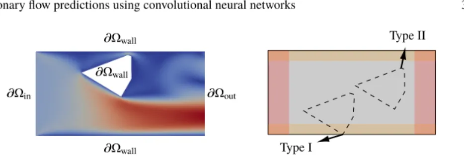
Fig. 2 Left: the computational domain is a channel of length 6 and width 3 with a polygonal obstacle. Right: type I obstacles are connected with the bottom wall, type II obstacles have a distance of 0.75 to each part of the boundary (yellow). Both types of obstacles have a distance of 1.5 to the inlet and the outlet (red) and may not cover more than 50 % of the cross section of the channel.

with velocity

and pressure

:= 0

3] and

:= 6

3] be the inlet and outlet, respectively, and

:=

0, 6

0

0, 6

3

be the remainder of the boundary of

. We prescribe

u=

3 on

∂u

∂n −pn=

0 on

and

0 on

as boundary conditions; cf. Figure 2 for an exemplary resulting flow field. Here,

is the outward pointing normal vector.

In order to perform the CFD simulations, we employ the CFD software Open- FOAM 5.0 [5], which is based on the FVM (Finite Volume Method). In particular, we first use SnappyHexMesh to generate compute meshes from STL (Standard Tri- angle Language) files that describe the polygonal obstacles. Secondly, we compute corresponding stationary flow fields using the SimpleFoam solver.

Since we fix all parameters and boundary conditions, the resulting flow field only depends on the shape and location of the polygonal obstacle

we only consider two different types of obstacles here: obstacles that are connected with the bottom wall and obstacles that are not connected with any part of the boundary of the channel.

3 Surrogate Convolutional Neural Network

To predict fluid flow using neural networks, we fix the structure of the input and output

data of our models. Whereas, in numerical CFD simulations, the structure and size

of the compute mesh and the solution vector may differ significantly for different

configurations, neural network rely on structured data. Therefore, our approach is to

4 Matthias Eichinger, Alexander Heinlein, and Axel Klawonn

Input data Output data

Binary

SDF

0 1

<0

>0

ux

uy

Fig. 3 Generation of structured input data (left) and output data (right) for training the neural networks. As input, we generate a 256×128 pixel image with a binary or SDF representation of the obstacle. As output, we interpolate the componentsuxanduyof the flow field on a 256×128 pixel image.

convert both the input, i.e., the description of the obstacle geometry, and the output, i.e., the flow field, to 256

128 pixel images; cf. Figure 3. As input, we either use a binary representation of the geometry, i.e., 0 if the center of a pixel is covered by the obstacle and 1 otherwise, or a Signed Distance Function (SDF) representation, i.e., the value in each pixel is the smallest distance of its center to the boundary of the obstacle multiplied with

1 if the center lies within the obstacle. As output, we interpolate the

and

components of the flow field to 256

128 pixel images.

Due to their good performance on image data, we apply CNNs in order to ap- proximate the nonlinear relation between out input and output data. In particular, we consider the CNN used in [6] as well as the U-Net [11] with both one and two de- coder paths and Rectified Linear Unit (ReLU) activation; for more details on neural network, see, e.g., [4, 12].

Furthermore, we consider a total of 100 000 data sets (50 000 type I and 50 000 type II obstacles) consisting of an equally many polygons with 3, 4, 5, 6, and 12 edges, respectively; the shapes and sizes of the polygons are randomly chosen under the conditions described in Figure 2. Out of the 100 000 data sets, we randomly select 90 000 as training data and 10 000 as validation data. We optimize applying a Stochastic Gradient Descent (SGD) method with a batch size of 64 and an adaptive scaling of the learning rate using the Adam (Adaptive moments) [8] algorithm with an initial learning rate

0.001. We use a maximum of 300 epochs for the training and reduce the learning rate by 20 % in case of stagnation for more than 50 epochs.

In case of SDF input data, we apply Z-normalization, and in case of binary input data, we use batch normalization [7]. Our implementation uses Keras 2.2.4 [2] with Tensorflow 1.12 [1] backend.

Even though, our neural networks may be very complex with approximately 50 million parameters on average, their evaluation is still much cheaper compared to corresponding CFD simulations; on a single core of an AMD Threadripper 2950X (8

×

3.8 Ghz), the evaluation of our neural network models (less than 0.01 s) was more

than two orders of magnitude faster than the average CFD simulation (approximately

50 s). On GPU (Graphics Processing Unit) architectures, the speedup will be even

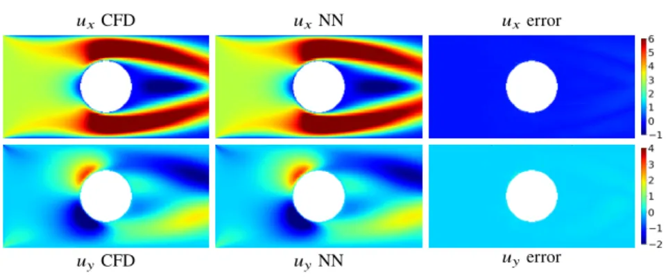
ux CFD uxNN uxerror

uyCFD uyNN uyerror

Fig. 4 Comparison of the ground truth flow field (left) computed in a CFD simulation, the prediction by a neural network (middle), and the pointwise error (right) for an example with low averaged relative error (2) is 2 %.

u_x CFD u_xNN u_xerror

u_yCFD u_yNN uyerror

Fig. 5 Comparison of the ground truth flow field (left) computed in a CFD simulation, the prediction by a neural network (middle), and the pointwise error (right) for an example with higher averaged relative error (2) is 31 %.

larger. However, the training of the neural networks, which includes the computation of the training data using CFD simulations, may take hours or even days.

We refer to [3] for a detailed discussion of the employed models, our software framework, as well as a more detailed discussion the different types of obstacles and a discussion of techniques for efficient generalization to other types of obstacles.

In [3], we will also discuss the speedup of our neural networks compared to the CFD

simulations in more detail.

6 Matthias Eichinger, Alexander Heinlein, and Axel Klawonn

CNN [6] U-Net [11]

Input # Dec. Loss Total Type I Type II Total Type I Type II

SDF 1

MSE 61.16 % 110.46 % 11.86 % 17.04 % 29.42 % 4.66 % MSE+(2) 3.97 % 3.31 % 4.63 % 2.67 % 2.11 % 3.23 % MAE 25.19 % 41.52 % 8.86 % 9.10 % 13.89 % 4.32 % MAE+(2) 4.45 % 3.84 % 5.05 % 2.48 % 1.87 %3.10 % 2

MSE 49.82 % 89.12 % 10.51 % 13.01 % 21.59 % 4.42 % MSE+(2) 3.85 % 3.05 % 4.64 % 2.43 % 1.78 % 3.23 % MAE 45.23 % 81.38 % 9.08 % 5.47 % 7.06 % 3.89 % MAE+(2) 4.33 % 3.74 % 4.91 % 2.57 % 1.98 % 3.17 %

Binary 1

MSE 49.78 % 88.28 % 11.28 % 27.15 % 49.15 % 5.15 % MSE+(2) 10.12 % 11.44 % 8.80 % 5.49 % 6.25 % 4.74 % MAE 39.16 % 64.77 % 13.54 % 15.69 % 26.36 % 5.02 % MAE+RE 10.61 % 12.34 % 8.87 % 4.48 % 5.05 % 3.90 % 2

MSE 51.34 % 91.20 % 11.48 % 24.00 % 43.14 % 4.85 % MSE+(2) 10.03 % 11.37 % 8.69 % 5.56 % 6.79 % 4.33 % MAE 37.16 % 62.01 % 12.32 % 21.54 % 38.12 % 4.96 % MAE+(2) 9.53 % 10.91 % 8.15 % 6.04 % 7.88 % 4.20 % Table 1 Comparison of the performance of different CNN models based on the error (2). The best error rates for a given CNN architecture and input type are marked inbold face.

4 Results

In order to measure the performance of our neural networks, we first introduce our error measure. Therefore, let

be the set of all polygons

in the set of validation data and

be the set of all non-obstacle pixels for one specific polygonal obstacle

averaged relative error

1

|V| Õ

P∈V

1

|I_P| Õ

p∈IP

ku_p−u

ˆ

ku_pk₂+

10

(2)

with

and ˆ

being the reference velocity, computed in a CFD simulation, and the predicted velocity, computed by evaluating the neural networks, respectively. The term 10

acts as a regularization in case of very low reference velocities

.

We compare the CNN from [6] to the U-Net [11] using one and two decoder paths using binary and SDF input data. Furthermore, we will observe that the performance depends significantly on the loss function used to train the neural network. As the loss function, we compare four different choices, i.e., the Mean Squared Error (MSE), the sum of the MSE and the averaged relative error (2), the Mean Absolute Error (MAE), and the sum of the MAE and the averaged relative error (2).

Performance on the original data

As can be seen in Figures 4 and 5, the predic-

tion may be very good but may also show qualitative and quantitative differences to

the reference solution. However, if a good combination of the network architecture,

the type of input data, the number of decoder paths, and the loss function is used,

ux CFD uxNN uxerror

uyCFD uyNN uyerror

Fig. 6 Generalization properties for the U-Net with one decoder path, MAE+(2) loss function, and SDF input data: comparison the ground truth flow field (left) computed in a CFD simulation, the prediction by the neural network (middle), and the pointwise error (right). Circular obstacles were not part of the training data of the CNN. The averaged relative error (2) is 3 %.

SDF Input Binary Input

Polygon # Edges Total Type I Type II Total Type I Type II 7 2.71 % 1.89 % 3.53 % 4.39 % 4.61 % 4.16 % 8 2.82 % 1.98 % 3.65 % 4.67 % 4.89 % 4.44 % 10 3.21 % 2.32 % 4.10 % 5.23 % 5.51 % 4.94 % 15 4.01 % 3.16 % 4.86 % 7.76 % 7.85 % 6.66 % 20 5.08 % 4.22 % 5.93 % 9.70 % 10.43 % 8.97 %

Table 2 Generalization properties of the U-Net with one decoder path, and MAE+(2) loss function.

Error (2) for polygon types which were not in the data set used for training: 1 000 polygons (500 type I and 500 type II) for each different number of edges.

the average performance of the CNN model over all data is very convincing; see Table 1. Compared to the worst configuration with a total averaged error of 61.16 %, the optimal configuration, using the U-Net [11], SDF input, two decoder paths, and MSE+(2) loss function, the total averaged error can be reduced to 2.43 %. Using only one decoder path and MAE+(2) loss function yields comparable results but results in a reduction of the number of parameters of the CNN by more than 30 %.

The choice of the network architecture and the loss function have the greatest influence on the performance of the model. In particular, the U-Net generally per- forms much better than the other CNN, and a combination of MSE or MAE with (2) improves then performance significantly compared to only using MSE or MAE.

Generalization properties

In order to investigate the generalization properties,

we now only consider the U-Net architecture with one decoder path, and MAE+(2)

loss function and only vary the type of input data. This model performed very well

for the training and validation data but is more efficient compared to the models

with two decoder paths. In Figure 6, we present the flow field for a circular obstacle,

which was not part of the training and validation data. It can be observed that the

averaged relative error (2) for this example is only 3 %. The very good generalization

8 Matthias Eichinger, Alexander Heinlein, and Axel Klawonn

properties of our model are also apparent in the results in Table 2, which shows the results for several different types of polygonal obstacles which were not part of the training and validation data. The maximum total averaged error is below 10 %.

These results confirm that the neural network is able to generalize to other types of polygonal obstacles and is not overfitted to training data.

5 Conclusion

In this work, we have shown that CNNs may serve as efficient surrogate models for CFD simulations. We have focussed on the dependence of the flow field on the geometry of the computational domain, and the extension of this framework to, e.g., varying boundary conditions or material parameters will be future work.

Due to the limited available space, we are not able to discuss, e.g, further gen- eralization techniques for our models or to compare computing times of the CFD simulations and the CNNs in detail. We refer to [3] for a more detailed discussion.

References

1. M. Abadi, A. Agarwal, P. Barham, E. Brevdo, Z. Chen, C. Citro, G. S. Corrado, A. Davis, J. Dean, M. Devin, S. Ghemawat, I. Goodfellow, A. Harp, G. Irving, M. Isard, Y. Jia, R. Joze- fowicz, L. Kaiser, M. Kudlur, J. Levenberg, D. Mané, R. Monga, S. Moore, D. Murray, C. Olah, M. Schuster, J. Shlens, B. Steiner, I. Sutskever, K. Talwar, P. Tucker, V. Vanhoucke, V. Va- sudevan, F. Viégas, O. Vinyals, P. Warden, M. Wattenberg, M. Wicke, Y. Yu, and X. Zheng.

TensorFlow: Large-scale machine learning on heterogeneous systems, 2015. Software available from tensorflow.org.

2. F. Chollet et al. Keras. https://keras.io, 2015.

3. M. Eichinger, A. Heinlein, and A. Klawonn. Flow predictions using convolutional neural networks. In preparation, 2019.

4. I. Goodfellow, Y. Bengio, and A. Courville.Deep learning, volume 1. MIT press Cambridge, 2016.

5. C. J. Greenshields. Openfoam user guide, v5. 0.OpenFOAM foundation Ltd, 2017.

6. X. Guo, W. Li, and F. Iorio. Convolutional neural networks for steady flow approximation. In Proceedings of the 22Nd ACM SIGKDD International Conference on Knowledge Discovery and Data Mining, KDD ’16, pages 481–490, New York, NY, USA, 2016. ACM.

7. S. Ioffe and C. Szegedy. Batch normalization: Accelerating deep network training by reducing internal covariate shift.arXiv:1502.03167, 2015.

8. D. P. Kingma and J. Ba. Adam: A method for stochastic optimization.1412.6980, 2014.

9. M. Raissi, P. Perdikaris, and G. E. Karniadakis. Physics informed deep learning (part i):

Data-driven solutions of nonlinear partial differential equations.arXiv:1711.10561, 2017.

10. M. Raissi, P. Perdikaris, and G. E. Karniadakis. Physics informed deep learning (part ii):

Data-driven discovery of nonlinear partial differential equations.arXiv:1711.10566, 2017.

11. O. Ronneberger, P. Fischer, and T. Brox. U-net: Convolutional networks for biomedical image segmentation. Medical Image Computing and Computer-Assisted Intervention – MICCAI 2015, pages 234–241, 2015.

12. J. Watt, R. Borhani, and A. K. Katsaggelos. Machine Learning Refined: Foundations, Algo- rithms, and Applications. Cambridge University Press, 2016.