Technical Report Series
Center for Data and Simulation Science
Alexander Heinlein, Martin Lanser
Additive and Hybrid Nonlinear Two-Level Schwarz Methods and Energy Minimizing Coarse Spaces for Unstructured Grids
Technical Report ID: CDS-2019-17
Available at https://kups.ub.uni-koeln.de/id/eprint/9845
Submitted on July 23, 2019
METHODS AND ENERGY MINIMIZING COARSE SPACES FOR UNSTRUCTURED GRIDS⇤
ALEXANDER HEINLEIN† ‡ AND MARTIN LANSER† ‡
Abstract. Nonlinear domain decomposition (DD) methods, such as, e.g., ASPIN (Additive Schwarz Preconditioned Inexact Newton), RASPEN (Restricted Additive Schwarz Preconditioned Inexact Newton), Nonlinear-FETI-DP, or Nonlinear-BDDC methods, can be reasonable alternatives to classical Newton-Krylov-DD methods for the solution of sparse nonlinear systems of equations, e.g., arising from a discretization of a nonlinear partial di↵erential equation. These nonlinear DD approaches are often able to e↵ectively tackle unevenly distributed nonlinearities and outperform Newton’s method with respect to convergence speed as well as global convergence behavior. Fur- thermore, they often improve parallel scalability due to a superior ratio of local to global work.
Nonetheless, as for linear DD methods, it is often necessary to incorporate an appropriate coarse space in a second level to obtain numerical scalability for increasing numbers of subdomains. In addition to that, an appropriate coarse space can also improve the nonlinear convergence of nonlinear DD methods.
In this paper, four variants how to integrate coarse spaces in nonlinear Schwarz methods in an additive or multiplicative way using Galerkin projections are introduced. These new variants can be interpreted as natural nonlinear equivalents to well-known linear additive and hybrid two- level Schwarz preconditioners. Furthermore, they facilitate the use of various coarse spaces, e.g., coarse spaces based on energy-minimizing extensions, which can easily be used for irregular domain decompositions, as, e.g., obtained by graph partitioners. In particular, Multiscale Finite Element Method (MsFEM) type coarse spaces are considered, and it is shown that they outperform classical approaches for certain heterogeneous nonlinear problems.
The new approaches are then compared with classical Newton-Krylov-DD and nonlinear one- level Schwarz approaches for di↵erent homogeneous and heterogeneous model problems based on the p-Laplace operator.
Key words. Nonlinear preconditioning, inexact Newton methods, nonlinear Schwarz methods, nonlinear domain decomposition, multiscale coarse spaces, ASPIN, RASPEN
AMS subject classifications. 65F08, 65F10, 65H10, 65H20, 65N12, 65N22, 65N30, 65N55
1. Introduction. We are concerned with the e↵ective solution of nonlinear sys- tems of equations using nonlinear domain decomposition (DD) methods. These non- linear systems arise, e.g., by finite element discretization of the variational formulation of a nonlinear partial di↵erential equation. Let therefore V be a finite element space discretizing a computational domain⌦⇢Rd, d= 2,3,and
(1) F(u) = 0,
a certain nonlinear system of equations given by the nonlinear functionF :V !V, with the solutionu2V. In this paper, for the sake of clarity, we will restrict ourselves to the two-dimensional case, however our approaches can be easily extended to three dimensions as well.
Besides classical Newton-Krylov-DD methods, where the nonlinear system(1)is linearized with Newton’s method and the tangential system is solved with a conjugate
⇤Preliminary ideas on one of four new nonlinear two-level Schwarz methods together with first Matlab experiments have been already presented in a proceedings paper; see [30]. The present paper significantly extends those preliminary ideas and also contains other new algorithms and numerical results.
†Department of Mathematics and Computer Science, University of Cologne, Weyertal 86-90, 50931 K¨oln, Germany,{alexander.heinlein, martin.lanser}@uni-koeln.de, url: http://www.numerik.
uni-koeln.de
‡Center for Data and Simulation Science, University of Cologne,http://www.cds.uni-koeln.de 1
gradient (CG) or generalized minimal residual method (GMRES) approach precondi- tioned by some DD preconditioner, in recent years, nonlinear domain decomposition methods became popular. These approaches often yield faster convergence, especially if the initial value is outside the area of quadratic convergence of Newton’s method.
In nonlinear DD methods, the computational domain⌦is decomposed into nonover- lapping or overlapping subdomains. A corresponding decomposition of the nonlinear problem is then used to construct nonlinear left- or right-preconditioners. In contrast, to linear DD preconditioners or methods, which improve only the convergence of the linear solvers, nonlinear DD preconditioners can also positively a↵ect the nonlinear convergence.
Nonlinear right-preconditioners are often associated with a nonlinear elimination procedure, as, e.g., described in [9]. Many di↵erent variants have been developed in the last two decades leading to di↵erent nonlinear DD methods, such as nonlinear FETI (Finite Element Tearing and Interconnecting) [46,47,31], Nonlinear-FETI-DP (Finite Element Tearing and Interconnecting - Dual Primal) [41,39,38,37], Nonlin- ear BDDC (Balancing Domain Decomposition by Constraints) [37,40], or nonlinear elimination preconditioned inexact Newton [33, 35]. In these approaches, the sets of variables which are eliminated in a nonlinear fashion are either chosen based on a nonoverlapping domain decomposition [46, 47, 31, 41, 39, 38, 37, 40] or problem dependent using a heuristic approach, e.g., based on the nonlinear residual [33,35].
In this paper, we consider nonlinear left-preconditioners based on a nonoverlap- ping domain decomposition, i.e., nonlinear Schwarz preconditioners. While nonlinear Schwarz methods as iterative approaches have already been developed and analyzed in [4,17,44,50], a nonlinear Schwarz preconditioner was first suggested in [5] and the resulting method was called ASPIN (Additive Schwarz Preconditioned Inexact New- ton). In [5], also the corresponding exact approach was derived, which can be denoted by ASPEN (Additive Schwarz Preconditioned Exact Newton). Both approaches of- ten yield superior nonlinear convergence compared to classical Newton-Krylov-DD approaches. This is also investigated numerically in [2], where ASPIN is compared with various combinations of nonlinear solvers designed for a fast nonlinear conver- gence. Both, ASPIN and ASPEN, were introduced as one-level methods and the numerical scalability of the preconditioned linear systems for an increasing number of subdomains is therefore generally not ensured. Thus, several approaches to implement a second level have been proposed: an additive nonlinear coarse problem based on a coarser mesh [6,45], an additive linear coarse problem [34], and a multiplicative vari- ant using an FAS (full approximation scheme) update [15]. In the latter publication, also a restricted variant of ASPEN, called RASPEN (Restricted Additive Schwarz Preconditioned Exact Newton), is introduced; restricted Schwarz methods typically improve the linear convergence compared to standard overlapping Schwarz methods.
In this paper, we introduce four di↵erent additively and multiplicatively coupled two-level (R)ASPEN and (R)ASPIN methods based on Galerkin projections instead of an FAS update. The multiplicative coupling between coarse space and local cor- rections is comparable to the MSPIN approach [43]. One of our four approaches was already discussed in [30]. The inexact tangential systems of our methods are nat- urally equivalent to linear systems preconditioned with the well-known additive or hybrid Schwarz preconditioners described in, e.g., [51]; therefore, the methods can be interpreted as the natural nonlinear equivalents to classical linear two-level Schwarz methods. We combine these methods with coarse spaces designed for irregular domain decompositions as provided by graph partitioners, as, e.g., METIS [36], and numer- ically prove a superior nonlinear as well as linear convergence behavior compared to
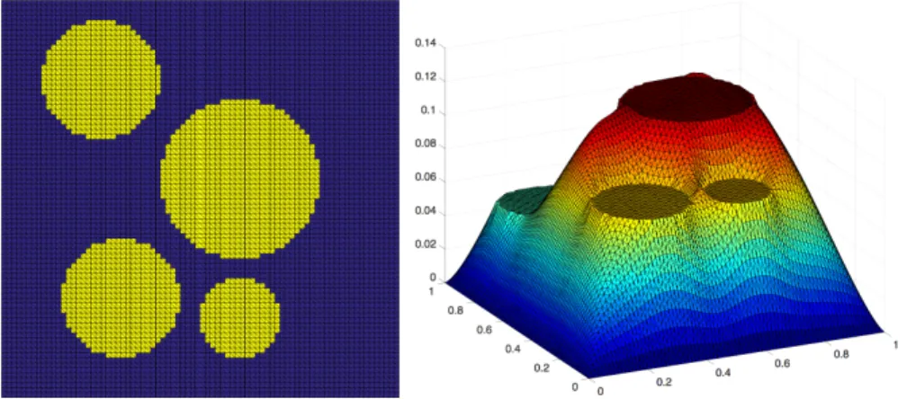
Fig. 1.Left: Circular inclusions; coefficient distribution with↵= 103or↵= 106in the yellow part and↵ = 1in the remaining blue part. Right: Solution of the corresponding heterogeneous model problem with a high coefficient of↵= 106.
one-level (R)ASPIN or (R)ASPEN methods and the corresponding Newton-Krylov- Schwarz approaches. Let us remark that these coarse spaces can theoretically also be used with FAS-RASPEN, but in this case, the coarse basis functions have to be pro- vided in the dual space; seesubsection 5.2for more details. This is not necessary in our approaches. Despite of this, our nonlinear two-level algorithms and FAS-RASPEN share similar building blocks, which have similar computational costs.
2. Model problems. Our model problems are based on the scaled p-Laplace operator, which is defined by
↵ pu:= div(↵|ru|p 2ru)
forp 2. We then consider the model problem: findu2H01(⌦), such that
(2) ↵ pu = 1 in ⌦
u = 0 on@⌦, where↵:⌦!Ris a coefficient function.
Here, we always consider the casep= 4 and two di↵erent coefficient distributions:
first, ahomogeneous model problem, i.e.,↵(x) = 1 for all x2⌦, and second, a heterogeneous model problemwith a high coefficient in four circles and↵(x) = 1 in the remaining area; seeFigure 1(left) for the coefficient distribution andFigure 1 (right) for the corresponding solution. We present numerical results insection 8.
3. Nonlinear one-level Schwarz methods. Let us first describe the one-level nonlinear Schwarz method introduced in [5], which is also the basis for our new meth- ods. The inexact variant is well-known under the name ASPIN and a restricted reformulation named RASPEN was first introduced in [15]. In both approaches, the nonlinear problem(1)is reformulated into an equivalent nonlinear problemF(u) = 0 before Newton’s method is applied. The reformulation is obtained from the solution of many local nonlinear problems on parts of⌦and can be interpreted as a nonlinearly left-preconditioned functionF(u) =G(F(u)). Here,Gis only known implicitly.
We define a decomposition of⌦into nonoverlapping subdomains⌦i, i= 1, ..., N, where each subdomain is the union of finite elements. By adding k layers of finite
elements to the subdomains, overlapping subdomains⌦0i, i = 1, ..., N with overlap
=khare constructed, where h is the diameter of a finite element. We denote by Vi the local finite element spaces associated to the overlapping subdomains⌦0i. With restrictionsRi:V !Viand prolongationsPi:Vi!V, we can define local nonlinear correctionsTi(u) as the solutions of the local problems
(3) RiF(u PiTi(u)) = 0, i= 1, ..., N.
In [5], it is shown that the nonlinear equation
(4) FA(u) :=FASPEN(u) :=
XN
i=1
PiTi(u) = 0
has the same solution as (1). Solving (4) using Newton’s method, i.e., with the iteration
u(k+1)=u(k) ⇣
DFA(u(k))⌘ 1 FA⇣
u(k)⌘ , yields the ASPEN approach. The derivative ofFA(u) writes (5) DFA(u) =
XN
i=1
PiDTi(u) = XN
i=1
Pi(RiDF(ui)Pi) 1RiDF(ui),
withui=u PiTi(u) andDTi(u) obtained by deriving(3). Replacingui byuin(5) yields the inexact tangent of the ASPIN approach. Consequently, the tangent of the ASPIN approach is equal toMOS1DF(u), where MOS1 is the linear one-level additive Schwarz preconditioner applied for the tangentDF(u).
Let us note that for both evaluations,DFA(u(k)) andFA(u(k)), the local nonlin- ear problems defined in(3)have to be solved in each Newton iteration. This is usually done by an inner Newton iteration carried out independently on each overlapping sub- domain. In the remainder of this paper, we call Newton iterations on the subdomains inner iterationsand denote global Newton iterations by the outer iteration. For an algorithmic description of ASPIN or ASPEN, see, e.g., [5, 15] orsection 7.
Alternatively, one can also use the restricted Schwarz approach described in [7]
to construct a nonlinear preconditioner; cf. [15]. We therefore define restricted pro- longation operatorsPei:Vi!V, i= 1, ..., N, such that
XN
i=1
PeiRi=I
is fulfilled; this means that the prolongation operators form a partition of unity on⌦.
With the equation
(6) FRA(u): =FRASPEN(u) :=
XN
i=1
PeiTi(u)= 0,
linearization with Newton’s method leads to the RASPEN method u(k+1)=u(k) ⇣
DFRA(u(k))⌘ 1
FRA⇣ u(k)⌘
,
with the derivative (7) DFRA(u) =
XN
i=1
PeiDTi(u) = XN
i=1
Pei(RiDF(ui)Pi) 1RiDF(ui).
Therefore, ASPEN and RASPEN only di↵er by the prolongation from the subdomains to the complete domain and thus by the combination of the nonlinear correction terms Ti(u); the local correction terms themselves will be identical if they are computed for the same functionu. Moreover, the inexact tangent of the nonlinear RASPIN method is equivalent to the restricted two-level Schwarz preconditioned linear system.
4. Nonlinear two-level Schwarz methods. In this section, we describe our approach to add a nonlinear coarse level to ASPEN or RASPEN. Our approach di↵ers from the two-level variants described in [15,34,6,45] and we will discuss the di↵er- ences later, in section 5. In this section, we assume that a restrictionR0 :V !V0
to a given coarse spaceV0 and a corresponding prolongationP0 :V0 !V are given.
Throughout this article, we always use P0 := RT0. Coarse spaces for linear Schwarz methods are typically given by a finite element discretization on an additional coarse triangulation or by constructing coarse basis functions exploiting the domain decom- position. Insection 6, we will discuss the construction of coarse spaces for nonlinear Schwarz methods and unstructured domain decompositions without the need for an additional coarse triangulation.
Based onR0 and P0, let us define the nonlinear coarse correction T0(u) as the solution of the nonlinear equation
(8) R0F(u P0T0(u)) = 0
for a given u 2 V. Therefore, we exclusively consider nonlinear coarse functions F0 :V0 !V0 which can be defined by a Galerkin approach asF0(u0) :=R0F(P0u0) for any u0 2V0. In this paper, we will consider four di↵erent approaches to add a coarse level to the ASPEN or RASPEN method:
• in an additive fashion,
• in a multiplicative fashion before the nonlinear subdomain corrections are applied,
• in a multiplicative fashion after the nonlinear subdomain corrections are applied,
• or in a multiplicative fashion before and after the nonlinear subdomain corrections are applied.
Let us remark that we already discussed the third variant in [30] and presented some preliminary numerical results. All four variants lead to di↵erent nonlinear problems and therefore also di↵erent linearized systems. Consequently, both, the nonlinear and the linear convergence behavior, may di↵er; cf.section 8. We will now give a detailed description of the four approaches based on the ASPEN framework.
4.1. Additive coupling. We first define the additive nonlinear two-level oper- ator
(9) Fadd(u) :=Fadditive(u) :=
XN
i=1
PiTi(u) +P0T0(u).
A linearization ofFadd(u) = 0 using Newton’s method leads to an additive two-level ASPEN method
u(k+1)=u(k) ⇣
DFadd(u(k))⌘ 1
Fadd⇣ u(k)⌘
,
with the derivative
(10)
DFadd(u) = PN i=1
PiDTi(u) +P0DT0(u)
= PN i=1
Pi(RiDF(ui)Pi) 1RiDF(ui) +P0(R0DF(u0)P0) 1R0DF(u0),
whereui=u PiTi(u), i= 0, ..., N, as before. The derivativeDT0(u) is obtained by deriving(8).
In accordance to linear Schwarz operators, as defined, e.g., in [51], we introduce nonlinear Schwarz operators
(11) Qi(u) :=Pi(RiDF(u)Pi) 1RiDF(u), such that(10)can be rewritten as
(12) DFadd(u) =
XN
i=0
Qi(ui).
We refer to this method as A-ASPEN, where “A” indicates the additive coupling of the levels.
4.2. Multiplicative coupling – coarse problem first. The second nonlinear two-level operator is defined by
(13) Fh,1(u) :=Fhybrid,1(u) :=
XN
i=1
PiTi(u P0T0(u)) +P0T0(u).
Applying Newton’s method to the corresponding nonlinear equation Fh,1(u) = 0 yields a hybrid two-level ASPEN method
u(k+1)=u(k) ⇣
DFh,1(u(k))⌘ 1
Fh,1⇣ u(k)⌘
, with the derivative
(14)
DFh,1(u) = PN i=1
PiDTi(u P0T0(u)) (I P0DT0(u)) +P0DT0(u)
= I
✓ I
PN i=1
Qi(vi)
◆
(I Q0(u0)).
Here, we haveu0=u P0T0(u),vi=u0 PiTi(u0), andQi as defined in(11).
We refer to this method as H1-ASPEN, where “H1” indicates a multiplicative coupling where the coarse operator is applied before the local corrections.
4.3. Multiplicative coupling – coarse problem second. We define another nonlinear two-level operator with multiplicative coupling, where the coarse problem is solved after the local corrections have been applied. It is defined by
(15) Fh,2(u) :=Fhybrid,2(u) :=
XN
i=1
PiTi(u) +P0T0(u XN
i=1
PiTi(u)).
The corresponding Newton iteration for solvingFh,2(u) = 0 is given by u(k+1)=u(k) ⇣
DFh,2(u(k))⌘ 1
Fh,2⇣ u(k)⌘
, with the derivative
(16)
DFh,2(u) = PN i=1
PiDTi(u) +P0DT0
⇣u PN
i=1PiTi(u)⌘ ⇣
I PN
i=1PiDTi(u)⌘
= I (I Q0(v0))
✓ I
PN i=1
Qi(ui)
◆ , where ui =u PiTi(u) andv0 =u PN
i=1PiTi(u) P0T0(u PN
i=1PiTi(u)), and Qi as defined in(11).
We refer to this method as H2-ASPEN, where “H2” indicates a multiplicative coupling where the coarse operator is applied after the local corrections.
4.4. Multiplicative coupling – symmetric variant. In order to simplify the notation, we first define v := u P0T0(u) and w := v
PN i=1
PiTi(v). Then, the symmetric nonlinear two-level operator is then defined by
(17) Fh(u) =Fhybrid(u) :=P0T0(w) + XN
i=1
PiTi(v) +P0T0(u).
We obtain the Newton iteration of the symmetric hybrid two-level ASPEN method u(k+1)=u(k) ⇣
DFh(u(k))⌘ 1
Fh⇣ u(k)⌘
for the solution ofFh(u) = 0. The derivatives ofv andwwith respect touare given by
Dv=I P0DT0(u) =I Q0(u0) and
Dw= I P0DT0(u) PN i=1
PiDTi(v) (I P0DT0(u))
=
✓ I
PN i=1
Qi(vi)
◆
(I Q0(u0)),
withu0=u P0T0(u), andvi=v PiTi(v), i= 1, ..., N. With this in mind, we can derive the jacobian
(18)
DFh(u) = P0DT0(w)Dw+PN
i=1
PiDTi(v)Dv+P0DT0(u)
= I (I Q0(w0))
✓ I PN
i=1
Qi(vi)
◆
(I Q0(u0)).
Here, we have againu0 =u P0T0(u) and vi = v PiTi(v), i = 1, ..., N as well as w0=w P0T0(w);Qi is defined in(11).
We refer to this method as H-ASPEN, where “H” indicates a multiplicative cou- pling where the coarse operator is applied twice, i.e., before and after the local cor- rections. Let us finally remark that the computational cost for each Newton step of H-RASPEN is slightly higher, since the nonlinear coarse problem has to be solved twice.
4.5. Inexact and restricted variants. All four approaches can be extended to corresponding inexact or restricted variants in a straight-forward way.
In particular, when using u as the linearization point for all nonlinear Schwarz operators, we obtain ASPIN variants of our nonlinear two-level Schwarz methods
DFadd(u)⇡ XN
i=0
Qi(u),
DFh,1(u)⇡I I XN
i=1
Qi(u)
!
(I Q0(u)),
DFh,2(u)⇡I (I Q0(u)) I XN
i=1
Qi(u)
! , and
DFh(u)⇡I (I Q0(u)) I XN
i=1
Qi(u)
!
(I Q0(u)).
In particular, these variants are equivalent to applying the corresponding additive or hybrid linear two-level Schwarz preconditioners to the tangentDF(u).
Furthermore, using the restricted prolongation operators Pei instead of Pi, i = 1, ..., N, to add the local corrections in the nonlinear Schwarz preconditioners leads directly to the corresponding RASPEN or RASPIN variants; cf.section 3.
5. Di↵erences to existing two-level methods. In the literature, two di↵erent existing nonlinear two-level Schwarz preconditioners can be found. First, an additive variant is described in [45,6] and second, a multiplicative approach is chosen in [15].
Additionally, in [34], a linear second level is introduced, which we do not consider here.
5.1. Additive nonlinear coarse space. In this subsection, we describe the additive approach to implement a nonlinear coarse problem chosen in [45, 6] and discuss the similarities and di↵erences to our approach. First, we assume that we have a nonlinear coarse problem
(19) F0(u⇤0) = 0
with the unique solution u⇤0 and F0 : V0 ! V0. The nonlinear function F0 can be obtained by a Galerkin approach as before or, e.g., by a coarser finite element discretization of the nonlinear partial di↵erential equation.
Finally, in [45,6], the coarse correctionC0(u) is implicitly defined by the equation
(20) F0(C0(u)) =R0F(u)
and the nonlinear operator by
(21) FCKM(u) :=P0C0(u) P0C0(u⇤) + XN
i=1
PiTi(u).
Here, u⇤ is the solution of the original nonlinear problem (1). Let us note that with(20)we haveC0(u⇤) =u⇤0, which can be obtained by solving(19). A linearization using Newton’s method leads to
u(k+1)=u(k) ⇣
DFCKM(u(k))⌘ 1
FCKM⇣ u(k)⌘
,
with the derivative (22)
DFCKM(u) = PN i=1
PiDTi(u) +P0DC0(u)
=PN
i=1
Pi(RiDF(ui)Pi) 1RiDF(ui) +P0(DF0(C0(u))) 1R0DF(u).
The derivativeDC0(u) is thereby obtained by a derivation of (20)and we haveui = u PiTi(u), i= 0, ..., N, as before.
In contrast to our approaches, also coarse functions F0 which are not obtained by a Galerkin approach can be used. Therefore, this approach is more general in that sense. Especially considering a coarse problem arising from a discretization on a coarse triangulation can save compute time, since the assembly of the problem is less costly. Nonetheless, we intend to use nonlinear coarse problems which can also be used for unstructured meshes and domain decompositions; seesection 6. Therefore, we construct coarse spaces based on a Galerkin approach. A disadvantage of the approach from [45, 6] is that (19) has to be solved in advance to compute C0(u⇤), which is not necessary in our approaches. This is cheap for coarse spaces based on a coarse triangulation, but costly for coarse spaces based on a Galerkin approach. A variant, where P0C0(u⇤) is used as initial value for Newton’s iteration is beneficial, but in principal applicable to all nonlinear solvers.
5.2. Multiplicative nonlinear coarse space. Another approach to implement a coarse space in a multiplicative fashion is presented in [15]. The authors chose to use an FAS update and the method is thus denoted by FAS-(R)ASPEN. Let us therefore define a scaled restriction operatorR0,D, which plays the same role asR0, but in the residual or dual spaces ofV and, respectively, V0. The nonlinear coarse function F0
can be defined as before. The FAS coarse correctionC(u) fore uis then defined by (23) F0(Ce0(u) +R0,Du) =F0(R0,Du) R0F(u);
see [15] for details. The FAS correction is applied multiplicatively before the local corrections are computed, which is similar to H1-(R)ASPEN described above. The nonlinear operator is thus defined by
(24) FFAS(u) :=P0Ce0(u) + XN
i=1
PiTi(u+P0Ce0(u)).
A linearization ofFFAS(u) = 0 with Newton’s method leads to u(k+1)=u(k) ⇣
DFFAS(u(k))⌘ 1
FFAS⇣ u(k)⌘
,
with the derivative
(25) DFFAS(u) =P0DCe0(u) + PN i=1
PiDTi(u+P0Ce0(u))⇣
I+P0DCe0(u)⌘ .
Here, we have XN
i=1
PiDTi(u+P0Ce0(u)) = XN
i=1
Pi(RiDF(u0,i)Pi) 1RiDF(u0,i)
withu0,i=u+P0Ce0(u) +Ti(u) and DCe0(u) = R0,D+⇣
DF0(R0,Du+Ce0(u))⌘ 1⇣
DF0(R0,Du)R0,D R0DF(u)⌘ . Here, the derivative of the coarse correction is obtained by deriving(23). This method can be denoted by FAS-ASPEN and replacingPi, i= 1, ..., N, byPei in (24)leads to FAS-RASPEN as introduced in [15].
Though similar to H1-RASPEN and in contrast to the two-level methods defined insection 4, in FAS-RASPEN the scaled restriction operatorR0,D has to be defined, which has, in our experience, a large impact on the convergence of the method.
Additionally, in our framework, one can vary the ordering of coarse and local corrections.
6. Coarse spaces for unstructured grids. An essential ingredient of two-level Schwarz methods is a suitable coarse space V0 that enables fast global transport of information and therefore numerical scalability. If a coarse triangulation is available, classical Lagrangian basis functions are a natural choice for the coarse basis; see, e.g., [51] for linear Schwarz preconditioning. However, for many realistic applications, where unstructured grids and domain decompositions are used, a coarse triangulation is typically not available and, in addition, difficult to obtain. On the other hand, heterogeneous problems might require an additional treatment of the heterogeneities by the coarse space; see, e.g., [1,23,3] for multiscale coarse spaces and, e.g., [21,49, 16,22,28,18,26,27] for adaptive coarse spaces.
Several coarse spaces for linear Schwarz methods have been proposed which can be constructed based on unstructured domain decompositions, without the need for an additional coarse triangulation; see, e.g., [14,11, 10,12, 13,48, 3, 16,22, 28,18, 26,27, 24,25]. Most of those approaches make use of energy-minimizing extensions based on the di↵erential operator of the PDE. Here, we will construct a coarse space of MsFEM (Multiscale Finite Element Method) [32] type, i.e., a coarse space spanned by energy-minimizing nodal basis functions, and use it to compute the nonlinear coarse correction (8). Therefore, our coarse spaces are also related to, e.g., the approaches in [11,3,14,8].
In order to obtain a scalable two-level Schwarz preconditioner for linear problems, it is necessary that the coarse space is able to represent the null space of the global Neumann operator on all subdomains which do not touch the Dirichlet boundary;
cf. [51]. The construction of our coarse spaces is also guided by this principle. The property of representing the null space can be achieved by constructing a coarse basis that forms a partition of unity on the corresponding subdomains and multiplying it with the null space. For simplicity, we restrict ourselves to scalar PDEs where the null space consists only of constant functions. Therefore, the partition of unity already gives us a scalable coarse space.
We obtain the partition of unity by first constructing a corresponding partition of unity on the interior interface
0:= [
⌦¯i\@⌦D=;
@⌦i
of the nonoverlapping domain decomposition{⌦i}i=1,...,N, i.e., on the boundary of all subdomains which do not touch the Dirichlet boundary@⌦D. Then, we extend this interface partition of unity to the interior of the nonoverlapping subdomains resulting in a partition of unity on all subdomains which do not touch the Dirichlet boundary.
'v1
'v1+'v2 = 1 one 'v2
v1 v2
Fig. 2. Graphical representation of the interface partition of unity properties (26) and (29) for the domain ⌦ decomposed into5⇥5 subdomains. The nodal values are chosen based on the Kronecker delta property and edge values are chosen to sum to1; here, the values are linear on the edges.
First, let the domain decomposition interface
:= [
i=1,...,N
@⌦i
be decomposed into edges and vertices and E and V be the sets of all edges and vertices, respectively. Now, for each ⌫ 2 V, we construct a function ⌘⌫ defined on
S
i=1,...,N
@⌦i, such that
(26)
⌘⌫(⌫0) = ⌫,⌫0 8⌫,⌫02V, X
⌫2V
⌘⌫ = 1 on 0, and
⌘⌫= 0 on@⌦D. where ⌫,⌫0 is the Kronecker delta symbol.
Then, we compute extensions of these functions to the interior. Therefore, we rely on an energy semi-norm|·|a,⌦, which is induced by a bilinear forma(·,·), with
a(v, v) =|v|2a,⌦= 0,v⌘c,
withc2R. Here, we first explain the construction of the basis functions for a generic semi-norm |·|a,⌦. In subsection 6.1, we propose two specific choices, which are also used in our numerical experiments insection 8; other choices for|·|a,⌦are possible as well.
The coarse basis function'⌫ corresponding to the vertex⌫ 2V is computed by solving the energy-minimization problem
(27) '⌫= arg min
v2V v| =⌘⌫ on
|v|2a,⌦.
Note that this is equivalent to solvingN independent problems
(28) '⌫|⌦¯i= arg min
vi2V(⌦i) vi|@⌦i,I=⌘⌫ on@⌦i,I
|vi|2a,⌦i,
where@⌦i,I :=@⌦i\@⌦, for i= 1, ..., N, and V(⌦i) is the local finite element space associated with⌦i. In order to obtain basis functions with local support, we require
that
⌘⌫|e= 0 8e2E with ¯e\⌫ =; (29)
such that (27) is equivalent to solving (28) for only those subdomains ⌦i with v\
⌦¯i 6= ;; on all other subdomains '⌫ will vanish. We will introduce two choices for the interface values in subsection 6.2. With that, the computation of each coarse basis functions only requires the solution of a few local energy-minimization problems and can therefore be performed efficiently in parallel; cf., e.g., [29] for the parallel implementation of a similar coarse space.
6.1. Energy semi-norms. In order to compute'⌫ from ⌘⌫, we have to solve local minimization problems(28). Constructing an energy-minimizing extension cor- responds to solving the linear problem: find'⌫ 2{w2V :w| =⌘⌫}, such that
a⌦i('⌫, vi) = 0 8vi 2V(⌦i)
for alli= 1, ..., N. Therefore, we partition all degrees of freedom into interior (I) and ( ) interface degrees of freedom, such that the finite element matrix corresponding to a(·,·) can be written as
AII AI
A I A . Then, the extensions can be computed by
'⌫ =
AII1AI
I ⌘⌫. (30)
In our nonlinear setting, the bilinear form corresponding to the current lineariza- tion changes in each Newton iteration. Instead of recomputing the energy-minimizing extension in each Newton iteration, we select a constant coarse basis, computed be- fore the Newton iteration. In particular, we propose two di↵erent discrete semi-norms resulting from linear problems related to our nonlinear problem(2).
Linear Laplacian energy. As a first approach, we assemble the finite element matrix corresponding to the linear Laplacian, i.e., to the bilinear form
a(u, v) = Z
⌦rurv dx;
see also(2)withp= 2. These extensions are certainly not energy minimizing for (2) withp >2. However, since the null spaces are equal forp= 2 andp >2, we obtain a reasonable partition of unity.
One draw-back of this approach for general nonlinear problems is that it is based on the availability of a suitable linear surrogate problem. In the next paragraph, we suggest a bilinear form that is derived from (1) and already available without additional computational work.
Energy of the first Newton linearization. In a second approach, we use the tan- gential matrix
DF(u(0))
from our first Newton iteration, i.e., evaluated in our initial guess u(0), to compute the extensions. This is advantageous because the corresponding matrix is always as- sembled within the Newton iteration. Furthermore, no linear surrogate problem has
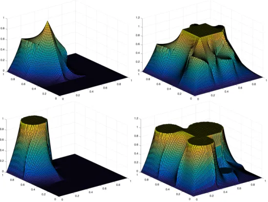
Fig. 3. Domain decomposition into 9 subdomains with coefficient distribution depicted inFig- ure1 with↵= 106. Top Left: MsFEM-D basis function in one vertex; Top Right: Sum of all four MsFEM-D basis functions;Bottom Left: MsFEM-E basis function in one vertex; Bottom Right: Sum of all four MsFEM-E basis functions.
to be found or designed in order to compute the extensions. Therefore, this approach is more general compared to the previous one. However, the energy-minimality prop- erty is, in general, not fulfilled for later Newton iterations. Let us remark that the extensions could be updated using DF(u(k)) in certain Newton steps if the hetero- geneities or nonlinearities changed drastically during the Newton iteration. For our model problems, this was not necessary.
In both approaches, we compute the extensions by(30). Since the matrixAII is block-diagonal, the extensions can be computed concurrently for all subdomains; also cf. (28).
6.2. Interface values. The interface properties (26) and (29) are fulfilled for many classical nodal discretizations; cf.Figure 2for a graphical representation for rect- angular subdomains and piecewise bilinear (Q1) basis functions. For heterogeneous model problems (e.g., Figure 1), multi scale basis functions can significantly di↵er from Lagrangian basis functions while maintaining these properties; cf.Figure 3.
For unstructured grids and domain decompositions, we propose the following two definitions of interface values; since the vertex values are determined by the properties(26), it is only left to define the edge values.
Distance based edge values. As a first option, we consider the edge values intro- duced in [30]. Therefore, let⌫be a vertex,ean adjacent edge, and⌫0 the other vertex
adjacent to the edgee. Then, we set the interface values to
⌘⌫(x) = ||x ⌫||
||x ⌫0||+||x ⌫||
for anyx2e; cf., e.g., [30]. Based on this formula, we compute the values⌘⌫ on each edge adjacent to⌫. On all edges which are not adjacent to⌫, we set⌘⌫ to zero. We denote this variant as MsFEM-D, where “D” indicates that the computation of the edge values is based on distances.
It is easy to see that this choice is not optimal for heterogeneous problem. On straight edges, the values are linear, independent of variations in the coefficient func- tion; seeFigure 3. This is improved in our second variant.
Energy minimal edge values. In contrast to the previous variant, where the edge values are based on distances to the adjacent vertices, we also consider a variant which incorporates the coefficient function. In particular, we propose to use the vertex basis functions of the OS-ACMS coarse space introduced in [28]. The OS- ACMS coarse space is an adaptive coarse space for overlapping Schwarz methods consisting of energy-minimizing basis functions. In particular, the extensions into the interior are computed in the same way as described in subsection 6.1. In addition to the vertex basis functions the OS-ACMS coarse space also contains edge basis functions, which are constructed from the solutions of local generalized eigenvalue problems. However, it turns out that the vertex basis functions alone are already robust for many heterogeneous coefficient distributions; cf., e.g., the heterogeneous problem inFigure 1.
In order to compute the edge values of the OS-ACMS coarse vertex basis function
⌘⌫, let
⌦e=⌦e,1[⌦e,2
where eis an edge and ⌦e,1 and ⌦e,2 are the two subdomains adjacent to e. Then, we compute functions
v⌫,e= arg min
v2V(⌦e) v(⌫0)= ⌫⌫0
|v|2a,⌦e
for all edgeseand define the edge values of⌘⌫ as the edge values of thev⌫,e, i.e.,
⌘⌫|e=v⌫,e|e
We denote this variant as MsFEM-E, where “E” indicates that the computation of the edge values is based on energy minimization.
Obviously, the second variant is more expensive than the first one, however, we can observe that the edge values account for variations in the coefficient functions;
see Figure 3. As a consequence, the MsFEM-E coarse space is more robust (in the sense of linear and nonlinear convergence) for heterogeneous problems; see subsec- tion 8.2.
7. Algorithmic description. In this section, we additionally provide an algo- rithmic point of view of the di↵erent methods. We concentrate on the ASPEN vari- ants, since RASPEN, ASPIN, or RASPIN share the same algorithmic structure. We also provide a comparison with classical Newton-Krylov-Schwarz approaches; seeAl- gorithm 1.
Algorithm 1Newton-Krylov-Schwarz Initu(0)
ComputeF(u(0))
Looponk= 0,1,2, ...until||F(u(k))||/||F(u(0))||< tolouter
ComputeDF(u(k))
Solve iterativelyM 1DF(u(k)) u(k)=M 1F(u(k))
/* Here,M 1 can be any one- or two-level Schwarz preconditioner; We use GMRES to solve the system up to a certain tolerance ) inexact Newton method*/
Updateu(k+1)=u(k) u(k)
/* is the step-length computed, e.g, by a linesearch approach /*
ComputeF(u(k+1)) EndLoop
The usage of di↵erent linear preconditionersM 1inAlgorithm 1changes the lin- ear but not the nonlinear convergence behavior. We consider di↵erent linear one- and two-level Schwarz preconditioners corresponding to their nonlinear relatives described above, e.g., hybrid or additive Schwarz methods with P1, MsFEM-D, or MsFEM-E coarse spaces.
7.1. The ASPEN algorithm. Let nowFXbe a nonlinear function correspond- ing to an arbitrary one- or two-level ASPEN method, e.g.,FX:=FaddorFX :=Fh,2. The ASPEN method then writes as presented inAlgorithm 2.
Algorithm 2ASPEN Initu(0)
ComputeF(u(0))
Looponk= 0,1,2, ...until||F(u(k))||/||F(u(0))||< tolouter
Computeg(k):=FX(u(k)) ComputeDFX(u(k))
Solve iterativelyDFX(u(k)) u(k)=g(k)
/* Here, DFX(u(k)) has already the structure of a Schwarz- preconditioned operator; depending on the nonlinear ASPEN variant;
We use GMRES to solve the system up to a certain tolerance)inexact Newton methods*/
Updateu(k+1)=u(k) u(k)
/* is the step-length computed, e.g, by a linesearch approach /*
ComputeF(u(k+1)) EndLoop
Let us remark that we can also formulate a stopping criterion based onFXinstead of F. We choose the latter option for a better comparability between the di↵erent methods and use the tolerance tolouter = 10 6 in all computations insection 8. In contrast to Newton-Krylov approaches, the evaluation of FX(u(k)) requires the so- lution of nonlinear problems, more precisely, the computation ofTi(u), i= 0, ..., N.
Regardless if a local correction (i > 0) or the coarse correction (i = 0) has to be computed, this is done with Newton’s method and we usetolinner/coarse= 10 3in our computations; seeAlgorithm 3.
Algorithm 3Compute correctiongi:=Ti(u(k)) Initgi(0)= 0
ComputeFi(0) :=RiF(u(k) Pig(0)i )
Looponl= 0,1,2, ... until||Fi(l)||/||Fi(0)||< tolinner/coarse
ComputeDFi(l):=RiDF(u(k) Pig(l)i )Pi
Solve directlyDFi(l) g(l)i =Fi(l)
/* Sparse direct solvers are used here)exact Newton method*/
Updategi(l+1)=gi(l)+ gi(l)
/* is the step-length computed, e.g, by a linesearch approach /*
ComputeFi(l+1):=RiF(u(k) Pigi(l+1)) EndLoop
Setgi:=gi(l+1)
7.2. Evaluation of nonlinear functions. Now, we have stated all ingredients to specify the evaluation of FX(u(k)); see Algorithms 4 to 8. The main di↵erence of the competing methods, i.e., the ordering of local and coarse corrections, can be easily observed in the algorithmic notation.
Algorithm 4Evaluation of one-level ASPEN function g(k):=FA(u(k))
Computelocal correctionsgi:=Ti(u(k)), i= 1, ..., N /*withAlgorithm 3*/
Setg(k):=PN i=1Pigi
Algorithm 5Evaluation of two-level additive ASPEN functiong(k):=Fadd(u(k)) Computelocal correctionsgi:=Ti(u(k)), i= 1, ..., N /*withAlgorithm 3*/
Computecoarse correctiong0:=T0(u(k)) /*withAlgorithm 3*/
Setg(k):=PN
i=1Pigi+P0g0
Let us again remark that we obtain the corresponding RASPEN methods by replacingPi, i= 1, ..., N, byPei, i= 1, ..., N, inAlgorithms 4to8. The corresponding ASPIN or RASPIN methods are finally obtained by replacing DFX in Algorithm 2 by the appropriate approximations suggested insection 4.
7.3. Globalization and inexact solution of the tangential system. We always use an inexact Newton method in the outer loop and solve our preconditioned tangential system using GMRES up to a certain tolerancetolGMRES. In contrast, we use an exact Newton method for the local and coarse corrections, i.e., we solve the tangent problems using sparse direct solves. Without any additional globalization strategy, i.e., by fixing = 1 in Algorithms 1 to 3, global convergence of Newton’s methods is in both cases not guaranteed. Controlling the step-length instead is ben- eficial.
A successful approach to increase the convergence radius of Newton’s method for the solution of an arbitrary nonlinear problem G(x) = 0 is the globally convergent Inexact Newton Backtracking (INB) approach; see [19]. For a given forcing term⌘, the descent condition
(31) ||G(x(k) x(k))||(1 c(1 ⌘))||G(x(k))||
Algorithm 6 Evaluation of two-level hybrid ASPEN function g(k) := Fh,1(u(k)) (coarse correction first)
Computecoarsecorrectiong0:=T0(u(k)) /*withAlgorithm 3*/
Setu˜:=u(k) P0g0
Computelocal correctionsgi:=Ti(˜u), i= 1, ..., N /*withAlgorithm 3*/
Setg(k):=PN
i=1Pigi+P0g0
Algorithm 7 Evaluation of two-level hybrid ASPEN function g(k) := Fh,2(u(k)) (coarse correction second)
Computelocal correctionsgi:=Ti(u(k)), i= 1, ..., N /*withAlgorithm 3*/
Setu˜:=u(k) PN i=1Pigi
Computecoarsecorrectiong0:=T0(˜u) /*withAlgorithm 3*/
Setg(k):=PN
i=1Pigi+P0g0
has to be fulfilled for using a backtracking approach. Here, the constantcis usually small, e.g., c = 10 4, x(k) is the current Newton iterate, and x(k) is the Newton update. The forcing term is initialized with ⌘ =tolGMRES and modified dependent on during the backtracking procedure; see [19] for details. In our computations, we always choosetolGMRES= 10 10 if no globalization strategy is used andtolGMRES = 10 4 if INB is used. The latter choice avoids an oversolving of the linear system and potentially saves GMRES iterations; more elaborate choices of the forcing terms can be found in [20]. To avoid ine↵ectively small step-lengths, we choose 2[0.1,1].
The INB approach can be used without any modification inAlgorithm 1and also in the computation of the local or coarse corrections (Algorithm 3), even though the forcing term is close to zero in the latter case. In contrast to that, enforcing (31) inAlgorithm 2, i.e., enforcing
(32) ||FX(u(k) u(k))||(1 c(1 ⌘))||FX(u(k))||,
requires many evaluations ofFX(u(k) u(k)) for di↵erent , which results in many additional inner and coarse iterations. We propose to replace FX by the original nonlinear function F in (32) as long as u(k) is a descent direction with respect to the energy 12||F(·)||2. If u(k) is not a descent direction, we suggest to completely reject the ASPEN update u(k)and use a Newton-Krylov step instead. This was not necessary in any of our computations.
Since we are essentially interested in the globalization and convergence properties of the di↵erent nonlinear coarse spaces and methods themselves, we do not use INB in general. These properties can be polluted using variable step lengths. Nonetheless, for some of the considered algorithms applied to some of our model problems using INB or an alternative globalization approach is necessary for convergence and we present some results using INB in subsection 8.2. Of course, in practice, we always recommend to use INB or to include an alternative globalization strategy.
8. Numerical results. In this section, we consider the di↵erent nonlinear Schwarz methods described insection 4using standardP1 coarse spaces and the coarse spaces described insection 6. We compare the numbers of outer Newton iterations, inner Newton iterations, coarse Newton iterations, and linear GMRES iterations. We al- ways provide the sum over all outer Newton steps for the inner Newton iterations,
Algorithm 8 Evaluation of symmetric two-level hybrid ASPEN function g(k) :=
Fh(u(k))
Computecoarsecorrectiong0:=T0(u(k)) /*withAlgorithm 3*/
Setu˜:=u(k) P0g0
Computelocal correctionsgi:=Ti(˜u), i= 1, ..., N /*withAlgorithm 3*/
Setuˆ:= ˜u PN i=1Pigi
Computecoarsecorrection ˜g0:=T0(ˆu) /*withAlgorithm 3*/
Setg(k):=PN
i=1Pigi+P0g0+P0g˜0
coarse Newton iterations, and linear GMRES iterations and additionally average over all subdomains for the inner iterations.
8.1. Homogeneous model problem. For a homogeneous coefficient distribu- tion, distance based and the energy minimizing edge values for our MsFEM type coarse spaces yield comparable results; however, the computation of the energy mini- mizing edge values is computationally more demanding. Therefore, we compare only P1 and MsFEM-D coarse spaces in this subsection.
In particular, we cover the following aspects in our numerical investigations for the homogeneous model problem: we compare the di↵erent coarse spaces for the sug- gested two-level RASPEN methods (seeTable 1), we investigate the work distribution in the di↵erent suggested one- and two-level RASPEN methods (see Figure 4), we compare the one- and two-level RASPEN methods to the associated Newton-Krylov- Schwarz approaches for regular and METIS decompositions (seeTable 5), and briefly investigate the use of inexact (RASPIN) methods for regular and METIS domain decompositions (seeTable 2).
Di↵erent coarse spaces. In Table 1, we present a comparison of the P1 coarse space and a MsFEM type coarse space with (distance based edge values) using the two di↵erent energy-minimizing extensions. In general, for the homogeneous model problem, all three coarse spaces show a similar behavior with respect to all metrics.
In all cases, the multiplicative approaches are superior and, for this simple test case, H1-RASPEN shows the best performance. Let us remark that theDK(u(0)) extension is our favorite variant since it can be used for METIS domain decompositions and does not require the availability of a linear surrogate matrixKlin.
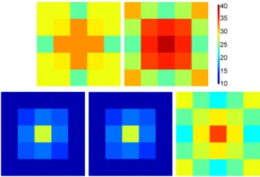
Work distribution. As mentioned before, we average the numbers of inner New- ton iterations over the subdomains in order to estimate the average local work on each subdomain. However, in a parallel implementation, also the work distribution is important, which is dominated by the distribution of inner Newton iterations in non- linear DD methods. To investigate this, we visualize the number of inner iterations for each subdomain for the di↵erent RASPEN approaches in Figure 4 for a regular domain decomposition into 25 subdomains. Here, H-RASPEN and H1-RAPSEN yield the best work distribution. Let us remark that the work imbalance in nonlinear DD methods can also be exploited to save energy. This was discussed in [42] for nonlinear FETI-DP methods as well as for ASPIN, where the nonlinear DD approaches always had a lower power consumption compared with corresponding Newton-Krylov-DD methods.
Regular and METIS domain decompositions. InTable 5, we consider all one- and two-level Newton-Krylov-Schwarz and RASPEN approaches described in this paper using MsFEM type coarse spaces. We do not consider P1 coarse spaces for METIS
Table 1
Comparison of di↵erent coarse spaces (P1 and MsFEM-D with di↵erent extensions described insubsection6.1) for two-level RAPSEN methods for regular domain decompositions; best results for the largest experiments are marked in bold;outer it. gives the number of global Newton iterations;
inner it.gives the number of local Newton iterations summed up over the outer Newton iterations (average over subdomains);coarse it. gives the number of nonlinear iterations on the coarse level summed up over the outer Newton iterations;GMRES it.gives the number of GMRES iterations summed up over the outer Newton iterations.
p-Laplace homogeneous
p= 4;H/h= 16 for regular domains; overlap = 1;
A-RASPEN H-RASPEN
outer inner coarse GMRES outer inner coarse GMRES
N coarse space it. it. (avg.) it. it. (sum) it. it. (avg.) it. it. (sum)
P1 6 31.3 24 98 4 15.2 28 55
9 DK(u(0))-MsFEM-D 6 33.4 27 93 4 17.1 29 52
Klin-MsFEM-D 6 13.6 24 90 3 13.8 21 38
P1 5 26.3 24 109 4 13.4 29 74
25 DK(u(0))-MsFEM-D 6 29.7 29 122 4 13.3 30 72
Klin-MsFEM-D 6 28.5 26 119 3 11.3 22 52
P1 6 29.5 28 150 4 12.1 28 82
49 DK(u(0))-MsFEM-D 6 29.2 28 137 4 12.6 29 80
Klin-MsFEM-D 6 29.7 29 135 3 10.2 23 56
H1-RASPEN H2-RASPEN
P1 4 15.2 17 55 5 27.5 17 78
9 DK(u(0))-MsFEM-D 4 17.1 18 51 5 27.8 15 74
Klin-MsFEM-D 3 13.8 13 39 5 27.2 15 75
P1 4 13.4 18 72 5 25.8 17 101
25 DK(u(0))-MsFEM-D 4 13.3 19 70 5 25.8 18 96
Klin-MsFEM-D 3 11.3 14 53 5 25.9 17 97
P1 4 12.1 18 79 5 25.2 18 110
49 DK(u(0))-MsFEM-D 4 12.6 20 78 5 25.3 17 109
Klin-MsFEM-D 3 10.2 15 56 5 25.3 18 110
domain decompositions because they would require additional coarse triangulations, which are often not available in practice. Especially the hybrid two-level approaches can reduce the number of outer Newton iterations drastically for both types of do- main decompositions. All two-level methods also enable numerical scalability in the linear iterations, which is not the case in one-level RASPEN or one-level Newton- Krylov-Schwarz. Also the nonlinear convergence of the two-level RASPEN methods is superior compared to one-level RASPEN. For the sake of clarity, we will neglect the “A” (additive) and “H2” (hybrid–coarse correction second) variants and concen- trate only on the “H” (hybrid–symmetric) and “H1” (hybrid–coarse correction first) variants in the following sections.
RASPEN vs. RASPIN methods. We compare one- and two-level RASPEN and RASPIN methods for regular and METIS domain decompositions. Whereas the RASPIN method yields better convergence compared to the RASPEN method for the one-level case, the convergence behavior is comparable for the two-level variants;
seeTable 2.
To summarize, considering our metrics, i.e. nonlinear and linear convergence as well as load balance, H1-RASPEN and H-RASPEN perform best. Even for irregular decompositions, our Galerkin product based approaches combined with suitable coarse spaces perform equally well.
8.2. Heterogeneous model problem. For the heterogeneous model problem, i.e.,↵= 103or↵= 106in the yellow circles inFigure 1(left) and↵= 1 elsewhere, we compare Netwon-Krylov-Schwarz and nonlinear one- and two-level Schwarz methods.
Fig. 4. Number of inner Newton iterations per subdomain summed over all outer Newton iterations. Considered problem: Homogeneous4-Laplace with MsFEM-D coarse space andDK(u(0)) extension;H/h= 16 and overlap = 1. From top left to bottom right: one-level RASPEN, A-RASPEN, H-RASPEN, H1-RASPEN, and H2-RASPEN.
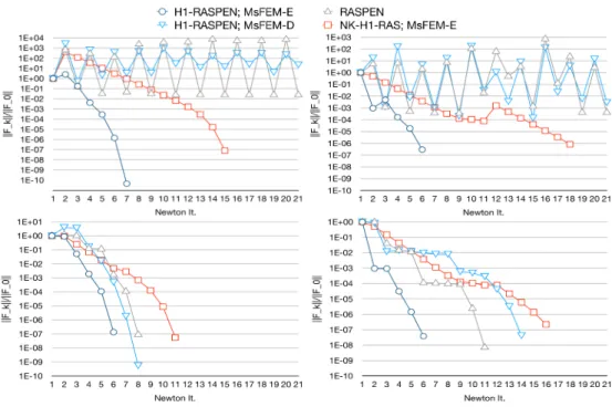
Here, an appropriate coarse space is necessary to obtain good linear convergence and, in case of nonlinear Schwarz methods, also a fast nonlinear convergence. Choosing the MsFEM-E coarse space results in very fast convergence of H1-RASPEN, outper- forming the corresponding Newton-Krylov approach. On the other hand, one-level RASPEN or H1-RASPEN with a P1 or MsFEM-D coarse spaces do not converge within 20 Newton iterations; see Table 3 for the results. Additionally, we provide the convergence history of the outer Newton iteration for four exemplary methods (RASPEN, H1-RASPEN with MsFEM-D and MsFEM-E coarse spaces, and Newton- Krylov-H1-RAS with MsFEM-E coarse space) inFigure 5(top row).
Since a globalization strategy can have a huge impact on the convergence behav- ior, we repeated the same tests using globally convergent INB as described insubsec- tion 7.3. The corresponding results are presented in Table 4 and Figure 5 (bottom row). Now, all considered methods converge within 20 iterations and the number of inner as well as coarse iterations is reduced. Additionally, due to the larger stopping tolerancetolGMRES = 10 4also the number of linear iterations is reduced drastically.
Again, we observe that the choice of an appropriate coarse space is critical for fast convergence of the two-level nonlinear Schwarz method. The H1-RASPEN approach with MsFEM-E coarse space clearly outperforms all other approaches with respect to linear as well as nonlinear convergence. Notably, for the considered heterogeneous model problem, the convergence behavior is even nearly independent of the coefficient jump as well as the globalization strategy; cf.Table 3and Table 4; only the number of GMRES iterations varies due to the di↵erent stopping tolerance.
REFERENCES
[1] J. Aarnes and T. Y. Hou. Multiscale domain decomposition methods for elliptic problems with high aspect ratios. Acta Math. Appl. Sin. Engl. Ser., 18(1):63–76, 2002.
[2] P. Brune, M. Knepley, B. Smith, and X. Tu. Composing scalable nonlinear algebraic solvers.
SIAM Review, 57(4):535–565, 2015.
[3] M. Buck, O. Iliev, and H. Andr¨a. Multiscale finite elements for linear elasticity: Oscillatory boundary conditions. InDomain Decomposition Methods in Science and Engineering XXI,