Technical Report Series
Center for Data and Simulation Science
Alexander Heinlein, Axel Klawonn, Martin Lanser, Janine Weber
Machine Learning in Adaptive FETI-DP - Reducing the Effort in Sampling
Technical Report ID: CDS-2019-19
Available at https://kups.ub.uni-koeln.de/id/eprint/10439
Submitted on December 16, 2019
Reducing the Effort in Sampling
Alexander Heinlein, Axel Klawonn, Martin Lanser, and Janine Weber
1 Introduction
Domain decomposition methods are highly scalable iterative solvers for large lin- ear systems of equations, e.g., arising from the discretization of partial differential equations. While scalability results from a decomposition of the computational do- main into local subdomains, i.e., from a divide and conquer principle, robustness is obtained by enforcing certain constraints, e.g., continuity in certain variables or averages over variables on the interface between neighboring subdomains. These con- straints build a global coarse problem or second level. Nevertheless, the convergence rate of classic domain decomposition approaches deteriorates or even stagnates for large discontinuities in the coefficients of the partial differential equation considered.
As a remedy, to retrieve a robust algorithm, several adaptive approaches to enrich the coarse space with additional constraints obtained from the solution of generalized eigenvalue problems have been developed, e.g., [8, 7, 11, 12, 3, 2]. The eigenvalue problems are in general localized to parts of the interface, e.g., edges or faces. In the present paper, we only consider two-dimensional problems for simplicity and thus only eigenvalue problems on edges. Let us remark that for many realistic coefficient distributions, only a few adaptive constraints on a few edges are necessary to obtain a robust algorithm and thus many expensive solutions of eigenvalue problems can be omitted. Although some heuristic approaches [8, 7] exist to reduce the number of eigenvalue problems, in general, it is difficult to predict a priori which eigenvalue
Alexander Heinlein, Axel Klawonn, and Martin Lanser
Department of Mathematics and Computer Science, University of Cologne, Weyertal 86-90, 50931 Köln, Germany, e-mail: alexander.heinlein@uni-koeln.de, axel.klawonn@uni-koeln.de, martin.lanser@uni-koeln.de, url: http://www.numerik.uni-koeln.de
Center for Data and Simulation Science, University of Cologne, Germany, url: http://www.cds.uni- koeln.de
Janine Weber
Department of Mathematics and Computer Science, University of Cologne, Weyertal 86-90, 50931 Köln, Germany, e-mail: janine.weber@uni-koeln.de, url: http://www.numerik.uni-koeln.de
1
problems are necessary for robustness. In [5], we successfully used a neural network to predict the geometric location of necessary constraints in a preprocessing step, i.e., to automatically make the decision whether or not we have to solve a specific eigenvalue problem. Additionally, we discussed the feasibility of randomly, and thus automatically generated training data in [4]. In the present paper, we extend the results given in [4] by providing also results for linear elasticity problems.
Both in [5] and [4], we use samples of the coefficient function as input data for the neural network. In particular, in case of regular decompositions, the resulting sampling points cover the complete neighboring subdomains for a specific edge.
Even though the training of the neural network as well as the generation of the training data can be performed in an offline-phase, we aim to further optimize the complexity of our approach by reducing the size of the input data by using fewer sampling points; see also Fig. 1 for an illustration. In particular, for the first time, we only compute sampling points for slabs of varying width around a specific edge between two subdomains. Since our machine learning problem, in principle, is an image classification task, this corresponds to the idea of using only a fraction of pixels of the original image as input data for the neural network. We show numerical results for linear elasticity problems in two dimensions. As in [5], we focus on a certain adaptive coarse space for the FETI-DP (Finite Element Tearing and Interconnecting - Dual Primal) algorithm [11, 12].
2 Linear Elasticity and an Adaptive FETI-DP Algorithm
In our numerical experiments, we exclusively consider linear elasticity problems.
We denote byu:Ω→R2the displacement of an elastic body, which occupies the domainΩ in its undeformed state. We further denote by f a given volume force and byga given surface force onto the body. The problem of linear elasticity then consists in finding the displacementu∈H10(Ω, ∂ΩD), such that
∫
Ω
Gε(u):ε(v)dx+∫
Ω
Gβdivudivvdx=hF,vi
for allv∈H10(Ω, ∂ΩD)for given material functionsG:Ω→Randβ:Ω→Rand the right-hand side
hF,vi=∫
Ω
fTvdx+∫
∂ΩN
gTvdσ.
The material parametersG and βdepend on the Young modulus E > 0 and the Poisson ratio ν ∈ (0,1/2) given by G = E/(1+ν) and β = ν/(1−2ν). Here, we restrict ourselves to compressible linear elasticity; hence, the Poisson ratioνis bounded away from 1/2.
In the present article, we apply the proposed machine learning based strategy to an adaptive FETI-DP method, which is based on a nonoverlapping domain de-
composition of the computational domainΩ. Here, we decomposeΩintoNregular subdomains of widthHand discretize each subdomain by finite elements of width h. For simplicity, we assume matching nodes on the interface between subdomains.
Due to space limitations, we do not explain the standard FETI-DP algorithm in detail.
For a detailed description, see, e.g., [10]. Let us just note that we enforce continuity in all vertices of all subdomains to define an initial coarse space.
As already mentioned in section 1, for arbitrary and complex material distribu- tions, e.g., a highly varying Young modulusE, using solely primal vertex constraints is not sufficient to guarantee a robust condition number bound. Thus, additional adap- tive constraints, typically obtained from the solution of local generalized eigenvalue problems, are used to enrich the coarse space and retrieve robustness.
The central idea of the adaptive FETI-DP algorithm [11, 12] is to solve local generalized eigenvalue problems for all edges between two neighboring subdomains.
For a description of the local edge eigenvalue problems and the resulting enforced coarse constraints, see [11, 12]. In a parallel implementation, the set-up, e.g., the computation of local Schur complements, and the solution of the local eigenvalue problems take up a significant amount of the total time to solution. To reduce the set-up cost without losing robustness, a precise a priori prediction of all edges, where an eigenvalue problem is useful, is necessary; see section 3 for a description of our machine learning based approach. Let us remark, that the additional adaptive constraints are implemented in FETI-DP using a balancing preconditioner. For a detailed description of projector or balancing preconditioning, see [9, 6].
3 Machine Learning for Adaptive FETI-DP
Our approach (ML-FETI-DP) is to train a neural network to automatically make the decision whether an adaptive constraint needs to be enforced or not on a specific edge to retain the robustness of the adaptive FETI-DP algorithm. This corresponds to a supervised machine learning technique.
Sampling strategy and neural network:More precisely, we use a dense feedfor- ward neural network, i.e., a multilayer perceptron, to make this decision. For more details on multilayer perceptrons, see, e.g., [13, 1, 14]. As in [5], we use samples, i.e., function evaluations of Young’s modulus within the two subdomains adjacent to an edge, as input data for our neural network. Note that our sampling approach is independent of the finite element discretization. In particular, we assume that the sampling grid resolves all geometrical details of the coefficient function or the ma- terial distribution. The output of our neural network is the classification whether an adaptive constraint has to be included for a specific edge or not. Our neural network consists of three hidden layers with 30 neurons for each hidden layer. We use the ReLU activation function for all hidden layers and a dropout rate of 20%. See [5] for more details on the machine learning techniques and the preparation of data.
Training data sets: For the numerical results presented here, we train on two regular subdomains sharing a straight edge. In general, also irregular domain decom-
positions can be considered; see [5]. As in [4], we use different sets of coefficient distributions to generate different sets of training data for the neural network. For the first set of training data, we use a total of 4,500 configurations varying the co- efficient distributions as presented in Fig. 2. We set the Poisson ratio νconstantly and just vary the Young modulusE. The coefficient distributions in Fig. 2 are varied in size, orientation and location to obtain the full set of training data. We refer to this set of training data assmart data; see also [4]. We further consider a randomly generated training data set. In particular, we use the same training sets as in [4] but now additionally provide results for linear elasticity problems. Note that completely randomized coefficient distributions lead to insufficient accuracies and too many false negatives; see [4] for details. Instead, we explicitly control the ratio of high coefficients as well as the distributions of the coefficients to a certain degree by ran- domly generating either horizontal or vertical stripes of a maximum length of four or eight pixels, respectively; see Fig. 3. We refer to this second set of training data as random dataand we also consider combinations of both, thesmartandrandom data sets. For more technical details on the construction of the data sets, we refer to [4].
Ωi Ωj
Ei j
... ...
... ...
Input layer
Hidden layers
Output layer ρ(x1)
ρ(x2)
ρ(xk)
ρ(xM)
use evp?
Fig. 1 Sampling of the coefficient function; white color corresponds to a low coefficient and red color to a high coefficient. In this representation, the samples are used as input data for a neural network with two hidden layers. Only sampling points from slabs around the edge are chosen.
Sampling strategy on slabs:We now describe how we reduce the number of sampling points used as input data for the neural network. In [5], the computed sampling grid covers both neighboring subdomains of an edge entirely - at least in case of a regular domain decomposition. Let us remark that in case of irregular domain decompositions, our sampling strategy might miss small areas further away from the edge; see, e.g., [5, Fig. 4]. However, this does not affect the performance of our algorithm. Although the preparation of the training data as well as the training of the neural network can be performed in an offline-phase, we try to generate the training data as efficient and fast as possible. For all sampling points, we need to determine the corresponding finite element as well as to evaluate the coefficient function for the respective finite element. Therefore, there is clearly potential to save resources and compute time in the training as well as in the evaluation phase by reducing the number of sampling points used as input data for the neural network.
In general, the coefficient variations close to the edge are the most relevant, i.e., the most critical for the condition number bound of FETI-DP. Therefore, to reduce the
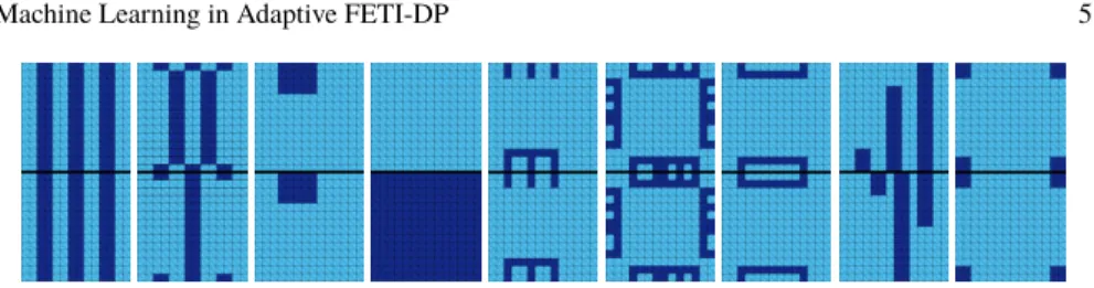
Fig. 2 Nine different types of coefficient functions used for training and validation of the neural network. The inclusions, channels, boxes, and combs with high coefficient are displaced, modified in sized, and mirrored with respect to the edge in order to generate the completesmart dataset.
Fig. 3 Examples of three different coefficient functions taken from therandom dataset obtained by using the same randomly generated coefficient for a horizontal (left) or vertical (middle) stripe of a maximum length of four finite element pixels, as well as by pairwise superimposing (right).
total number of sampling points in the sampling grid, reducing the density of the grid points with increasing distance to the edge is a natural approach. More drastically, one could exclusively consider sampling points in a neighborhood of the edge, i.e., on slabs next to the edge. We consider the latter approach here; see also Fig. 1 for an illustration of the sampling points inside slabs.
To generate the output data necessary to train the neural network, we solve the eigenvalue problems as described in [11, 12] for all the aforementioned training and validation configurations. Concerning the classification of the edges, we use both a two-class and a three-class classification approach. For the two-class classification, we only distinguish between edges of class 0 and class 1. By class 0 we denote edges for which no additional constraints are necessary for a robust algorithm, and by class 1 edges where at least one constraint is required. For the three-class classification, we further differentiate between class 1 and class 2. In this case, we assign only edges to class 1, where exactly one additional constraint is necessary, and assign all other edges, for which more than one constraint is necessary, to class 2.
4 Numerical Results
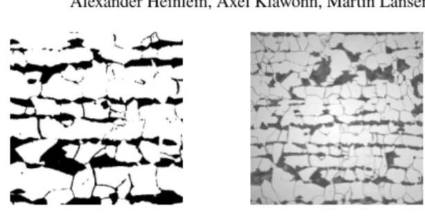
We first provide results for some microsection problems, i.e., linear elasticity prob- lems with a material distribution as shown in Fig. 4 (left). We considered the different training setssmart data,random data, and a combination of both; see Table 1. Here, we exclusively use the approach of sampling on the complete subdomains. Since training with thesmart dataset seems to be the best choice for this specific example, we exclusively use this data set in the following investigations with slabs of different
Fig. 4 Left:Subsection of a microsection of a dual-phase steel obtained from the image on the right.
We considerE=1e3 in the black part andE=1 elsewhere.Right:Complete microsection of a dual-phase steel. Right image: Courtesy of Jörg Schröder, University of Duisburg-Essen, Germany, orginating from a cooperation with ThyssenKruppSteel.
width. Additionally, using the ML thresholdτ=0.45 for the two-class classification or τ = 0.4 for the three-class classification, respectively, leads to the most robust results when sampling on the complete subdomains. We therefore focus on these thresholds in the following discussion.
We compare the performance of the original sampling approach introduced in [5]
to sampling in parts of each subdomain of width H, i.e., in one half and in one quarter (see also Fig. 1). We also consider the extreme case, i.e., sampling only inside minimal slabs of the width of a single finite element. For the training data, both sampling inH/2 andH/4 leads to accuracy values which are only slightly lower than for the full sampling approach (see Table 2). In particular, we get slightly higher false positive values, especially for the three-class classification. For the extreme case of sampling only in slabs of widthh, i.e., using slabs with the minimal possible width in terms of finite elements, the accuracy value drops from 92.8% for the three- class model to only 68.4% for the thresholdτ =0.4. Note that we did not observe a significant improvement for this sampling strategy for more complex network architectures. Thus, it is questionable if the latter sampling approach still provides a reliable machine learning model. For the microsection problem, sampling in slabs of width H/2 andH/4 results in robust algorithms for both the two-class and the three-class model when using the ML thresholdτ =0.45 orτ =0.4, respectively;
see Tables 3 and 4. For all these approaches, we obtain no false negative edges, which are critical for the convergence of the algorithm. However, the use of fewer sampling points results in more false positive edges and therefore in a larger number of computed eigenvalue problems. When sampling only in slabs of widthh, we do not obtain a robust algorithm for the microsection problem for neither the two-class nor the three-class classification. This is caused by the existence of a relatively high number of false negative edges.
Let us summarize that reducing the effort in the training and evaluation of the neural network by reducing the size of the sampling grid still leads to a robust algorithm for our model problems. Nevertheless, the slab width cannot be chosen too small and enough finite elements close to the edge have to be covered by the sampling grid.
Alg. T-Data τ cond it evp fp fn acc
standard - - - >300 0 - - -
adaptive - - 79.1 ( 92.8) 87.4 (91) 112.0 (112) - - -
ML S 0.5 9.3e4 (1.3e5) 92.2 (95) 44.0 ( 56) 2.2 ( 3) 2.4 (3) 0.96 (0.95) S 0.45 79.1 ( 92.8) 87.4 (91) 48.2 ( 61) 4.8 ( 7) 0 (0)0.95 (0.93) R1 0.45 1.7e3 (2.1e4) 90.4 (91) 53.6 ( 57) 13.4 (16) 0.8 (1) 0.87 (0.86) R2 0.45 79.1 ( 92.8) 87.4 (91) 52.8 ( 57) 11.6 (12) 0 (0) 0.90 (0.87) SR 0.45 79.1 ( 92.8) 87.4 (91) 50.6 ( 61) 8.8 (10) 0 (0) 0.92 (0.90) Table 1 Comparison of standard FETI-DP, adaptive FETI-DP, and ML-FETI-DP for aregular domain decompositioninto 8×8 subdomains withH/h =64,linear elasticity, thetwo-class model, and 10 different subsections of the mircosection in Fig. 4 (right). We denote by ’S’ the training set of 4,500smart data, by ’R1’ and ’R2’ a set of 4,500 and 9,000random data, respectively, and by ’SR’ the combination of 4,500smartand 4,500random data. We show the ML-threshold (τ), the condition number (cond), the number of CG iterations (it), the number of solved eigenvalue problems (evp), the number of false positives (fp), the number of false negatives (fn), and the accuracy in the classification (acc). We define the accuracy (acc) as the number of true positives and true negatives divided by the total number of training configurations. We show the average values as well as the maximum values (in brackets).
two-class three-class
training configurationτ fp fn acc τ fp fn acc full sampling 0.45 8.9% 2.7% 88.4% 0.4 5.2% 2.0% 92.8%
0.5 5.5% 5.6% 88.9% 0.5 3.3% 3.3% 93.4%
sampling inH/2 0.45 8.0% 2.6% 89.4% 0.4 9.6% 4.3% 86.1%
0.5 5.9% 4.0% 90.1% 0.5 7.4% 5.0% 87.6%
sampling inH/4 0.45 8.2% 2.7% 89.1% 0.4 10.4% 3.9% 85.7%
0.5 5.7% 4.5% 89.8% 0.5 8.1% 4.8% 87.1%
sampling inh 0.45 20.8% 7.5% 71.7% 0.4 22.4% 9.2% 68.4%
0.5 15.4% 12.9% 72.3% 0.5 15.0% 15.3% 69.7%
Table 2 Results on the complete training data set forlinear elasticity; the numbers are averages over all training configurations. See Table 1 for the column labelling.
Model Problem Algorithm τ cond it evp fp fn acc standard - ->300 0 - - -
Microsection adaptive - 84.72 89 112 - - -
Problem ML, full sampling 0.5 9.46e4 91 41 2 2 0.96 ML, full sampling 0.45 84.72 89 46 5 0 0.95 ML, sampling inH/2 0.45 84.72 89 47 6 0 0.95 ML, sampling inH/4 0.45 85.31 90 48 7 0 0.94 ML, sampling inh0.45 10.9e5 137 50 19 10 0.74
Table 3 Comparison of standard FETI-DP, adaptive FETI-DP, and ML-FETI-DP for aregular domain decompositioninto 8×8 subdomains withH/h =64,linear elasticity, thetwo-class model, and the microsection subsection in Fig. 4 (left). See Table 1 for the column labelling.
References
1. I. Goodfellow, Y. Bengio, and A. Courville.Deep learning, volume 1. MIT press Cambridge, 2016.
Model Problem Algorithm τ cond it evp e-avg fp fn acc standard - ->300 0 - - - -
Microsection adaptive - 84.72 89 112 - - - -
Problem ML, full sampling 0.5 274.73 101 15 31 3 2 0.96 ML, full sampling 0.4 86.17 90 22 24 6 0 0.95 ML, sampling inH/2 0.4 85.29 90 25 26 9 0 0.92 ML, sampling inH/4 0.4 85.37 90 25 27 10 0 0.92 ML, sampling inh0.4 2.43e4 111 27 52 29 7 0.68 Table 4 Comparison of standard FETI-DP, adaptive FETI-DP, and ML-FETI-DP for aregular domain decompositioninto 8×8 subdomains withH/h=64,linear elasticity, thethree-class model, and the microsection subsection in Fig. 4 (left). See Table 1 for the column labelling. Here, e-avgdenotes an approximation of the coarse constraints for edges in class 1, see also [5].
2. A. Heinlein, A. Klawonn, J. Knepper, and O. Rheinbach. An adaptive GDSW coarse space for two-level overlapping Schwarz methods in two dimensions. 2017. Accepted for publication to the Proceedings of the 24rd International Conference on Domain Decomposition Methods, Springer Lect. Notes Comput. Sci. Eng.
3. A. Heinlein, A. Klawonn, J. Knepper, and O. Rheinbach. Multiscale coarse spaces for overlap- ping Schwarz methods based on the ACMS space in 2D.Electronic Transactions on Numerical Analysis (ETNA), 48:156–182, 2018.
4. A. Heinlein, A. Klawonn, M. Lanser, and J. Weber. Machine Learning in Adaptive FETI-DP - A Comparison of Smart and Random Training Data. 2018. TR series, Center for Data and Simulation Science, University of Cologne, Germany, Vol. 2018-5. http://kups.ub.uni- koeln.de/id/eprint/8645. Accepted for publication in the proceedings of the International Con- ference on Domain Decomposition Methods 25, Springer LNCSE, May 2019.
5. A. Heinlein, A. Klawonn, M. Lanser, and J. Weber. Machine Learning in Adaptive Domain Decomposition Methods - Predicting the Geometric Location of Constraints. SIAM J. Sci.
Comput., 41(6):A3887–A3912, 2019.
6. M. Jarošová, A. Klawonn, and O. Rheinbach. Projector preconditioning and transformation of basis in FETI-DP algorithms for contact problems.Math. Comput. Simulation, 82(10):1894–
1907, 2012.
7. A. Klawonn, M. Kühn, and O. Rheinbach. Adaptive coarse spaces for FETI-DP in three dimensions.SIAM J. Sci. Comput., 38(5):A2880–A2911, 2016.
8. A. Klawonn, M. Kühn, and O. Rheinbach. Adaptive FETI-DP and BDDC methods with a generalized transformation of basis for heterogeneous problems.Electron. Trans. Numer. Anal., 49:1–27, 2018.
9. A. Klawonn and O. Rheinbach. Deflation, projector preconditioning, and balancing in iterative substructuring methods: connections and new results. SIAM J. Sci. Comput., 34(1):A459–
A484, 2012.
10. A. Klawonn and O. B. Widlund. Dual-primal FETI methods for linear elasticity.Comm. Pure Appl. Math., 59(11):1523–1572, 2006.
11. J. Mandel and B. Sousedík. Adaptive selection of face coarse degrees of freedom in the BDDC and the FETI-DP iterative substructuring methods. Comput. Methods Appl. Mech. Engrg., 196(8):1389–1399, 2007.
12. J. Mandel, B. Sousedík, and J. Sístek. Adaptive BDDC in three dimensions. Math. Comput.
Simulation, 82(10):1812–1831, 2012.
13. A. Müller and S. Guido. Introduction to Machine Learning with Python: A Guide for Data Scientists. O’Reilly Media, 2016.
14. S. Shalev-Shwartz and S. Ben-David.Understanding Machine Learning. Cambridge University Press, 2014.