Technical Report Series Center for Data and Simulation Science

Center for Data and Simulation Science

Alexander Heinlein, Axel Klawonn, Jascha Knepper, Oliver Rheinbach, Olof B. Widlund

Adaptive GDSW coarse spaces of reduced dimension for overlapping Schwarz methods

Technical Report ID: CDS-2020-4

Available at https://kups.ub.uni-koeln.de/id/eprint/12113

Submitted on September 4, 2020

ALEXANDER HEINLEIN^∗†, AXEL KLAWONN^∗†, JASCHA KNEPPER^∗, OLIVER 3

RHEINBACH^‡, AND OLOF B. WIDLUND^§ 4

Abstract. A new reduced dimension adaptive GDSW (Generalized Dryja-Smith-Widlund) 5 overlapping Schwarz method for linear second-order elliptic problems in three dimensions is in- 6 troduced. It is robust with respect to large contrasts of the coefficients of the partial differential 7 equations. The condition number bound of the new method is shown to be independent of the co- 8 efficient contrast and only dependent on a user-prescribed tolerance. The interface of the nonover- 9 lapping domain decomposition is partitioned into nonoverlapping patches. The new coarse space is 10 obtained by selecting a few eigenvectors of certain local eigenproblems which are defined on these 11 patches. These eigenmodes are energy-minimally extended to the interior of the nonoverlapping 12 subdomains and added to the coarse space. By using a new interface decomposition the reduced 13 dimension adaptive GDSW overlapping Schwarz method usually has a smaller coarse space than 14 existing GDSW and adaptive GDSW domain decomposition methods. A robust condition number 15 estimate is proven for the new reduced dimension adaptive GDSW method which is also valid for 16 existing adaptive GDSW methods. Numerical results for the equations of isotropic linear elasticity 17 in three dimensions confirming the theoretical findings are presented.

18

Key words. domain decomposition, multiscale, GDSW, overlapping Schwarz, adaptive coarse 19 spaces, reduced dimension

20

AMS subject classifications. 65F08,65F10,65N55,68W10 21

1. Introduction. Successful domain decomposition preconditioners for solv-

22

ing elliptic problems all require at least one global, coarse-level component in order

23

to perform satisfactorily if the number of subdomains, into which the given domain

24

has been decomposed, is relatively large. The design and analysis of these coarse

25

components is central in most studies in this field given that they require global

26

communication if the algorithms are implemented on distributed or parallel com-

27

puting systems. In order to avoid creating a bottleneck, it is very important to keep

28

the dimension of the related coarse space small.

29

In recent years, substantial progress has been possible by the development of

30

algorithms which adaptively design the coarse space at a cost of solving local gen-

31

eralized eigenvalue problems. In this paper, we will focus on a particular family

32

of domain decomposition algorithms, the two-level overlapping Schwarz methods,

33

which use one coarse-level component in addition to local components each of which

34

is defined on a subdomain which is part of an overlapping decomposition. We note

35

that the use of adaptively designed coarse spaces has been very successful even with

36

problems with very irregular coefficients; this is clearly demonstrated by examples

37

in section 14 of this paper.

38

The robustness of many coarse spaces for arbitrary coefficient functions is ob-

39

tained by using local generalized eigenvalue problems to adaptively enrich the coarse

40

spaces with suitable basis functions; see, e.g., [14, 10, 41, 15, 20, 13]. These ap-

41

proaches differ, e.g., in the sizes of the eigenvalue problems, the coarse space di-

42

mensions, the class of problems considered, and their parallel efficiency. We also

43

∗Department of Mathematics and Computer Science, University of Cologne, Weyertal 86- 90, 50931 Köln, Germany,{alexander.heinlein, axel.klawonn, jascha.knepper}@uni-koeln.de,http:

//www.numerik.uni-koeln.de

†Center for Data and Simulation Science, University of Cologne, 50931 Köln, Germany,http:

//www.cds.uni-koeln.de

‡Institut für Numerische Mathematik und Optimierung, Fakultät für Mathematik und Informatik, Technische Universität Freiberg, Akademiestr. 6, 09599 Freiberg, oliver.rhein- bach@math.tu-freiberg.de,http://www.mathe.tu-freiberg.de/nmo/mitarbeiter/oliver-rheinbach

§Department of Mathematics, Courant Institute, 251 Mercer Street, New York, NY 10012, USA,widlund@cims.nyu.edu,https://cs.nyu.edu/faculty/widlund

mention success with adaptive coarse spaces for nonoverlapping domain decompo-

44

sition methods; see, e.g., [2, 34, 35, 42, 37, 31, 33, 38, 30, 32, 36].

45

Two-level overlapping Schwarz algorithms were first developed with coarse spa-

46

ces based on a coarse triangulation of the domain and with subdomains obtained

47

by adding one or a few layers of fine elements to each coarse mesh element, see [43,

48

Chapter 3]. On the other hand, the iterative substructuring algorithms, developed

49

for decompositions of the domain into nonoverlapping subdomains, were immedi-

50

ately available for quite irregular subdomains such as those that can be obtained by

51

a mesh partioner such as METIS [29]; see [43, Chapter 4, 5, and 6]. The iterative

52

substructuring algorithms have been very successful but they cannot be used unless

53

submatrices associated with the subdomains are available instead of just a fully

54

assembled stiffness matrix. This was a main reason why a new family of overlap-

55

ping Schwarz algorithms was developed, known as the GDSW methods (generalized

56

Dryja–Smith–Widlund), which borrow their coarse components from [43, Algorithm

57

5.16]. These ideas were first developed in [5, 6]. The elements of these coarse spaces

58

are defined by their values on the interface between the subdomains with values

59

in the interiors defined by energy-minimizing extensions. These algorithms were

60

further developed for almost incompressible elasticity in two papers [7, 8]; in the

61

second paper the dimension of the coarse spaces was considerably decreased; see

62

also [23, 16, 24, 25, 17, 22, 26] for further developments.

63

In this paper, we present an approach of constructing adaptive coarse spaces

64

for the two-level overlapping Schwarz method [40, 43] based on the adaptive GDSW

65

(AGDSW) coarse space of [21]. In particular, our focus is on one new coarse space –

66

the reduced dimension adaptive GDSW (RAGDSW) coarse space – and the reduc-

67

tion of the coarse space dimension. A proof of a condition number estimate, which

68

is independent of heterogeneities of the coefficient functions, is given in sections 10

69

and 11. We note that this proof is based on a more general decomposition of the

70

interface than the one in [21]; it applies to both, the original AGDSW and the new

71

RAGDSW coarse space. Supporting numerical results are presented in section 14.

72

In our adaptive algorithms, a user prescribed tolerance directly controls the

73

condition number of the preconditioned operator and, if this tolerance is chosen as

74

zero, adaptive GDSW is identical to GDSW and reduced dimension adaptive GDSW

75

is identical to reduced dimension GDSW, the latter being a variant of GDSW defined

76

on a specific interface partition of the domain decomposition; cf. section 8.

77

We note that our reduced dimension GDSW coarse space differs from the re-

78

duced dimension GDSW coarse spaces in [9]. However, they share the same core

79

idea: GDSW and AGDSW use basis functions associated with coarse nodes, edges,

80

and faces while the coarse spaces in [9], reduced dimension GDSW, and reduced

81

dimension adaptive GDSW use basis functions associated only with subdomain

82

vertices. Generally, this leads to a reduction in the coarse space dimension. See

83

also [8, 4, 27, 18] for reduced dimension GDSW coarse spaces.

84

We note that many other approaches to constructing coarse spaces exist. Some

85

borrow the idea from the multiscale finite element method (MsFEM) [28, 12] and

86

use basis functions of that type in the coarse space; c.f. [1, 3, 15, 20, 13]. However,

87

the coarse spaces in this paper are not based on MsFEM functions.

88

The outline of the paper is as follows: In section 2, we introduce our model

89

problem followed by the definition of the two-level additive overlapping Schwarz

90

methods in section 3. In the following five sections, we introduce four families of

91

GDSW algorithms. In section 9, we give a quite general description of adaptive

92

GDSW coarse spaces which covers both adaptive GDSW and reduced dimension

93

adaptive GDSW; see also section 12 for a variant which is computationally cheaper,

94

easier to implement and more efficient in a parallel implementation. In sections 10

95

and 11, we derive a condition number estimate for our new reduced dimension

96

adaptive GDSW preconditioner. In section 13, we address questions that may arise

97

Table 1

Reference table for some definitions used in this paper (in order of their appearance).

Description of coarse spaces (sections4–8)

x^h finite element node section 4

P nonoverlapping partition of the interface section 4 Ωξ union of the closure of the subdomains adjacent to aξ∈ P section 5 {ξi}ⁿ_i=1^ξ partitioning of aξ∈ P into nodal equivalence classes

structured mesh, structured domain decomposition eq.(7.1) unstructured mesh, unstructured domain decomposition section 8 n(x^h) index set of subdomains which containx^h eq.(8.1)

Theory (sections9–11)

n^ξ index set of subdomains adjacent to aξ∈ P eq.(9.1)

zξ G(·) extension by zero fromξtoG eq.(9.2)

X^h(ξ) X^h(ξ) :={v:ξ→R³} section 9

Hξ Ω_ξ(·) energy-minimal extension fromξtoΩξ eq.(9.3) c_ξ(u, v) c_ξ(u, v) :=Pn_ξ

i=1c_ξi(u, v) eq.(9.4)

cξ_i(u, v) cξ_i(u, v) :=aΩ_ξi(zξ_i Ω_ξi(u), zξ_i Ω_ξi(v)) eq.(9.5)

kuk²_cξ kuk²_cξ:=cξ(u, u) eq.(9.6)

Πξw Πξ:=P

λ_k,ξ≤tol_ξcξ(w, vk,ξ)vk,ξ eq.(10.1) ΠPw ΠPw:=P

ξ∈PΠξw eq.(10.1)

|u|_d

ξ |u|_d

ξ:=p

dξ(u, u), dξ(·,·) :=aΩ_ξ(Hξ Ω_ξ(·),Hξ Ω_ξ(·)) eq.(10.2)

|u|_a(B) |u|_a(B):=p

aB(u, u) eq.(10.3)

Cτ max. number of vertices of a finite element Lemma 11.2

P(Ω_i) ξ∈ Padjacent to subdomaini eq.(11.1)

N^ξ max. number ofξ∈ Padjacent to a subdomain eq.(11.1)

tolP tolP:= minξ∈Ptolξ Lemma 11.2

N_ec,P N_ec,P:=S

ξ∈P{ξ_i, i= 1, . . . , nξ} eq.(11.2) C measure for theP-connectivity of the domain decomposition eq.(11.3)

about the implementation due to the encounter of singular matrices for certain ex-

98

tension operators described in section 9. Finally, in section 14, we present numerical

99

results for a selection of coefficient functions.

100

For the reader’s convenience, an overview of some definitions is given in Table 1.

101 102

2. Linear elasticity. We will consider a variational formulation of the equa-

103

tions of compressible linear elasticity: Find u ∈ H

₀¹

(Ω)

³

such that

104

(2.1) a

_Ω

(u, v) = L(v) ∀v ∈ H

₀¹

(Ω)

³

105

,

where Ω ⊂ R

³

is a polyhedral domain and

106

a

_Ω

(u, v) :=

Z

Ω

2µ(x)

ε(u(x)) : ε(v(x)) dx +

Z

Ω

λ(x)

div(u(x)) div(v(x))

107

dx,

L(v) :=

Z

Ω

f (x) · v(x) dx.

108109

The Lamé parameters 0 < λ(x), µ(x) : R

³

→ R are scalar coefficient functions,

110

f ∈ L

²

(Ω)

³

111

,

ε(u) :=

¹₂

∇u + ∇u

T

112

and

113

A : B := tr(A

^T

B) =

d

X

i,j=1

A

_ij

B

_ij

.

114

for any matrices A, B ∈ R

^3×3

.

115

We will consider problems with a highly heterogeneous Young modulus E : Ω →

116

R, 0 < E

_min

≤ E(x) ≤ E

_max

, and a positive Poisson ratio ν, bounded away, from

117

above, by 1/2 , and we define the Lamé parameters by

118

λ(x) := E(x)ν (1 + ν)(1 − 2ν) ,

119

µ(x) := E(x) 2(1 + ν) .

120121

The algorithms described in this paper can also be applied to other linear,

122

second-order elliptic problems including those in two dimensions.

123

Let τ

h

:= τ

h

(Ω) be a finite element discretization of Ω. We will use a conforming

124

space V

^h

(Ω) of piecewise linear or trilinear finite elements on this mesh, and for

125

simplicity assume that the Lamé parameters are constant on each element T ∈ τ

h

.

126

We will use the conjugate gradient method preconditioned by two-level over-

127

lapping Schwarz methods to solve the resulting linear system Ku = b.

128

For completeness, we note that the Dirichlet boundary condition has been in-

129

corporated into the global stiffness matrix by setting those rows and columns of K

130

to unit vectors that correspond to Dirichlet boundary nodes.

131

3. Two-level overlapping Schwarz methods. We will now introduce the

132

two-level Schwarz algorithms, mostly following [43, Chapter 2.2]. The different

133

variants considered in this paper will differ in the coarse space chosen; the design of

134

the coarse space is the main issue in this study and many other studies of algorithms

135

of this kind. In the next five sections, we will introduce four different variants. In

136

section 12, we also explore alternatives that decrease the costs of using the two

137

algorithms which use adaptive choices of their coarse spaces.

138

We partition the domain Ω into N nonoverlapping subdomains Ω

i

with a max-

139

imum diameter H , each a union of finite elements, and denote the corresponding

140

interface by Γ := S

i6=j

(∂Ω

_i

∩ ∂Ω

_j

) \ ∂Ω . We extend each subdomain Ω

_i

by k lay-

141

ers of finite elements to obtain an overlapping domain decomposition {Ω

⁰_i

}

^N_i=1

and

142

introduce subspaces V

i

:= V

^h

(Ω

⁰_i

), i ∈ 1, . . . , N , of finite element functions that

143

vanish on ∂Ω

⁰_i

and in the complement of Ω

⁰_i

.

144

Associated with each such subdomain is a restriction operator R

i

: V

^h

(Ω) → V

i 145

and an extension operator R

^T_i

: V

i

→ V

^h

. Furthermore, for any global coarse space

146

V

0

⊂ V

^h

, we define a linear interpolation operator R

0

: V

^h

→ V

0

, where each of

147

the columns of the matrix R

^T₀

represents a coarse basis function defined on the fine

148

mesh τ

h

.

149

We will use exact solvers for all the subspaces defined in terms of bilinear forms

150

on V

_i

, i ∈ {0, 1, . . . , N }, given by

151

˜

a

i

(u

i

, v

i

) = a

Ω

R

^T_i

u

i

, R

^T_i

v

i

∀u

i

, v

i

∈ V

i

;

152153

cf. [43, Chapter 2.2]. The associated matrices are given by K

_i

= R

_i

KR

^T_i

, i =

154

0, 1, . . . , N . The additive one-level Schwarz preconditioned operator is given by

155

P

_OS-1

= P

N

i=1

R

^T_i

K

_i⁻¹

R

i

K , and that of the additive two-level Schwarz operator by

156

P

_OS-2

= R

^T₀

K

₀⁻¹

R

₀

K + P

_OS-1

.

157

4. The GDSW preconditioner. In what follows, x

^h

will denote a finite

158

element node. Those on the interface form the set Γ

^h

:= {x

^h

∈ Γ} . A key ingredient

159

of each of our coarse spaces is a partition P of Γ

^h

into disjoint interface components

160

ξ

^h

⊂ Γ

^h

, s.t.

161

Γ

^h

= [

ξ^h∈P

ξ

^h

.

162

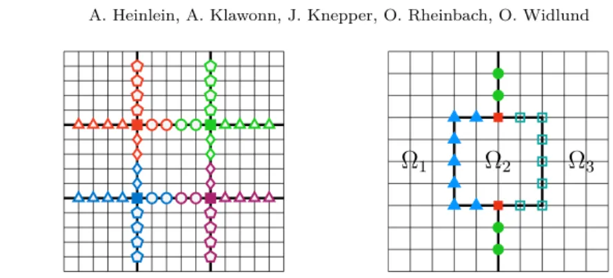
(A)GDSW partitioning GDSW vertex function GDSW edge function

R(A)GDSW partitioning RGDSW basis function

Fig. 1. Left: Decomposition of the interface Γ^h. Top-Left: Decomposition of Γ^h into 16 components: 4 vertices and 12 edges (with 4 nodes each) as used in the GDSW and adaptive GDSW method. Bottom-Left: Decomposition of Γ^hinto 4 components as used in the reduced dimension GDSW and reduced dimension adaptive GDSW methods. Right: Corresponding coarse functions for a two-dimensional diffusion problem are shown on the right for GDSW (top) and RGDSW (bottom). Homogeneous Dirichlet boundary conditions are assumed on∂Ω. The GDSW vertex function (top-center) corresponds to the blue vertex. The GDSW edge function (top-right) corresponds to the edge between the blue and magenta vertices. The RGDSW coarse function (bottom-right) corresponds to the green component.

To simplify, we will omit the superscript h and write ξ instead of ξ

^h

.

163

The GDSW, [5, 6], AGDSW, [19, 21], RGDSW, [9, 27] and section 6, and

164

RAGDSW, section 7, preconditioners are two-level overlapping Schwarz methods,

165

and their preconditioners can be written in matrix form as

166

M

⁻¹

= Φ Φ

^T

KΦ

⁻¹

Φ

^T

+

N

X

i=1

R

^T_i

K

_i⁻¹

R

i

.

167

The basis functions of all our coarse spaces, i.e., the columns of Φ , are defined by an

168

energy-minimal extension of the values Φ

_Γ

on the interface Γ

^h

to the subdomains,

169

i.e., by

170

Φ = Φ

_I

Φ

_Γ

= H

Γ

Φ

Γ

, H

Γ

:=

−K

_II⁻¹

K

IΓ

I

Γ

171

.

Here I

_Γ

is the identity matrix on Γ

^h

and H

_Γ

is constructed from submatrices of the

172

global stiffness matrix

173

K :=

K

_II

K

_IΓ

K

_ΓI

K

_ΓΓ

174

,

where I refers to the set of variables not associated with the interface. We note

175

that I also contains boundary nodes of Ω. We note that K

II

is block-diagonal and

176

that K

ΓI

= K

_IΓ^T

also can be written in block form as

177

K

II

=







 K

_II⁽¹⁾

...

K

_II^(N)









, K

ΓI

= h

K

_ΓI⁽¹⁾

. . . K

_ΓI^(N)

i

178

.

The superscripts of these matrices mark contributions from the subdomains Ω

_i

to

179

the stiffness matrix K .

180

Given the sparsity of the stiffness matrix, reflecting the local coupling of the

181

variables, all these matrix blocks are sparse and the coarse space basis functions

182

are each associated only with a few subdomains. In the original GDSW method for

183

the scalar two-dimensional case, the columns of Φ

_Γ

are given by the characteristic

184

functions of vertices and subdomain edges, i.e., the interface is partitioned as follows:

185

Γ

^h

= S

v∈V

v

∪ S

e∈E

e

, where V and E are the sets of subdomain vertices

186

and edges, respectively, cf. Figure 1 (top-left) for the interface partition and (top-

187

right) for two corresponding coarse functions. For the three dimensional case, the

188

basis functions are defined analogously, using characteristic functions for interface

189

vertices, edges, and faces.

190

In more general cases, the boundary values on Γ span the restriction of the null

191

space of K

^N

to Γ, where K

^N

is the stiffness matrix given by a

Ω

(·, ·) with a Neumann

192

boundary condition on ∂Ω. Thus, for linear elasticity in three dimensions, and any

193

subdomain edge which is not straight, we obtain 6 functions: 3 translations and 3

194

rotations. We note that the restriction of the rigid body modes to a straight edge

195

are linear dependent; see [7].

196

The matrix of the GDSW coarse operator can be computed either by forming

197

the triple matrix product

198

Φ

^T

KΦ

199

or by exploiting the fact that

200

Φ

^T

KΦ =

−K

_II⁻¹

K

IΓ

Φ

Γ

Φ

_Γ

^T

K

_II

K

_IΓ

K

_ΓI

K

_ΓΓ

−K

_II⁻¹

K

IΓ

Φ

Γ

Φ

_Γ

201

= Φ

^T_Γ

S

ΓΓ

Φ

Γ

,

202203

where S

_ΓΓ

= K

_ΓΓ

− K

_ΓI

K

_II⁻¹

K

_IΓ

is the Schur complement obtained by eliminating

204

the interior variables of all subdomains and those on the boundary of Ω .

205

5. Standard adaptive GDSW coarse space. The standard adaptive

206

GDSW method, the AGDSW method, uses the same interface partitioning P, based

207

on subdomain vertices, edges, and faces, as the GDSW method. The coarse func-

208

tions for the vertices are the same as for the GDSW variant but the columns of Φ

209

corresponding to the edges and faces are not. Instead, we use a few of the eigen-

210

functions of local generalized eigenvalue problems of the form

211

(5.1) S

_ξξ

τ

_∗,ξ

= λ

_∗,ξ

K

_ξξ^Ωξ

τ

_∗,ξ

,

212

where ξ corresponds to an edge or a face.

213

To define the Schur complement S

_ξξ

and the matrix K

_ξξ^Ωξ

, for any edge and

214

face ξ , we will use the local stiffness matrix K

^Ωξ

on Ω

ξ

with Neumann boundary

215

conditions. Here Ω

ξ

is the closure of the union of all subdomains which are adjacent

216

to ξ and Ω

ξ

:= Ω

ξ

\ ∂Ω

ξ

its interior. The stiffness matrix K

^Ωξ

is defined by a

Ω_ξ

(·, ·)

217

and can be assembled from the subdomain stiffness matrices of the subdomains

218

adjacent to the edge or face.

219

We partition the degrees of freedom of Ω

ξ

into the set associated with ξ and

220

the rest which forms a set R and write the stiffness matrix as

221

K

^Ωξ

= K

_RR^Ωξ

K

_Rξ^Ωξ

K

_ξR^Ωξ

K

_ξξ^Ωξ

!

222

.

and can then define the Schur complement by

223

S

ξξ

:= K

_ξξ^Ωξ

− K

_ξR^Ωξ

K

_RR^Ωξ

+

K

_Rξ^Ωξ

,

224

where K

_RR^Ωξ

+

is a pseudoinverse of K

_RR^Ωξ

; see Remark 9.1 and section 13.

225

We sort the eigenvalues of (5.1) in nondescending order; i.e., λ

1,ξ

≤ λ

2,ξ

≤ ... ≤

226

λ

m,ξ

where m is the number of unknowns of (5.1). We select all eigenvectors τ

∗,ξ

,

227

with eigenvalues smaller or equal than a certain threshold, i.e., λ

∗,ξ

≤ tol

ξ

and then

228

define τ

_∗,Γ

as the extension by zero of τ

_∗,ξ

from ξ to Γ

^h

. The coarse basis functions

229

corresponding to ξ are then the extensions

230

v

_∗,ξ

:= H

_Γ

τ

_∗,Γ

231

and the columns of Φ are now given by the v

_∗,ξ

, selected, and the GDSW vertex

232

functions.

233

Let tol

_E

and tol

_F

be the smallest tolerance used for the subdomain edges and

234

faces, respectively. The following condition number estimate for the preconditioned

235

operator has been derived previously for scalar diffusion problems; see [21, Corol-

236

lary 6.6]:

237

Lemma 5.1. The condition number of the AGDSW two-level Schwarz operator

238

in three dimensions is bounded by

239

κ(M

_AGDSW⁻¹

K) ≤

20 + 34(N

^E

)

²

n

^E_max

tol

E

+ 68(N

^F

)

²

tol

F

N ˆ

_c

+ 1

240

.

The constant N ˆ

_c

is an upper bound of the number of overlapping subdomains that

241

any point x

^h

∈ Ω can belong to. N

^E

and N

^F

are the maximum number of subdomain

242

edges and faces, respectively, of any subdomain. n

^E_max

is the maximum number of

243

subdomains that share a subdomain edge. All constants are independent of H , h ,

244

and the contrast of the coefficient function.

245

This kind of result also holds for linear elasticity; see Corollary 11.5 and section 11.

246

Remark 5.2. If tol

ξ

= 0 for all ξ ∈ P , the AGDSW coarse space contains only

247

the coarse functions of the GDSW coarse space. Thus, we obtain

248

V

GDSW

= V

_AGDSW⁰

⊂ V

_AGDSW^tol(P)

;

249

cf. also Remark 7.1.

250

6. A reduced dimension GDSW coarse space. We will first give a simple

251

description of an interface partition for a structured mesh and domain decomposi-

252

tion. This partition can also be used for the reduced dimension adaptive GDSW

253

coarse spaces.

254

Our goal is to reduce the number of interface components. To this end, each

255

vertex of the coarse mesh will be associated with an interface component ξ formed by

256

parts of the edges and faces adjacent to the vertex. A disjoint partition is obtained

257

by distributing parts of these faces and edges equally, or almost equally, between

258

nearby vertices; see Figure 1 (bottom-left) for a two-dimensional representation.

259

Ω

1

Ω

2

Ω

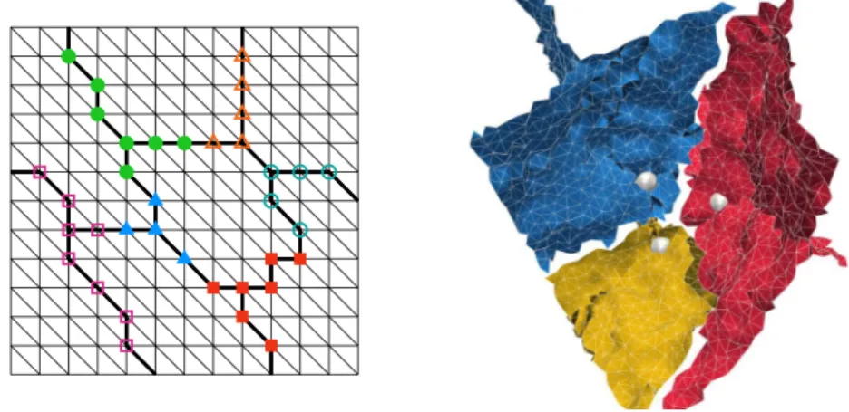
3

Fig. 2. Left: Partitioning of the RGDSW interface components into the respective parts of vertices and edges as required for the right hand side of the generalized eigenvalue problem in the RAGDSW method. Each component is partitioned into 5 subcomponents (4 edges, 1 vertex).

Right: The image shows a case, in which a NEC can consist of two disjoint connected components.

The interface of the domainΩ =∪³_i=1Ωiis indicated by thick black lines.

The reduced dimension GDSW coarse space is then defined completely analo-

260

gously to the GDSW coarse space. Thus the restriction of the null space elements

261

to the interface components is first extended by zero to the rest of the interface

262

nodes and then extended with minimal energy to the subdomain interiors to obtain

263

the coarse functions; see Figure 1 (bottom-right) for one of the coarse functions for

264

a two-dimensional diffusion problem.

265

We note that our RGDSW coarse space differs from those of [9] but that can

266

be regarded as a variant of the coarse spaces introduced in that paper.

267

7. The reduced dimension adaptive GDSW coarse space. For the re-

268

duced adaptive GDSW coarse space, we need to partition each interface component

269

ξ , as those of the previous section, into subcomponents. For a structured mesh and

270

domain decomposition, as in that section, we partition each ξ into subsets related to

271

the subdomain vertices, edges, and faces. With V , E , and F the sets of subdomain

272

vertices, edges, and faces, respectively, we define subcomponents ξ

i

of ξ such that

273

(7.1) {ξ

i

}

ⁿ_i=1^ξ

= {ξ ∩ c : c ∈ V ∪ E ∪ F ∧ c ∩ ξ 6= ∅},

274

where n

ξ

is the number of subcomponents of ξ ; see Figure 2 (left) for a two-

275

dimensional case. We next partition K

_ξξ^Ωξ

with respect to the subsets {ξ

_i

}

ⁿ_i=1^ξ

, into

276

K

_ξξ^Ωξ

= K

_ξ^Ωξ

iξ_j

ⁿξ

i,j=1 277

and, as before, we define the Schur complement by

278

S

ξξ

:= K

_ξξ^Ωξ

− K

_ξR^Ωξ

K

_RR^Ωξ

⁺

K

_Rξ^Ωξ

,

279

where K

_RR^Ωξ

+

is a pseudoinverse of K

_RR^Ωξ

; see Remark 9.1 and section 13. Fur-

280

thermore, let

281

(7.2) K e

ξξ

:= blockdiag

i=1,...,n_ξ

(K

_ξ^Ωξ

iξ_i

)

282

and introduce a generalized eigenvalue problem, given in matrix form by

283

S

ξξ

τ

∗,ξ

= λ

∗,ξ

K e

ξξ

τ

∗,ξ

.

284

As in section 5, the eigenvalues are sorted in a nondecreasing order and eigen-

285

vectors τ

∗,ξ

corresponding to λ

∗,ξ

≤ tol

ξ

are selected and then extended by zero to

286

Γ

^h

as τ

∗,Γ

. The coarse basis functions, i.e., the columns of Φ, corresponding to ξ

287

are the extensions v

∗,ξ

:= H

Γ

τ

∗,Γ

.

288

Remark 7.1. If tol

ξ

= 0 for all ξ ∈ P , the RAGDSW coarse space contains only

289

the coarse functions associated with the null space of the Schur complement S

ξξ

.

290

The latter is identical to the null space of K

^Ωξ

restricted to ξ . Thus, in this case,

291

RAGDSW reduces to RGDSW, and we have

292

V

RGDSW

= V

_RAGDSW⁰

⊂ V

_RAGDSW^tol(P)

.

293

8. Interface partitioning for RAGDSW on unstructured meshes. For

294

unstructured cases, we will define the partitioning P using nodal equivalence classes

295

and begin with definitions of connected components of finite element nodes and of

296

nodal equivalence classes. We note that equivalence classes have previously been

297

used in [9] for similar purposes.

298

Two finite element nodes x

^h₁

, x

^h₂

∈ Γ

^h

are said to be adjacent, if there exists

299

a finite element edge or face z ⊂ Γ such that x

^h₁

, x

^h₂

∈ z , the closure of z . A set

300

of nodes γ ⊂ Γ

^h

is said to form a connected component, if, for any two nodes

301

x

^h₀

, x

^h_s

∈ γ , there exists a path (x

^h₀

, . . . , x

^h_s

) , x

^h_i

∈ γ , of adjacent nodes.

302

For any node x

^h

∈ Ω , let

303

(8.1) n(x

^h

) := {i ∈ {1, 2, . . . , N} : x

^h

∈ Ω

i

}

304

be the set of indices of the subdomains which have x

^h

in common. To partition

305

a set of nodes γ ⊂ Γ

^h

, we define nodal equivalence classes (NECs) by the relation

306

x

^h₁

∼ x

^h₂

⇔ n(x

^h₁

) = n(x

^h₂

) , for any two nodes x

^h₁

, x

^h₂

∈ γ . We further partition each

307

NEC into its connected components based on the adjacency of nodes; cf. Figure 2

308

(right).

309

By N (x

^h

), we denote the NEC of a node x

^h

∈ γ , i.e., x

^h

∈ N (x

^h

) . If n(x

^h₂

) (

310

n(x

^h₁

) , then N (x

^h₁

) is said to be an ancestor of N (x

^h₂

) which in turn is a descendant

311

of N (x

^h₁

). If a NEC does not have an ancestor, we call it a root.

312

We note that for γ = Γ

^h

a root is a vertex (i.e., a coarse node) in the case

313

of cuboid subdomains. However, often for unstructured domain decompositions

314

obtained, e.g., by METIS [29], a root can be a coarse edge or coarse face as well; see

315

further the discussion in [9]. We note that for special cases of structured domain

316

decompositions, e.g., a beam built from a union of cubes, the same can occur.

317

We now give a general description of the interface partition for RAGDSW for

318

an unstructured mesh and domain decomposition. We will define components ξ ,

319

s.t. each ξ contains only one root and parts of its descendants. Furthermore, we

320

will assure that the resulting interface partition P is nonoverlapping to obtain a

321

partition P of connected disjoint components ξ ∈ P s.t.

322

Γ

^h

= [

ξ∈P 323

ξ.

Several specific constructions are possible. Relevant aspects are, e.g., obtaining

324

components of similar size, nondegenerate components, and parallel efficiency of

325

the construction.

326

For the results in this paper, we have constructed the interface partition in the

327

following way: We initialize each component ξ ∈ P with the nodes of a root and

328

add the remaining nodes in an iterative process.

329

Starting with the roots, we grow sets which will result in all the subsets ξ ∈ P .

330

In each step of an iteration, we add all nodes which are adjacent to elements of

331

each of the current sets, which have not been previously assigned, and which are

332

descendants of the root of the set. We repeat this process until all interface nodes

333

have been assigned to a ξ ∈ P . Figure 3 depicts sample partitions for two and three

334

dimensions.

335

We note that for the unstructured meshes in section 14, the average number of

336

degrees of freedom per eigenvalue problem is increased by roughly 50% and with

337

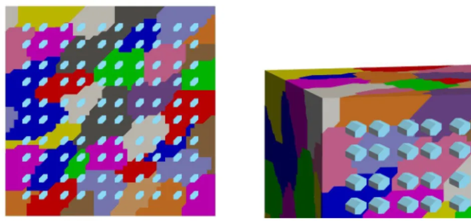
Fig. 3. Sample partitions in two dimensions (left) and three dimensions (right) for un- structured domain decompositions. For the two-dimensional case, the interface is given by thick black lines and the interface componentsξ∈ P by different markers. For the three-dimensional case, coarse nodes are indicated by white spheres; interface components are shown in different colors. For a clearer visualization, only those finite element faces are shown, whose nodes are all contained in the respective interface component. Thus, gaps indicate finite element faces, whose nodes are part of several interface components.

the maximum roughly doubled, compared to the face eigenvalue problems used in

338

the standard AGDSW.

339

As before, we partition each interface component into its subcomponents. Let

340

N

_Γh

be the set of NECs of Γ

^h

and for ξ ∈ P let

341

N

ξ

:= {ξ ∩ c : c ∈ N

Γ^h

∧ ξ ∩ c 6= ∅}.

342

Let n

ξ

:= |N

ξ

| be the number of NECs of ξ and let ξ

i

, i = 1, . . . , n

ξ

, be the

343

resulting decomposition of ξ into {ξ

i

}

ⁿ_i=1^ξ

= N

ξ

. We then have ξ

i

∩ ξ

j

= ∅ (i 6= j)

344

and ξ = S

nξ

i=1

ξ

i

.

345

Remark 8.1. If our problem satisfies a Neumann boundary condition on ∂Ω

N

⊂

346

∂Ω, in addition to a nonempty set ∂Ω

D

= ∂Ω \ ∂Ω

N

with a Dirichlet boundary

347

condition, then the construction of the RAGDSW coarse space and the proof of the

348

condition number estimate in sections 10 and 11 will essentially be the same. The

349

finite element nodes that lie on the Neumann boundary but not on the interface

350

Γ = S

i6=j

(∂Ω

i

∩ ∂Ω

j

) \ ∂Ω

D

are treated as interior nodes.

351

In the next section, we will first describe the adaptive GDSW coarse spaces in

352

variational form. Thereafter, we will derive a condition number estimate for the

353

preconditioned two-level additive Schwarz operator based on the coarse space in-

354

troduced above. We note that the proof remains valid for quite general interface

355

partitions P and is not restriced to the one of RAGDSW.

356

9. Variational description of adaptive GDSW-type coarse spaces. For

357

ξ ∈ P the index set n

^ξ

contains the indices of all adjacent subdomains, i.e., the

358

union of the index sets of all nodes x

^h

∈ ξ,

359

(9.1) n

^ξ

= [

x^h∈ξ

n(x

^h

).

360

As in section 5, Ω

ξ

is the closure of the union of adjacent subdomains, i.e., Ω

ξ

=

361

S

i∈n^ξ

Ω

i

.

362

Let G ⊂ Ω be any union of sets s ∈ {T

i

∩ T

j

6= ∅ : T

i

, T

j

∈ τ

h

}. By z

ξ G

(·), we

363

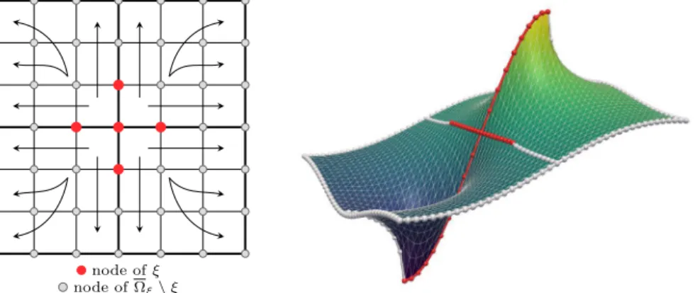
node ofξ node ofΩξ\ξ

Fig. 4. Graphical representation in two dimensions of the energy-minimal extension (9.3) fromξ∈ P toΩ_ξ (left) and sample energy-minimal extension for the diffusion equation (right) in which the RAGDSW interface componentξis highlighted in red and the remaining interface nodes in light gray.

denote an extension-by-zero operator from ξ ⊂ G to G:

364

(9.2)

z

ξ G

: X

^h

(ξ) →

w|

_G

: w ∈ V

^h

(Ω), w = 0 in Ω \ ξ v 7→ z

_{ξ G}

(v) :=

v(x

^h

) ∀x

^h

∈ ξ, 0 ∀x

^h

∈ G \ ξ.

365

Here, X

^h

(ξ) := {v : ξ → R

³

}.

366

By H

ξ Ω_ξ

(·), we denote a possibly nonunique (cf. Remark 9.1) energy-minimal

367

extension w.r.t. a

Ω_ξ

(·, ·) from ξ to Ω

ξ

: let V

_0,ξ^h

(Ω

ξ

) := {w|

Ω_ξ

: w ∈ V

^h

(Ω), w(x

^h

) =

368

0 ∀x

^h

∈ ξ} , then for τ

ξ

∈ X

^h

(ξ) , an extension v

ξ

:= H

ξ Ω_ξ

(τ

ξ

) ∈ V

^h

(Ω

ξ

) is given

369

by a solution of

370

(9.3) a

_Ωξ

(v

_ξ

, v) = 0 ∀v ∈ V

_0,ξ^h

(Ω

_ξ

), v

ξ

(x

^h

) = τ

ξ

(x

^h

) ∀x

^h

∈ ξ;

371

cf. Figure 4. We note that the extension is computed with a homogeneous Neumann

372

boundary condition on ∂Ω

_ξ

.

373

As in section 8, let {ξ

i

}

ⁿ_i=1^ξ

be the set of all NECs of a ξ ∈ P . Then ξ

_i

∩ ξ

_j

= ∅

374

( i 6= j ) and ξ = S

ⁿξ

i=1

ξ

_i

holds. We define the symmetric, positive definite bilinear

375

form

376

(9.4) c

ξ

(u, v) :=

nξ

X

i=1

c

ξ_i

(u, v) ∀u, v ∈ X

^h

(ξ),

377

with

378

(9.5) c

ξ_i

(u, v) := a

Ω_ξi

z

ξ_i Ω_ξi

(u), z

ξ_i Ω_ξi

(v)

∀u, v ∈ X

^h

(ξ).

379

The corresponding norm is defined by

380

(9.6) kuk

²_cξ

:= c

_ξ

(u, u) ∀u ∈ X

^h

(ξ).

381

We define the following generalized eigenvalue problem on ξ ∈ P : Find τ

_∗,ξ

∈ X

^h

(ξ)

382

such that

383

a

_Ωξ

H

_{ξ Ωξ}

(τ

_∗,ξ

), H

_{ξ Ωξ}

(θ)

= λ

_∗,ξ

c

_ξ

(τ

_∗,ξ

, θ) ∀θ ∈ X

^h

(ξ) . (9.7)

384385

The eigenvalues are again sorted in nondescending order; i.e., λ

1,ξ

≤ λ

2,ξ

≤ ... ≤

386

λ

m,ξ

and the eigenmodes accordingly, where m = dim X

^h

(ξ) . Furthermore, let

387

the eigenmodes τ

_∗,ξ

satisfy c

ξ

(τ

k,ξ

, τ

j,ξ

) = δ

kj

, where δ

kj

is the Kronecker delta

388

symbol. We select all eigenmodes τ

_∗,ξ

where the eigenvalues are below a certain

389

threshold, i.e., λ

_∗,ξ

≤ tol

ξ

. Then, the coarse basis functions corresponding to ξ are

390

the extensions

391

(9.8) v

_∗,ξ

:= H

Γ Ω

τ

_Γ

∈ V

₀^h

(Ω), τ

_Γ

:= z

_{ξ Γ}

(τ

_∗,ξ

),

392

of the selected τ

_∗,ξ

, where v

_∗,ξ

= H

Γ Ω

(τ

Γ

) is given by the solution v

_∗,ξ

∈ V

₀^h

(Ω)

393

that satisfies

394

(9.9) a

Ω_l

(v

_∗,ξ

, w) = 0 ∀w ∈ V

₀^h

(Ω

l

) , l = 1, ..., N, v

∗,ξ

(x

^h

) = τ

Γ

(x

^h

) ∀x

^h

∈ Γ

^h

.

395

We note that, contrary to (9.7), v

_∗,ξ

vanishes on ∂Ω

_ξ

since τ

_Γ

= z

_{ξ Γ}

(τ

_∗,ξ

) and since

396

v

_∗,ξ

= H

_{Γ Ω}

τ

_Γ

∈ V

₀^h

(Ω) . Therefore, (9.9) has a unique solution.

397

For a general interface partition P , we define the adaptive GDSW coarse space

398

as

399

(9.10) V

_P

:= M

ξ∈P

span {v

k,ξ

: λ

k,ξ

≤ tol

ξ

} .

400

The standard AGDSW coarse space (see [21]) is based on the partition

401

P := F ∪ E ∪ V.

402

Since vertices, edges, and faces are NECs, we then have

403

c

ξ

(u, v) = a

Ω_ξ

z

ξ Ω_ξ

(u), z

ξ Ω_ξ

(v)

404

if ξ is a vertex, an edge, or a face.

405

Remark 9.1. For the diffusion case the energy-minimal extension defined by

406

(9.3) has a unique solution. If an interface component ξ is a straight edge or a vertex

407

then 1 or 3 rotations, respectively, are in the null space of the extension operator

408

for linear elasticity. However, as all solutions of (9.3) have the same energy, the

409

choice of the particular solution does not influence the solution of the generalized

410

eigenvalue problem (9.7): let v

_∗,ξ

= H

ξ Ωξ

(τ

_∗,ξ

) be a solution of (9.3). Then all

411

solutions are given by v

_∗,ξ

+ r , where r ∈ range H

ξ Ω_ξ

(0)

; for linear elasticity r

412

is a rigid body mode. Since r ∈ V

_0,ξ^h

(Ω

_ξ

) , we have a

_Ωξ

r, H

_{ξ Ωξ}

(θ)

= 0 by the

413

definition of H

_{ξ Ωξ}

(θ) . Therefore, v

_∗,ξ

+ r solves (9.3) and

414

a

_Ωξ

v

_∗,ξ

+ r, H

_{ξ Ωξ}

(θ)

= a

_Ωξ

v

_∗,ξ

, H

_{ξ Ωξ}

(θ)

∀θ ∈ X

^h

(ξ) .

415

As a consequence, any operator defined by (9.3) yields the same generalized eigen-

416

value problem (9.7). In section 13, we will provide some remarks on how to find

417

the solution of (9.3) when it is not unique.

418

Remark 9.2. We note that the left hand side of eigenvalue problem (9.7) is

419

singular and its kernel contains the constant functions for the scalar diffusion case

420

and the rigid body modes for linear elasticity. Therefore, the null space has a

421

dimension of 1 for the scalar diffusion problem and at least 3 for linear elasticity.

422

For a vertex (i.e., ξ = v ∈ V) the problem has only one (scalar diffusion) and three

423

(linear elasticity) degrees of freedom. Thus, in the latter case, the solution is given

424

by the vertex basis functions of the GDSW coarse space, i.e., the three translations

425

in case of linear elasticity; cf. [21] and [7].

426

10. Spectral projections. We will now consider the projections

427

Π

P

w := X

ξ∈P

Π

ξ

w, Π

ξ

w := X

λk,ξ≤tolξ

c

ξ

(w, v

k,ξ

)v

k,ξ

(10.1)

428 429

onto the space V

_P

. Here, v

k,ξ

are the energy-minimal extensions of the eigenfunc-

430

tions determined by (9.8) and λ

k,ξ

the corresponding eigenvalues from (9.7). For

431

ξ ∈ P , let d

ξ

: X

^h

(ξ) × X

^h

(ξ) → R be the symmetric, positive semidefinite bilinear

432

form

433

d

_ξ

(·, ·) := a

_Ωξ

(H

ξ Ωξ

(·), H

ξ Ωξ

(·)).

(10.2)

434435

For any union B ⊂ Ω of finite elements T ∈ τ

_h

, let

436

|v|

_a(B)

:= p

a

B

(v, v) ∀v ∈ V

^h

(Ω).

(10.3)

437438

We find that

439

(10.4) |v|

²_dξ

:= d

_ξ

(v, v) =

H

ξ Ωξ

(v)

2

a(Ωξ)

≤ |v|

²_a(Ω

ξ)

∀ v ∈ V

^h

(Ω),

440

due to the energy-minimal property of the extension operator.

441

Using standard arguments of spectral teory, we obtain two important properties

442

of the projection Π

ξ

, required for the proof of the condition number estimate in

443

section 11; cf., e.g., [21, Lemma 5.3] and [20, Lemma 4.1].

444

Lemma 10.1. Let the eigenpairs {(τ

k,ξ

, λ

k,ξ

)}

^dim

X^h(ξ)

k=1

from (9.7) be chosen

445

such that c

ξ

(τ

k,ξ

, τ

j,ξ

) = δ

kj

and such that the eigenpairs are sorted in nondescending

446

order w.r.t. the eigenvalues. Then the operator Π

ξ

defines a projection which is

447

orthogonal with respect to the bilinear form d

ξ

(·, ·) and therefore

448

|u|

²_d

ξ

= |Π

ξ

u|

²_d

ξ

+ |u − Π

_ξ

u|

²_d

ξ

, ∀u ∈ X

^h

(ξ).

449

In addition, we have, from spectral theory,

450

ku − Π

_ξ

uk

²_c

ξ

≤ 1

tol

ξ

|u − Π

_ξ

u|

²_d

ξ

.

451452

The following lemma follows directly from Lemma 10.1; cf. [21, Lemma 2].

453

Lemma 10.2. For ξ ∈ P and u ∈ V

^h

(Ω) it holds that

454

ku − Π

ξ

uk

²_c

ξ

≤ 1

tol

ξ

X

k∈n^ξ

|u|

²_a(Ω

k)

.

455

Proof. We have

456

ku − Π

_ξ

uk

²_c

ξ

Lemma10.1

≤ 1

tol

ξ

|u − Π

_ξ

u|

²_d

ξ

≤ 1

tol

ξ

|u|

²_d

457 ξ

(10.4)

≤ 1

tol

_ξ

|u|

²_a(Ω

ξ)

= 1 tol

_ξ

X

k∈n^ξ

|u|

²_a(Ω

k)

.

458 459

11. Convergence analysis. To prove a condition number estimate, we will

460

prove the existence of a stable decomposition; cf. [43, Chapter 2]. We therefore

461

define the coarse interpolation I

0

:= Π

_P

as the projection onto the coarse space

462

V

0

:= V

_P

; cf. (9.10) and (10.1). Thus the coarse component of the stable decompo-

463

sition is defined as

464

u

0

:= I

0

u := Π

P

u.

465466 467

Lemma 11.1. For ξ ∈ P and u ∈ V

^h

(Ω), we have

468

ku − u

0

k

²_cξ

= c

ξ

(u − u

0

, u − u

0

) ≤ 1 tol

ξ

X

k∈n^ξ

|u|

²_a(Ω

k)

.

469

Proof. We have

470

ku − u

₀

k

²_cξ

=

n_ξ

X

i=1

|z

ξi Ω_ξi

(u − Π

_P

u)|

²_a(Ω

ξi) 471

=

nξ

X

i=1

|z

ξ_i Ω_ξi

(u − Π

ξ

u)|

²_a(Ω

ξi) 472

= ku − Π

ξ

uk

²_cξ

473

Lemma10.2

≤ 1

tol

ξ

X

k∈n^ξ

|u|

²_a(Ω

k)

.

474

475

Next, we derive an estimate for the energy of the coarse component.

476

Lemma 11.2. It holds that

477

|u

₀

|

²_a(Ω)

≤ 2 |u|

²_a(Ω)

+ 2C

τ

tol

_P

X

ξ∈P

X

k∈n^ξ

|u|

²_a(Ω

k)

≤ 2

1 + C

τ

N

^ξ

tol

_P

|u|

²_a(Ω)

,

478 479

where C

τ

is the maximum number of vertices of any element T ∈ τ

h

(Ω) , and

480

(11.1) N

^ξ

:= max

1≤i≤N

|P(Ω

i

)|, P (Ω

i

) := {ξ ∈ P : ξ ∩ Ω

i

6= ∅}

481

is the maximum number of interface components ξ ∈ P of any subdomain, and

482

tol

P

:= min

ξ∈P

tol

ξ

.

483

Proof. We can use the fact that u

₀

is energy-minimal w.r.t. |·|

_a,Ω

i

for each

484

subdomain Ω

_i

, i.e., u

₀

= H

Γ Ω

(u

₀

) , and obtain

485

|u

0

|

²_a(Ω)

≤ 2|H

Γ Ω

(u)|

²_a(Ω)

+ 2|H

Γ Ω

(u − u

0

)|

²_a(Ω)

486

≤ 2|u|

²_a(Ω)

+ 2|z

Γ Ω

(u − u

0

)|

²_a(Ω)

.

487488

Let

489

(11.2) N

_ec,P

:= [

ξ∈P

{ξ

i

, i = 1, . . . , n

ξ

}

490

be the set of interface components of the ξ ∈ P partitioned into their nodal equiv-

491

alence classes ξ

_i

, i = 1, . . . , n

_ξ

. Then, ξ

_i

∩ ξ

_j

= ∅ for i 6= j , and S

ξi∈Nec,P

ξ

_i

= Γ

^h

,

492

and

493

|z

Γ Ω

(u − u

0

)|

²_a(Ω)

= | X

ξi∈Nec,P

z

ξ_i Ω

(u − u

0

)|

²_a(Ω)

494

= X

T∈τh(Ω)

| X

ξ_i∈Nec,P

z

ξ_i Ω

(u − u

0

)|

²_a(T)

.

495 496

There can be at most C

τ

NECs ξ

i

that are nonzero in any element T . Thus, we

497

have using the Cauchy–Schwarz inequality

498

X

T∈τh(Ω)

| X

ξ_i∈Nec,P

z

_{ξi Ω}

(u − u

₀

)|

²_a(T)

≤ X

T∈τh(Ω)

C

_τ

X

ξ_i∈Nec,P

|z

_{ξi Ω}

(u − u

₀

)|

²_a(T)

499

= C

_τ

X

ξi∈Nec,P

|z

ξi Ω

(u − u

₀

)|

²_a(Ω

ξi) 500

= C

τ

X

ξ∈P

ku − u

0

k

²_cξ

501

≤ C

_τ

tol

P

X

ξ∈P

X

k∈n^ξ

|u|

²_a(Ωk)

,

502 503

where in the last step we have used Lemma 11.1. Thus,

504

|u

0

|

²_a(Ω)

≤ 2|u|

²_a(Ω)

+ 2 C

τ

tol

_P

X

ξ∈P

X

k∈n^ξ

|u|

²_a(Ωk)

≤ 2

1 + C

τ

N

^ξ

tol

_P

|u|

²_a(Ω)

.

505

506

In Theorem 11.4, we will derive estimates based on the product of u − u

0 507

and a partition of unity function θ

i

associated with each subdomain. We employ an

508

overlapping decomposition { Ω ˜

i

}

^N_i=1

with overlap h by extending the nonoverlapping

509

decomposition {Ω

i

}

^N_i=1

by one layer of finite elements. The estimates are carried

510

out separately on Ω ˜

_i

\ Ω

_i

and Ω

_i

: the former locally and the latter globally. The

511

following lemma covers both cases.

512

Lemma 11.3. Let l ∈ {0, 1, . . . , N } and B = ˜ Ω

_l

\ Ω

_l

, if l > 0 , and B = Ω

₀

:= Ω

513

for l = 0 . Furthermore, let Ψ : B → R s.t. Ψ|

ξi

is constant on ξ

_i

∈ N

ec,P

, ξ

_i

⊂ B ,

514

i.e., Ψ(x

^h

) = C

_i

for all x

^h

∈ ξ

_i

. Additionally, we assume that 0 ≤ Ψ ≤ 1 and

515

Ψ(x

^h

) = 0 for x

^h

∈ / Γ

^h

∩ B . Then,

516

I

^h

(Ψ · (u − u

0

))

2

a(B)

≤ C

τ

tol

_P

X

ξ∈P(Ωl)

X

k∈n^ξ

|u|

²_a(Ω

k)

,

517

where I

^h

(·) is the pointwise interpolation operator of the finite element space V

^h

(Ω).

518

Proof. We define the set N

_ec,P

(Ω

l

) := {ξ

j

∈ N

_ec,P

: ξ

j

∩ Ω

l

6= ∅} of NECs that

519

are part of or touch Ω

l

. Given that P (Ω

0

) = P , it is N

_ec,P

(Ω

0

) = N

_ec,P

. Since

520

z

ξ_i B

(·) acts as an identity operator on ξ

i

, we have

521

I

^h

(Ψ · (u − u

0

))

2 a(B)

=

X

ξ_i∈Nec,P(Ω_l)

z

ξi B

(Ψ · (u − u

0

))

2 a(B) 522

= X

T∈τh(B)

X

ξ_i∈Nec,P(Ω_l)

z

ξ_i B

(Ψ · (u − u

0

))

2 a(T)

.

523 524

There can be at most C

τ

NECs ξ

i

that are nonzero in any element T . Thus, we

525

have using the Cauchy–Schwarz inequality

526

X

ξi∈Nec,P(Ω_l)

z

_{ξi B}

(Ψ · (u − u

₀

))

2 a(T)

≤ C

_τ

X

ξi∈Nec,P(Ω_l)

z

_{ξi B}

(Ψ · (u − u

₀

))

2 a(T) 527

528

and consequently

529

I

^h

(Ψ · (u − u

0

))

2

a(B)

≤ C

τ

X

ξ_i∈Nec,P(Ω_l)

z

ξi Ω_ξi

(Ψ · (u − u

0

))

2 a(Ω_ξi)

.

530 531