Technical Report Series Center for Data and Simulation Science

Technical Report Series

Center for Data and Simulation Science

Alexander Heinlein, Axel Klawonn, Martin Lanser, Janine Weber

A Frugal FETI-DP and BDDC Coarse Space for Heterogeneous Problems

Technical Report ID: CDS-2019-18

Available at https://kups.ub.uni-koeln.de/id/eprint/10363

Submitted on December 1, 2019

HETEROGENEOUS PROBLEMS

ALEXANDER HEINLEIN

, AXEL KLAWONN

, MARTIN LANSER

, AND JANINE WEBER

December 2, 2019

Abstract. The convergence rate of domain decomposition methods is generally determined by the eigenvalues of the preconditioned system. For second-order elliptic partial differential equations, coefficient discontinuities with a large contrast can lead to a deterioration of the convergence rate.

Only by implementing an appropriate coarse space or second level, a robust domain decomposition method can be obtained. In this article, a new frugal coarse space for FETI-DP (Finite Element Tearing and Interconnecting - Dual Primal) and BDDC (Balancing Domain Decomposition by Con- straints) methods is presented, which has a lower set-up cost than competing adaptive coarse spaces.

In particular, in contrast to adaptive coarse spaces, it does not require the solution of any local generalized eigenvalue problems. The approach considered here aims at a low-dimensional approxi- mation of the adaptive coarse space by using appropriate weighted averages and is robust for a broad range of coefficient distributions for diffusion and elasticity problems. In this article, the robustness is heuristically justified as well as numerically shown for several coefficient distributions. The new coarse space is compared to adaptive coarse spaces, and parallel scalability up to 262 144 parallel cores for a parallel BDDC implementation with the new coarse space is shown. The superiority of the new coarse space over classic coarse spaces with respect to parallel weak scalability and time to solution is confirmed by numerical experiments.

Key words. FETI-DP, BDDC, robust coarse spaces, adaptive domain decomposition methods AMS subject classifications.

1. Introduction. Domain decomposition methods are robust and parallel scal- able iterative solvers for large systems of equations arising from the discretization of partial differential equations, e.g., by finite elements. In general, the computa- tional domain is decomposed into a number of overlapping or nonoverlapping sub- domains. Here, we focus on two classes of nonoverlapping domain decomposition methods, namely FETI-DP (Finite Element Tearing and Interconnecting - Dual Pri- mal) [13, 14,42, 43] and BDDC (Balancing Domain Decomposition by Constraints) [8, 9, 45, 47,48] methods. Both algorithms have successfully been applied to a wide range of model problems and have been shown to be parallel scalable for up to hundreds of thousands of compute cores [1, 2, 30–33, 39, 61]. In general, domain decomposition methods obtain their robustness and parallel scalability from an appropriate coarse space, i.e., a second level. For nonoverlapping domain decomposition methods, such a coarse space can be constructed by simply sub-assembling the system in selected pri- mal variables using geometric information. For these classic coarse spaces, condition number bounds have been proven for a wide range of model problems [38, 41–43, 51].

However, the respective condition number bounds are only valid under certain restric- tive assumptions on the coefficient functions of the differential equation considered, e.g., the diffusion coefficient in case of a diffusion problem or the Young modulus in case of a linear elasticity problem.

∗

This work was supported in part by Deutsche Forschungsgemeinschaft (DFG) through the Pri- ority Programme 1648 "Software for Exascale Computing" (SPPEXA) under grant KL 2094/4-2.

†

Department of Mathematics and Computer Science, University of Cologne, Weyer- tal 86-90, 50931 Köln, Germany, alexander.heinlein@uni-koeln.de, axel.klawonn@uni-koeln.de, martin.lanser@uni-koeln.de, janine.weber@uni-koeln.de, url: http://www.numerik.uni-koeln.de

‡

Center for Data and Simulation Science, University of Cologne, Germany, url: http://www.cds.

uni-koeln.de

1

For more general and complex coefficient functions with arbitrary jumps along or across the interface, the classic condition number bounds do not hold anymore and the convergence rate of the classic domain decomposition methods typically deteriorates.

Thus, different adaptive coarse space techniques for several domain decomposition methods have been developed within recent years to cope with heterogeneous coeffi- cient functions with large jumps; see, e.g., [3, 5,7, 11, 12, 15–17,19–21, 26–29, 35, 36,49, 50, 52, 53, 55, 56]. Most of these methods rely on the solution of certain local general- ized eigenvalue problems and use selected eigenvectors to enhance the coarse space.

By including these adaptive coarse spaces, the algorithm is again robust with respect to discontinuous coefficient functions for both diffusion and elasticity problems. In particular, contrast independent condition number estimates can be proven for most of those adaptive coarse spaces. As a drawback in a parallel implementation, the set- up and the solution of the eigenvalue problems take up a significant amount of time.

In [23], we introduced the concept of training a neural network to make an automatic decision on which parts of the interface for two dimensional model problems, i.e., on which edges, the solution of the eigenvalue problem is indeed necessary to obtain a robust algorithm. This can reduce the time to solution significantly.

A further important experimental observation is that for many realistic coeffi- cient distributions often only a small number of jumps with respect to a specific edge or face occurs for a large number of edges and faces. Thus, for many edges and faces, the computation of all eigenvectors is indeed unnecessary since already a sin- gle or a small number of constraints is sufficient for robustness on these edges and faces. In the present paper, we introduce an alternative and more frugal approach. In principle, we aim to compute a low-dimensional approximation of the adaptive coarse space by constructing weighted averages along edges or faces. Earlier works [18,20,44]

showed that heuristic coarse spaces, which approximate adaptive coarse spaces and do not require the solution of local generalized eigenvalue problems, can be constructed for overlapping Schwarz domain decomposition methods. Here, using our experience with adaptive coarse spaces, we construct constraints in a similar approach. We will observe that for many realistic coefficient distributions the resulting constraints are already sufficient for fast convergence. The approach presented here can further be in- terpreted as a generalization of the classic weighted averages over edges as introduced in [38]. In fact, for the case of discontinuities which are aligned with the interface, our new constraints enforce comparable constraints as those classic weighted averages.

However, our new weighted constraints additionally lead to robust algorithms in more general and complex cases of discontinuities not aligned with the interface. In gen- eral, for completely arbitrary coefficient jumps additional constraints, i.e., obtained by adaptive coarse spaces, can be necessary to further improve the convergence of the algorithm.

To provide a brief impression on the capability of our proposed coarse space, we

consider a simple exemplary coefficient distribution with coefficient jumps as in Fig-

ure 3 (left). We compare numerical results for so-called standard approaches, i.e., the

classic weighted edge averages [38], an adaptive coarse space variant [49, 50], and our

proposed frugal coarse space in Table 1. While our approach is competitive to the

adaptive approach, the one with classic weighted edge averages clearly fails to provide

a robust algorithms, although the dimension of the classic coarse space is three times

larger. Notably, in contrast to the adaptive constraints, the construction of our new

constraints is easily parallelizable and fairly cheap, i.e., the resulting coarse space can

be computed with less effort than a few CG (conjugate gradient) iterations since it

does not require the solution of any eigenvalue problems. Thus, our new approach

adaptive classic weighted avg. new approach

H/h # c. cond it # c. cond it # c. cond it

stationary diffusion

8 4 3.60 12 12 61 559.3 20 4 3.60 12

16 4 3.95 13 12 99 656.1 24 4 3.96 13

32 4 5.02 15 12 1.1775e05 26 4 5.04 15

Table 1

Dimensions of the coarse space (# c.), condition numbers (cond) and iteration numbers (it) for the FETI-DP algorithm for a stationary diffusion problem on the unit square with 4 × 4 subdomains for the coefficient distribution as in Figure 3 (left). Homogeneous Dirichlet boundary conditions on the left side of the unit square. The higher coefficient is 1e6 and the lower coefficient is 1.

could be implemented as a default rule to enhance the coarse space when no im- plementation of adaptive coarse space techniques is available or the time to solution should be reduced. Our numerical experiments show that our new frugal approach leads to a robust algorithm for problems with a realistic coefficient distribution and can especially outperform classic edge and face averages in cases of complex coefficient functions.

The remainder of the paper is organized as follows. In section 2, we first introduce the model problems and the necessary notation to outline our domain decomposition methods. We then describe both the FETI-DP and the BDDC algorithm in more detail. In section 3, we give a detailed description of our new constraints. For the convenience of the reader, we first explain the construction for diffusion problems, which is the simpler case. For the case of linear elasticity, we then give the corre- sponding formulae based on weighted rigid body modes. We provide first serial results by applying the proposed approach to different coefficient distributions, proving that our algorithm is robust, in section 4. Finally, in section 5, we present results com- paring our new approach to classic averages using our parallel BDDC implementation applied to difficult model problems. For all our numerical tests, we consider stationary linear diffusion and linear elasticity problems.

2. Algorithms and model problems. As a model problem, we consider both stationary linear diffusion problems as well as linear elasticity problems in two and three dimensions. We will focus on highly heterogeneous problems with large dis- continuities in the material stiffness or the diffusion coefficient, respectively. For the remainder of this section, we denote by d = 2, 3 the dimension of our domain Ω ⊂ R ^d . 2.1. Stationary diffusion. As a first model problem, we consider a stationary diffusion problem in its variational form with various coefficient functions ρ : Ω → R , which may have large jumps. We assume that one part of the boundary of the domain,

∂Ω _D , has homogeneous Dirichlet boundary conditions, while ∂Ω _N := ∂Ω \ ∂Ω _D has a natural boundary condition ^∂u _∂x = g. Throughout this paper, we only consider a homogeneous flow g = 0. Thus, the model problem can be written as: Find u ∈ H ₀ ¹ (Ω, ∂Ω D ):= {u ∈ H ¹ (Ω) : u = 0 on ∂Ω D }

(2.1)

Z

Ω

ρ∇u · ∇v dx = Z

Ω

f v dx ∀v ∈ H ₀ ¹ (Ω, ∂Ω D ).

The concrete examples of different coefficient functions ρ as well as the concrete choice

of the boundary conditions are given in detail in section 4.

2.2. Linear Elasticity. We consider an elastic body Ω ⊂ R ^d , d = 2, 3. We denote by u : Ω → R ^d the displacement of the body, by f a given volume force, and by g a given surface force onto the body, respectively. Here, we only consider a homogeneous surface force g = 0.

We introduce the vector-valued Sobolev space H ¹ ₀ (Ω, ∂Ω D ) := (H ₀ ¹ (Ω, ∂Ω D )) ^d . The problem of linear elasticity consists in finding the displacement u ∈ H ¹ ₀ (Ω, ∂Ω D ), such that

(2.2)

Z

Ω

G ε(u) : ε(v) dx + Z

Ω

Gβ divu divv dx = hF, vi

for all v ∈ H ¹ ₀ (Ω, ∂Ω D ) for given material functions G : Ω → R and β : Ω → R and the right-hand side

hF, vi = Z

Ω

f ^T v dx.

The material parameters G and β depend on the Young modulus E > 0 and the Poisson ratio ν ∈ (0, 1/2) given by G = E/(1 + ν) and β = ν/(1 − 2ν ). Here, we restrict ourselves to compressible linear elasticity; hence the Poisson ratio ν is bounded away from 1/2. Furthermore, the linearized strain tensor ε = (ε ij ) ij is defined by ε _ij (u) := ¹ ₂ ( ^∂u _∂x

j

+ ^∂u _∂x

i

) and we introduce the notation ε(u) : ε(v) :=

d

X

i,j=1

ε _ij (u)ε _ij (v), (ε(u), ε(v)) _L

_(Ω) :=

Z

Ω

ε(u) : ε(v) dx.

The corresponding bilinear form associated with linear elasticity can now be writ- ten as

a(u, v) = (G ε(u), ε(v)) _L

_(Ω) + (Gβ div u, div v) _L

_(Ω) .

Since we will only consider compressible elastic materials, it is sufficient to discretize our elliptic problem by low order conforming finite elements, e.g., linear or trilinear elements.

2.3. The FETI-DP and the BDDC algorithm.

2.3.1. Domain Decomposition. Let us briefly describe the preliminaries for our domain decomposition methods to introduce the FETI-DP and BDDC algorithms.

For a given domain Ω ⊂ R ^d , d = 2, 3, we assume a decomposition into N ∈ N nonover- lapping subdomains Ω _i , i = 1, . . . , N , such that Ω = S N

i=1 Ω _i . We presume that each of the subdomains Ω _i is the union of finite elements such that we have matching finite element nodes on the interface Γ :=

S N i=1 ∂Ω i

\ ∂Ω. In our case, each subdomain is the union of shape regular elements of diameter O(h). The diameter of a subdomain Ω _i is denoted by H _i or, generically, by H= max _i (H _i ). We denote by W _i the local finite element space associated with Ω _i . In case of a two-dimensional domain Ω ⊂ R ² , the finite element nodes on the interface are either vertex nodes, belonging to the boundary of more than two subdomains, or edge nodes, belonging to the boundary of exactly two subdomains. For the case of a three-dimensional domain Ω ⊂ R ³ , edge nodes also belong to the boundary of more than two subdomains, and the interface further consists of face nodes, belonging to the boundary of exactly two subdomains;

see, e.g., [37, Def. 2.1 and Def. 2.2] and [42, Def. 3.1]. All finite element nodes

inside a subdomain Ω i are denoted as interior nodes. For a given domain decompo- sition, we obtain local finite element problems K ⁽ⁱ⁾ u ⁽ⁱ⁾ = f ⁽ⁱ⁾ with K ⁽ⁱ⁾ : W i → W i

and f ⁽ⁱ⁾ ∈ W i by restricting the considered differential equation (see subsection 2.1 and subsection 2.2) to Ω i and discretizing its variational formulation in the finite ele- ment space W i . Let us remark that the matrices K ⁽ⁱ⁾ are, in general, not invertible for subdomains which have no contact to the Dirichlet boundary. We define the product space W := Q N

i=1 W i and denote by W c ⊂ W the space of functions in W that are continuous on Γ. For FETI-DP and BDDC, we partition the finite element variables u ⁽ⁱ⁾ ∈ W i into interior variables u ⁽ⁱ⁾ _I , and, on the interface, into dual variables u ⁽ⁱ⁾ _∆ and primal variables u ⁽ⁱ⁾ _Π . We denote the respective degrees of freedom by the indizes I, ∆ and Π. In the present article, we always choose all variables belonging to vertices as primal variables. Thus, the dual variables always belong to edges and/or faces.

Note that other choices are possible. Finally, we introduce the space f W , consist- ing of functions w ∈ W that are continuous in the primal variables. We thus have W c ⊂ W f ⊂ W .

2.3.2. Standard FETI-DP. As a first step for both the FETI-DP [13, 14] and the BDDC [9,47] algorithm, we compute the local stiffness matrices K ⁽ⁱ⁾ and the local right-hand sides f ⁽ⁱ⁾ for every subdomain Ω i , i = 1, . . . , N . The local problems are completely decoupled and, as already mentioned, the matrices K ⁽ⁱ⁾ are, in general, not invertible for subdomains without contact to the Dirichlet boundary. Both the FETI-DP and the BDDC algorithm deal with this difficulty by sub-assembling the decoupled system in selected primal variables Π.

Let us first introduce the simple restriction operators R i : V ^h → W i , i = 1, ..., N, the block vectors u ^T := u ^(1)T , ..., u ^(N)T

and f ^T := f ^(1)T , ..., f ^{(N )T}

, and the block matrices R ^T := R ^T ₁ , ..., R ^T _N

and K = diag K ⁽¹⁾ , ..., K ^{(N )}

. We then obtain the fully assembled system

(2.3) K g = R ^T KR

and the fully assembled right-hand side

(2.4) f g = R ^T f.

The block matrix K is not invertible as long as a single subdomain has no contact to the Dirichlet boundary. Thus, the system Ku = f has no unique solution, i.e., an unknown vector u might be discontinuous on the interface. Let us now describe how the continuity of u ∈ W := W 1 × ... × W N on the interface is enforced using FETI-DP. Here, we use a presentation of the FETI-DP method which is very similar to the compact notation in [36].

We assume the following partitioning of the local stiffness matrices K ⁽ⁱ⁾ , the local load vectors f ⁽ⁱ⁾ , and the local solutions u ⁽ⁱ⁾ using the subdivision of the degrees of freedom as introduced in subsection 2.3.1:

K ⁽ⁱ⁾ =







K _II ⁽ⁱ⁾ K _∆I ^(i)T K _ΠI ^(i)T K _∆I ⁽ⁱ⁾ K _∆∆ ⁽ⁱ⁾ K _Π∆ ^(i)T K _ΠI ⁽ⁱ⁾ K _Π∆ ⁽ⁱ⁾ K _ΠΠ ⁽ⁱ⁾





 , u ⁽ⁱ⁾ =





 u ⁽ⁱ⁾ _I u ⁽ⁱ⁾ _∆ u ⁽ⁱ⁾ _Π





 , and f ⁽ⁱ⁾ =





 f _I ⁽ⁱ⁾ f _∆ ⁽ⁱ⁾ f _Π ⁽ⁱ⁾





 .

It is often convenient to further introduce the union of interior and dual degrees

of freedom as an additional set of degrees of freedom denoted by the index B. This

leads to a more compact notation and we can define the following matrices and vectors

K _BB ⁽ⁱ⁾ =

"

K _II ⁽ⁱ⁾ K _∆I ^(i)T K _∆I ⁽ⁱ⁾ K _∆∆ ⁽ⁱ⁾

#

, K _ΠB ⁽ⁱ⁾ = h

K _ΠI ⁽ⁱ⁾ K _Π∆ ⁽ⁱ⁾

i , and f _B ⁽ⁱ⁾ = h

f _I ^(i)T f _∆ ^(i)T i ^T

. We then introduce the block diagonal matrices K BB = diag ^N _i=1 K _BB ⁽ⁱ⁾ , K II = diag ^N _i=1 K _II ⁽ⁱ⁾ , K ∆∆ = diag ^N _i=1 K _∆∆ ⁽ⁱ⁾ , and K ΠΠ = diag ^N _i=1 K _ΠΠ ⁽ⁱ⁾ . Analogously, we obtain the block vec- tor u B = [u ^(1)T _B , . . . , u ^(N _B ^)T ] ^T and the block right-hand side f B = h

f _B ^(1)T , . . . , f _B ^{(N )T} i T

. For the FETI-DP algorithm, continuity in the primal variables Π is enforced by a finite element assembly process, while continuity in the dual variables ∆ is en- forced iteratively by Lagrangian multipliers λ. To describe the primal assembly pro- cess, we introduce the assembly operators R ⁽ⁱ⁾ _Π

, which consist of values in {0, 1}.

This yields the primally assembled matrices K e ΠΠ = P N

i=1 R ^(i)T _Π K _ΠΠ ⁽ⁱ⁾ R _Π ⁽ⁱ⁾ , K e ΠB = h

R _Π ^(1)T K _ΠB ⁽¹⁾ , . . . , R ^(N _Π ^)T K _ΠB ^{(N )} i

, and right-hand side f e =

f _B ^T , P N

i=1 R ^(i)T _Π f _Π ^{(i) T T} . In order to enforce continuity in the dual degrees of freedom, we introduce a jump operator B B = [B ⁽¹⁾ _B . . . B _B ^(N) ] with B _B ⁽ⁱ⁾ having zero entries for the interior degrees of freedom and entries out of {−1, 1} for the dual degrees of freedom. The entries for the dual degrees of freedom are chosen such that B B u B = 0 if and only if u B is continuous on the interface. This continuity condition is enforced by the Lagrange multipliers λ, which act between two degrees of freedom each.

The FETI-DP master system is then given by (2.5)





K _BB K e _ΠB ^T B _B ^T K e _ΠB K e _ΠΠ O

B _B O O







 u _B

˜ u _Π

λ



 =



 f B

f ˜ Π

0



 .

To solve (2.5), the variables u _B and u ˜ _Π are eliminated, resulting in a linear system for the Lagrange multipliers λ. By block Gaussian elimination, we thus obtain the standard FETI-DP system

(2.6) F λ = d,

with

F = B B K _BB ⁻¹ B _B ^T + B B K _BB ⁻¹ K e _ΠB ^T S e _ΠΠ ⁻¹ K e ΠB K _BB ⁻¹ B _B ^T and d = B B K _BB ⁻¹ f B + B B K _BB ⁻¹ K e _ΠB ^T S e _ΠΠ ⁻¹

_N X

i=1

R ^(i)T _Π f _Π ⁽ⁱ⁾

!

− K e ΠB K _BB ⁻¹ f B

! .

Here, the Schur complement S e ΠΠ for the primal variables is defined as S e ΠΠ = K e ΠΠ − K e ΠB K _BB ⁻¹ K e _ΠB ^T . The considered system of equations (2.6) is then solved by a Krylov subspace method, such as the (preconditioned) conjugate gradient algorithm (PCG) or GMRES (Generalized minimal residual method). In the present work, we use the PCG method and the Dirichlet preconditioner given by

M _D ⁻¹ = B _B,D [0 I _∆ ] ^T K _∆∆ − K _∆I K _II ⁻¹ K _∆I ^T

[0 I _∆ ] B _B,D ^T = B _D SB e ^T _D ,

see [13, 14]. Here, I _∆ is the identity matrix on the dual degrees of freedom. The

matrices B B,D and B D are scaled variants of B B and B, respectively. Here, we

consider the ρ-scaling approach; see, e.g., [38, 57]. In this case, the scaling matrices

D ⁽ⁱ⁾ : range(B ) → range(B), i = 1, . . . , N, are diagonal matrices. Note, that also

non-diagonal scaling matrices exist, e.g., resulting from deluxe scaling; see [4, 36] and

the references therein.

2.3.3. Standard BDDC. For the description of the BDDC algorithm, we use the same sub-partitioning of the degrees of freedom into the index sets I, Γ, Π and ∆ as already introduced in subsection 2.3.2. Here, we present the original BDDC for- mulation for the Schur complement system; see [9,47]. Equivalently, it is also possible to formulate the BDDC preconditioner as a preconditioner for the fully assembled system K g u = f g ; see, e.g., [46]. Please note that the BDDC method is dual to the FETI-DP method and therefore, the condition number bounds for both methods are closely related; see [45, 48] and subsection 2.3.4.

In contrast to the FETI-DP method, we now use a slightly different order- ing of the variables to describe the BDDC method. In particular, for this sec- tion, we introduce the block diagonal matrices K ΠΠ = diag

K _ΠΠ ⁽¹⁾ , ..., K _ΠΠ ^{(N )}

, K ΠI = diag

K _ΠI ⁽¹⁾ , ..., K _ΠI ^{(N )}

and K _Π∆ = diag

K _Π∆ ⁽¹⁾ , ..., K _Π∆ ^{(N )}

as well as the correspond- ing right-hand sides f _I ^T :=

f _I ^(1)T , ..., f _I ^{(N )T}

, f _∆ ^T :=

f _∆ ^(1)T , ..., f _∆ ^(N)T

and f _Π ^T :=

f _Π ^(1)T , ..., f _Π ^(N)T .

. The matrices K _II , K _I∆ , K _∆I , R _∆ and R _Π are defined analogously to subsection 2.3.2. Thus, the global block matrix K BDDC for the BDDC algorithm can be written as

K BDDC =





K II K I∆ K IΠ

K ∆I K ∆∆ K ∆Π

K ΠI K Π∆ K ΠΠ



 .

Here, we use the sub-index ’BDDC’ to distinguish the matrices in this section from the global matrices used in FETI-DP (see subsection 2.3.2). Please note, that K _BDDC is assembled only inside subdomains and not across the interface. In fact, K _BDDC can be obtained from K defined in subsection 2.3.2 by row and column permutations. The global elimination of the inner variables u I yields the unassembled Schur complement

S _BDDC =

S ∆∆ S ∆Π

S Π∆ S ΠΠ

=

K ∆∆ K ∆Π

K Π∆ K ΠΠ

− K ∆I

K ΠI

K _II ⁻¹

K I∆ K IΠ

as well as the corresponding right-hand side g _BDDC =

g _∆ g _Π

=

f _∆ − K _∆I K _II ⁻¹ f _I f Π − K ΠI K _II ⁻¹ f I

.

In the BDDC algorithm, we use a dual assembly operator R _∆ ^T =

R ^(1)T _∆ , ..., R _∆ ^{(N )T} , instead of the Boolean jump operator from FETI-DP, to enforce continuity in the dual variables. The unpreconditioned BDDC system then corresponds to the global primal Schur complement system S g u g = g g with the assembled global Schur complement given as

S g =

R ^T _∆ 0 0 R _Π ^T

S ∆∆ S ∆Π

S Π∆ S ΠΠ

R ∆ 0 0 R Π

and g g =

R ^T _∆ 0 0 R ^T _Π

g BDDC .

As for the FETI-DP algorithm, we use a preconditioner to accelerate the conver-

gence of the iterative solver. In the present work, we again use the preconditioned

conjugate gradient algorithm and the Dirichlet preconditioner given by M _D,BDDC ⁻¹ =

R ^T _∆,D 0 0 I Π

S e _BDDC ⁻¹

R _∆,D 0 0 I _Π

.

Here, S e BDDC denotes the primally assembled Schur complement matrix and R ∆,D a scaled variant of the dual assembly operator R ∆ .

2.3.4. Condition number bounds. Let us briefly recall the classic condition number bounds for both, the FETI-DP and the BDDC method. In two dimensions, the FETI-DP method with a standard vertex coarse space satisfies the polylogarithmic condition number bound

(2.7) κ(M _D ⁻¹ F ) ≤ C

1 + log H h

²

with C independent of H and h; see [41–43]. However, this condition number bound does only hold under certain assumptions, e.g., for constant or slowly varying coeffi- cients within each subdomain see, e.g., [57]. In three dimensions, the preconditioned FETI-DP method with a standard vertex coarse space performs less well and can- not retain the condition number bound (2.7). Therefore, enforcing additional coarse constraints based on averages over edges or faces was proposed by several authors;

see, e.g., [14, 42, 43]. Then, the condition number bound (2.7) also holds in three dimensions for heterogeneous coefficients that are constant within each subdomain or slowly varying coefficients; see, e.g., [43]. In [38, Sect. 7], weighted edge averages for coefficient jumps not aligned with the interface were studied numerically for the FETI-DP algorithm. In this article, we propose a different approach to enhance the coarse space, using generalized weighted edge or face averages, which is strongly moti- vated by the adaptive coarse space in subsection 2.3.6. Please note that in [48] it was shown that the BDDC and the FETI-DP methods have, except for some eigenvalues equal to 0 and 1, the same spectra (see also [45] for an alternative proof). Thus, all the above mentioned condition number estimates for FETI-DP are also valid for the BDDC algorithm.

2.3.5. Enforcement of additional coarse constraints. As mentioned in the introduction as well as in subsection 2.3.4, using exclusively vertex constraints to en- hance the coarse space is often not sufficient to obtain a robust algorithm if highly complex coefficient functions are used. In general, different approaches to implement coarse space enrichments for FETI-DP and BDDC exist. Common approaches are a deflation or balancing approach [36,40] and a transformation of basis approach [39,42].

In the present paper, the deflation and the balancing approach is only applied to the FETI-DP method since using deflation for the BDDC method is not equivalent to the BDDC using a transformation of basis; see [40]. Thus, we use a general- ized transformation-of-basis approach to enhance additional coarse constraints for the BDDC method; see [29].

2.3.6. An adaptive FETI-DP and BDDC method. Since the classic condi-

tion number bound (2.7) is only valid under certain restrictive assumptions concerning

the coefficient function or the material distribution, several adaptive coarse space tech-

niques have been developed to overcome this limitation [27–29,35,36,49,50,52,53]. The

basic idea of most of these methods is to use additional coarse modes or primal con-

straints obtained by solving localized eigenvalue problems on edges, local interfaces, or

subdomains to enhance the coarse space. Our new frugal constraints, proposed here,

are strongly motivated by an adaptive approach which has successfully been applied to FETI-DP and BDDC for various heterogeneous model problems [27, 49, 50]. For completeness, let us first give a short description of this adaptive approach.

Let X ij ⊂ ∂Ω i ∩ ∂Ω j , e.g., X ij could be a face F ij or an edge E ij . Then, for X ij between two neighboring subdomains Ω i and Ω j , a single eigenvalue problem has to be solved. We first introduce the restriction of the jump matrix B to an equivalence class X ij . Let B _X

=

B _X ⁽ⁱ⁾

ij

, B _X ^(j)

ij

be the submatrix of B ⁽ⁱ⁾ , B ^(j) with the rows consisting of exactly one 1 and one −1 and being zero elsewhere. By B _D,X

=

B _D,X ⁽ⁱ⁾

ij

, B ^(j) _D,X

ij

we denote the corresponding scaled jump matrix defined by taking the same rows of

B _D ⁽ⁱ⁾ , B _D ^(j)

. Let S ij = diag(S ⁽ⁱ⁾ , S ^(j) ) with S ⁽ⁱ⁾ and S ^(j) being the Schur complements of K ⁽ⁱ⁾ and K ^(j) , respectively, with respect to the interface variables. We further define P _D

= B _D,X ^T

ij

B _X

as a local version of the jump operator P _D = B ^T _D B . Then, according to [27, 49], one has to solve the generalized eigenvalue problem:

hP D

v ij , S ij P D

w ij i = µ ij hv ij , S ij w ij i ∀v ij ∈ (ker S ij ) ^⊥ . (2.8)

For an explicit expression of the positive definite right-hand side operator on the subspace (ker S ij ) ^⊥ , two orthogonal projection matrices Π ij and Π ij are used; see, e.g., [36]. One would then select all eigenvectors w _ij ^l , l = 1, . . . , L belonging to eigen- values µ ^l _ij , l = 1, . . . , L, which are larger than a user-defined tolerance T OL and enforce the constraints B _D,X

S ij P D

w ^l _ij , l = 1, . . . , L in each iteration, e.g., with a projector preconditioning or a transformation of basis approach. Enhancing the FETI-DP and BDDC coarse space with these constraints, we obtain the condition number bound

(2.9) κ(f M ⁻¹ F) ≤ C e · T OL

with C e independent of H and h; see [27, 36, 49]. In particular, the constant C e does only depend on geometric constants of the domain decomposition, i.e., on the maxi- mum number of edges of a subdomain in two dimensions or on the maximum number of faces of a subdomain and the maximum multiplicity of an edge in three dimen- sions, but is independent of the coefficient. As already mentioned, the set-up and the solution of the eigenvalue problems takes up a significant amount of time in a parallel implementation. Here, we aim to approximate the respective constraints resulting from the first eigenmodes by constructing generalized weighted averages along certain equivalence classes X ij . As for the construction of the aforementioned adaptive coarse space, we also apply the operators B D,X

S ij P D

to our computed weighted averages on each edge or face.

3. A frugal coarse space. Our new frugal (FR) coarse space is strongly mo-

tivated by the adaptive approach described in subsection 2.3.6. However, in contrast

to adaptive coarse spaces, our new constraints do not require the solution of any

eigenvalue problems or the explicit computation of Schur complements and are thus

computationally very cheap. Instead, we aim to compute a low-dimensional approxi-

mation of the adaptive coarse space. Furthermore, the new frugal coarse space can be

interpreted as a generalization of the weighted edge averages suggested in [38, Sect. 7,

p.1412]; cf. subsection 3.4. It can be combined with arbitrary FETI-DP and BDDC

scalings, e.g., ρ-scaling [38] or deluxe-scaling [4], and is robust for a broader range

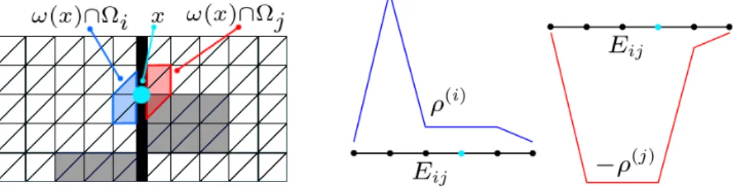
Figure 1 . Left: Visualization of the construction of an edge constraint in 2D for a given heterogeneous coefficient distribution. Middle: Maximum coefficient per finite element node of E

with respect to Ω

. Right: Maximum coefficient per finite element node of E

with respect to Ω

.

of heterogeneities, as shown by the numerical experiments in section 4 and section 5.

Please note that first results for diffusion problems in two dimensions using the new edge constraints instead of constraints resulting from the solution of a specific edge eigenvalue problem were already published in [23, 24].

3.1. Motivation and construction in two dimensions. Our new approach is strongly motivated by the generalized eigenvalue problem (2.8) from the adaptive coarse space [27, 49], which can equivalently be written as

hH(P D

v E

), K ij H(P D

w E

)i = µ ij hH(v E

), K ij H(w E

)i,

where K ij = diag(K ⁽ⁱ⁾ , K ^(j) ) and H(·) is the discrete harmonic extension from the interface of Ω i and Ω j to the interior of the subdomains Ω i and Ω j ; cf., e.g., [58, Sect. 4]. Therefore, as described in subsection 2.3.6, all eigenmodes with

µ ij = |H(P D

v E

)| K

|H(v _E

)| _K

> T OL (3.1)

are selected and then used to construct the adaptive constraints. In particular, this corresponds to the case where |H(P D

v E

)| K

is large, i.e., in the order of the con- trast of the coefficient function, while |H(v E

)| K

is small.

Now, in our new frugal approach, we propose a specific construction of v E

result- ing in the desired properties of the energies |H(P D

v E

)| K

and |H(v E

)| K

and therefore being a lower dimensional approximation of the original adaptive coarse space.

Let us first consider the case of diffusion in two dimensions. In this case, we only construct constraints corresponding to the edges of the domain decomposition.

We denote by E _ij the edge between two neighboring subdomains Ω _i and Ω _j and by ω(x) the support of the finite element basis functions associated with a finite element node x ∈ (Ω _i ∪ Ω _j ). For each x on ∂Ω _i or ∂Ω _j , respectively, we compute ρ b ⁽ⁱ⁾ (x) = max

y∈ω(x)∩Ω

ρ(y) and ρ b ^(j) (x) = max

y∈ω(x)∩Ω

ρ(y). Now, we define v ^(l) _E

ij

on ∂Ω l for l = i, j by

v _E ^(l)

ij

(x) :=

ρ b ^(l) (x), x ∈ ∂Ω l \Π ^(l) , 0, x ∈ Π ^(l) (3.2)

and v ^T _E

ij

:= (v ^(i)T _E

ij

, −v ^(j)T _E

ij

). Here, Π ^(l) denotes the index set of all local primal

variables. See also Figure 1 for a visualization of this function. As can be observed

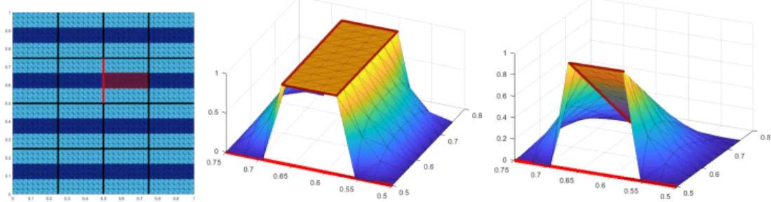
Figure 2. Visualization of the new constraints for a concrete coefficient distribution. Left:

Coefficient distribution with one channel associated with a high coefficient crossing each subdomain.

Dark blue corresponds to the high coefficient (1e6) and light blue to the low coefficient (1). Visualiza- tion for 4 × 4 subdomains and H/h = 9. Middle: Visualization of the discrete harmonic extension H(v

) for one floating subdomain. The visualized constraint leads to an energy of 17.49. Right:

Visualization of the discrete harmonic extension H(P

v

) for the same floating subdomain. The visualized constraint leads to an energy of 6.67e + 5.

exemplarily in Figure 2 (left) and Figure 3 (left), the energy |H(v E

)| K

is low.

On the other hand, the energy |H(P D

v E

)| K

is large for those two examples;

see in Figure 2 (right), where the energy is large due to the homogeneous Dirichlet boundary enforced by P D

, and Figure 3 (right), where the energy is large due to the gradient of the scaled jump P _D

v _E

on the edge.

We obtain the edge constraint by c _E

:= B _D

S _ij P _D

v _E

as in the adaptive coarse space; cf. subsection 2.3.6. We denote by B D

the submatrix of (B _D ⁽ⁱ⁾ , B _D ^(j) ) with the rows restricted to the edge E ij . We further define S ij = diag(S ⁽ⁱ⁾ , S ^(j) ), where S ⁽ⁱ⁾ and S ^(j) are the Schur complement matrices of K ⁽ⁱ⁾ and K ^(j) , respectively, with respect to the interface variables, as well as the operator P D

= B _D ^T

B ij .

The construction (3.2) can be further simplified by exploiting the fact that the scaled jumped operator P _D

is zero everywhere except on E _ij . Therefore, our new constraint is instead constructed as

v _E ^(l)

ij

(x) =

ρ b ^(l) (x), x ∈ E ij

0, x ∈ ∂Ω l \ E ij

(3.3)

for l = i, j; cf. the definition in [23]. In particular, due to the subsequent application of P D , both definitions of v _E ^(l)

ij

result in the same constraints c E

. For our parallel implementation, we use the latter definition of v _E ^(l)

ij

. There, we exploit the extension by zero to the remaining interface ∂Ω _l \ E _ij and reduce the applications of several P _D

to a few global applications of P _D ; see also section 5 for more details.

3.2. Diffusion in three dimensions. The respective case of diffusion problems in three dimensions is relatively analogous to the case of diffusion problems in two dimensions in subsection 3.1, with the main difference that we now compute our new constraint for faces F ij or, alternatively, closed faces F ij between neighboring subdomains Ω _i and Ω _j instead of edges E _ij . Let us first define

v _F ^(l)

ij

(x) =

ρ b ^(l) (x), x ∈ F ij ,

0, x ∈ ∂Ω _l \ F _ij ,

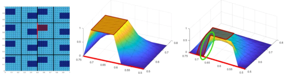
Figure 3 . Visualization of the new constraints for a concrete coefficient distribution. Left:

Coefficient distribution with boxes associated with a high coefficient. Dark blue corresponds to the high coefficient (1e6) and light blue to the low coefficient (1). Visualization for 4 × 4 subdomains and H/h = 8. Middle: Visualization of the discrete harmonic extension H(v

) for one floating subdomain, which is nearly constant in the area with a high coefficient marked in red. The visualized constraint leads to an energy of 17.39. Right: Visualization of the discrete harmonic extension H(P

v

) for the same floating subdomain, which has high gradients (see green ellipse) in the area with a high coefficient marked in red. The visualized constraint leads to an energy of 1.96e + 6.

and

v ^(l)

F

(x) =

ρ b ^(l) (x), x ∈ F ij , 0, x ∈ ∂Ω _l \ F _ij . (3.4)

Analogously to the two-dimensional case, we obtain our constraints c _F

ij

by applying B D

S ij P D

to either v F

or v _F

ij

, respectively. Let us remark that, due to the structure of the Schur complement matrix S ij as well as P D

, in both cases c _F

ij

can have nonzero entries on the closed face, i.e., on the open face F ij and on all edges E m , m = 1, 2, . . . , M belonging to the closed face F ij . We can therefore split a constraint c _F

ij

into a constraint c F

on the open face and constraints c E

, m = 1, ..., M , on the neighboring edges. The same approach of splitting the constraints into face- and edge-related parts is proposed in [27].

Depending on whether we also include the edge-related parts into the coarse space or not, four different possible variants of how we concretely enhance the coarse space related to faces exist:

FR1: Construct v ^T

F

for each closed face F _ij , and enforce both the edge-related parts c E

, m = 1, ..., M, as well as the part related to the open face of c F

. FR2: Construct v ^T _F

ij

for each closed face F ij , but just extract the terms of c F

related to the open face, while discarding the respective edge-related parts.

FR3: Construct v _F ^T

ij

for each open face F ij , and enforce both the edge-related parts c E

, m = 1, ..., M , as well as the part related to the open face of c F

. FR4: Construct v ^T _F

ij

for each open face F ij , but just extract the terms of c F

related to the open face, while discarding the respective edge-related parts.

We will compare the robustness of the four different variants in terms of condition number estimates and iteration counts in the numerical experiments in section 4. Let us remark that FR1 implements the complete constraints which are built analogously to the two-dimensional case. With respect to a parallel implementation, FR4 is the most promising, since the different open faces have no intersections with each other and therefore many local operations, such as, e.g., applications of P _D

, can be grouped to global operations and can be carried out for all faces at once; see section 5.

3.3. Linear elasticity in three dimensions. For the case of three-dimensional

linear elasticity problems, we know that, when applying the FETI-DP or BDDC

algorithm, we need six constraints, i.e., six rigid body modes, to control the null spaces for subdomains which have boundaries that do not intersect ∂Ω. For a generic domain Ω b with diameter H the basis for the null space ker(ε) is given by the three translations

(3.5) r 1 :=



 1 0 0



 , r 2 :=



 0 1 0



 , r 3 :=



 0 0 1



 ,

and the three linearrotations (3.6) r ₄ := 1

H





x 2 − b x 2

−x 1 + b x 1

0



 , r ₅ := 1 H





−x 3 + x b 3

0 x 1 − b x 1



 , r ₆ := 1 H



 0 x 3 − x b 3

−x 2 + b x 2



 ,

where x b ∈ Ω b is the center of the linear rotations; see, e.g., [38, Sect. 2]. We now construct six weighted constraints per face to obtain a robust coarse space. Basically, these constraints are based on the maximum coefficients per element, i.e., maximum Young modulus E > 0, as well as on the three translations and the three rotations for the respective face between two neighboring subdomains. Let us describe the concrete construction of the coarse constraints in some more detail. Let F ij be the open face between two neighboring subdomains Ω i and Ω j respectively, and F ij the closed face. For each finite element node x on ∂Ω i or ∂Ω j , we compute E b ^(l) (x) =

max

y∈ω(x)∩Ω

E(y) for l = i, j. Furthermore, we compute six scaled rigid body modes denoted by b r ^(l) m , m = 1, . . . , 6, l = i, j by pointwise scaling the rigid body modes r _m , m = 1, . . . , 6, with the respective vectors of maximum coefficients E b ^(l) (x), l = i, j.

Note that all three degrees of freedom belonging to a given node x ∈ ∂Ω _i ∪ ∂Ω _j are scaled with the same value of E b ^(l) (x) for l = i, j. For m = 1, . . . , 6 and l = i, j we then define

v _F ^(m,l)

ij

(x) =

b r m ^(l) (x), x ∈ F _ij 0, x ∈ ∂Ω _l \ F _ij (3.7)

Combining the vectors for both subdomains to v _F ^(m)T

ij

= (v _F ^(m,i)T

ij

, −v _F ^(m,j)T

ij

), we obtain the weights for the six face constraints as

(3.8) c ^(m)

F

:= B _D

S _ij P _D

v ^(m) _F

ij

, m = 1, . . . , 6.

The variants for closed faced are defined analogously; see also (3.4). Thus, the four different variants FR1 to FR4 of coarse spaces can be implemented as in the diffusion case. Please note that the resulting constraints can, in certain cases, be linearly depen- dent and thus result in less than six constraints per face. Therefore, we always apply a modified Gram-Schmidt algorithm after constructing the six aforementioned con- straints in our implementation. For the case of linear elasticity in two dimensions, the computation of c ^(m) _F

ij

, m = 1, . . . , 3, is completely analogous to the three-dimensional case. For two dimensions, we just scale all two dofs per node for a given node x with the same value of E b ^(l) (x) for l = i, j. Since the three-dimensional case is more general, we here chose to describe the three-dimensional case in more detail.

Due to the possible existence of hinge modes for two neighboring subdomains

in case of linear elasticity problems, using only face constraints and edge constraints

arising as a byproduct in the construction of the face constraints, as, e.g., in variants FR1 and FR3, might not always lead to a robust algorithm for complex coefficient distributions. In particular, in some cases the use of additional edge constraints is necessary to obtain moderate condition number bounds as well as scalabilty. We will consider such a coefficient distribution in Table 6, where the exclusive use of face constraints is not sufficient. For this special case, we enforce additional weighted edge constraints besides the weighted face and edge constraints already introduced. The construction of our weighted edge constraints is in principle completely analogous to the aforementioned face constraints. More precisely, the construction is basically the same except that we now operate on the index set of open edges between two neighbor- ing subdomains that do not share a face (alternatively, we can additionally construct weighted edge constraints for all edges, for simplicity, and finally apply a modified Gram-Schmidt algorithm to eliminate linearly dependent constraints). We thus ob- tain an additional variant, which we denote by FR5. Let us remark that we first use FR1 for all faces and ensure that we have no redundancies in the face-related and additional weighted edge constraints by applying a Gram-Schmidt orthogonalization.

3.4. Classic weighted average constraints in three dimensions. For com- parison, we also consider the classic coarse spaces introduced in [38], which we briefly describe in this subsection. We introduce weighted averages

(3.9)

P

x

∈X

ˆ

r j (x i )u(x i ) P

x

∈X

ˆ

r j (x i ) ² , j = 1, ..., l

on parts of the interface X , e.g., edges E or faces F. Here, we have l = 1 for the scalar diffusion case and l = 3 or l = 6 in the case of linear elasticity. Let us remark that in the latter case only five of the six constraints might be linear independent on straight edges; see [38]. For the scalar case, we consider the weights

ˆ

ρ(x) = max

y∈ω(x) ρ(y) and for the case of linear elasticity we choose

E(x) = max ˆ

y∈ω(x) E(y).

We further define pointwise

ˆ

r 1 (x) = ˆ ρ(x) in the scalar case and

ˆ

r _j (x) = ˆ E(x)r _j (x), j = 1, ..., 6

in case of linear elasticity, where r 1 , r 2 , and r 3 are the three translation and, respec- tively, r 4 , r 5 , and r 6 the three rotations; see also subsection 3.3. Let us remark that in [38] only weighted translations, i.e., ˆ r j , k = 1, ..., 3, have been used and thus the coarse space described in this subsection is in fact an extension of the robust coarse space used in [38].

4. Numerical results. In this section, we present numerical results obtained using our serial MATLAB implementations of the FETI-DP and BDDC algorithms.

We consider three-dimensional stationary diffusion and linear elasticity problems on

the unit cube, Ω = [0, 1] ³ , with Dirichlet boundary conditions on the left hand side

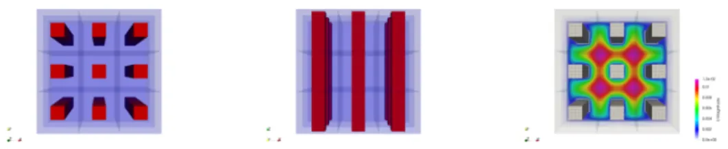
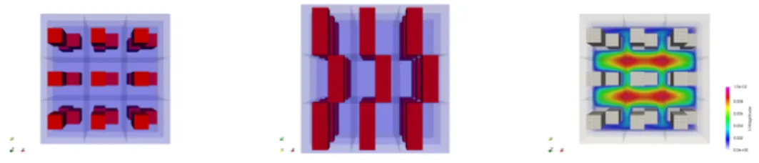
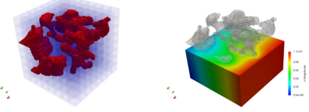
Figure 4 . Left and Middle: Coefficient function with one central beam per subdomain.

High coefficients are shown in red, and subdomains are shown in purple and by half-transparent slices. Right: Visualization of the corresponding solution for the stationary diffusion problem.

Visualization for 3 × 3 × 3 = 27 subdomains and H/h = 12.

of the boundary ∂Ω, i.e, ∂Ω D = 0 × [0, 1] ² . As already mentioned in subsection 2.3.4, we obtain the same quantitative condition number bounds for FETI-DP and BDDC since the two methods are dual to each other; see also [45, 48]. Therefore, we do not provide results for both methods for all tested coefficient distributions. We consider beams with high coefficients inside subdomains and with varying offsets between the subdomains as well as inclusions of high coefficients within subdomains.

Let us remark that, in addition to the considered face- or edge-based constraints, we always choose all vertices to be primal. In all tables and figures we use the following notation to distinguish between the different classic coarse spaces based on weighted averages:

e: Using vertex constraints and edge constraints (e), i.e., enforcing (3.9) for all edges E. In case of linear elasticity, only weighted translations are enforced, i.e., l = 3 in (3.9).

f: Using vertex constraints and face constraints (f), i.e., enforcing (3.9) for all faces F. In case of linear elasticity, only weighted translations are enforced, i.e., l = 3 in (3.9).

f + r: Using vertex constraints and face constraints (f), i.e., enforcing (3.9) for all faces F. In case of linear elasticity, translations and rotations (r) are enforced, i.e., l = 6 in (3.9).

4.1. Variations of one beam per subdomain. We provide numerical results for straight and shifted beams of high coefficients as shown in Figure 4 and Figure 5.

We consider both diffusion problems as well as linear elasticity problems and compare the results for our new frugal coarse space to the classic approach from [38]. For the straight channels which only cut through faces in Table 2, all four variants FR1 to FR4 show a more or less equivalent performance. Here, the classic approach also provides comparable and robust condition number bounds and iteration counts. For the shifted channels, see Table 3, the edge-related variants FR1 and FR3 show a slightly better performance compared to FR2 and FR4. This effect is mostly remarkable for the linear elasticity problems presented in Table 3. However, also the exclusively face- based variants FR2 and FR4 show robust condition numbers in all computations.

In particular, in this case, the classic weighted averages are not sufficient to provide robust algorithms. This shows that our new approach is indeed more general than classic averages and provides robustness for more complex coefficient distributions.

As a proof that our weighted constraints work equally well for the FETI-DP and the

BDDC algorithm, we further provide numerical results for the shifted channels and

the BDDC algorithm in Table 4.

Figure 5 . Left and Middle: Coefficient function with one beam per subdomain with offsets.

High coefficients are shown in red, and subdomains are shown in purple and by half-transparent slices. Right: Visualization of the corresponding solution for the stationary diffusion problem.

Visualization for 3 × 3 × 3 = 27 subdomains and H/h = 12.

new approach classic

N FR1 FR2 FR3 FR4 f

stationary diffusion

cond it cond it cond it cond it cond it 2 ³ 1.25 5 1.44 6 1.25 5 1.44 6 1.44 7 3 ³ 1.25 6 1.51 8 1.25 6 1.51 8 1.51 10 4 ³ 1.25 6 1.53 8 1.25 6 1.53 8 1.53 10

linear elasticity

cond it cond it cond it cond it cond it 2 ³ 1.59 10 2.70 13 1.59 10 2.71 14 2.71 14 3 ³ 1.63 11 2.78 16 1.62 10 2.78 16 2.78 15 4 ³ 1.63 11 2.86 16 1.62 10 2.85 16 2.85 16

Table 2

Condition numbers (cond) and iteration numbers (it) for the FETI-DP algorithm for stationary diffusion and linear elasticity problems in 3D with H/h = 6 for one straight beam per subdomain as in Figure 4. The higher coefficient is 1e6 and the lower coefficient is 1.

4.2. Inclusions within subdomains. Let us consider the case of inclusions of high coefficients within subdomains; see Figure 6. For the first set of experiments, we partition each subdomain into eight cubes of equal size and set a high coefficient in two of these cubes, which intersect only in a single vertex; see Figure 6. As the results in Table 5 show, our new face constraints lead to a robust algorithm for the diffusion problem for all variants FR1 to FR4. For elasticity problems, however, the resulting algorithm including only face constraints shows bad convergence behaviour or even diverges; see Table 6 (column 1). As a comparison, we further include results for an adaptive FETI-DP method in Table 6. Here, we use the adaptive coarse space as proposed by Mandel and Sousedík [49] and a variant thereof as implemented by Klawonn, Kühn, and Rheinbach [27]. Basically, in these methods the solution of certain local generalized eigenvalue problems on faces or edges is used to enrich the coarse space. We refer to [27,49] for more details on this adaptive method. In Table 6, we denote by:

• adaptive, face EVP: the adaptive FETI-DP method from [49] using exclu- sively eigenvalue problems on faces;

• adaptive, edge EVP: the adaptive FETI-DP method from [27], using ad- ditional eigenvalue problems on edges to enrich the coarse space.

As the results in Table 6 show, the adaptive FETI-DP algorithm also shows bad

new approach classic

N FR1 FR2 FR3 FR4 f

stationary diffusion

cond it cond it cond it cond it cond it

2 ³ 1.36 8 1.72 10 1.36 8 1.68 10 43 613.4 16 3 ³ 1.41 9 1.88 11 1.41 9 1.83 11 46 336.5 47 4 ³ 1.41 9 1.91 12 1.41 9 1.86 12 46 622.0 78

linear elasticity

cond it cond it cond it cond it cond it

2 ³ 1.92 12 3.92 18 1.90 13 3.68 17 37 930.9 54 3 ³ 1.90 12 4.48 19 1.89 12 4.37 19 68 238.5 124 4 ³ 1.92 12 4.91 21 1.90 12 4.76 21 76 027.6 264

Table 3

Condition numbers (cond) and iteration numbers (it) for the FETI-DP algorithm for stationary diffusion and linear elasticity problems in 3D with H/h = 6 for one beam per subdomain with offsets as in Figure 5. The higher coefficient is 1e6 and the lower coefficient is 1.

N FR1 FR2 FR3 FR4

stationary diffusion

cond it cond it cond it cond it 2 ³ 1.29 8 1.72 11 1.28 8 1.68 11 3 ³ 1.35 9 1.88 12 1.33 9 1.83 11 4 ³ 1.35 9 1.90 13 1.34 9 1.86 12

linear elasticity

cond it cond it cond it cond it 2 ³ 1.89 12 3.91 18 1.88 12 3.90 17 3 ³ 1.87 11 4.45 19 1.86 11 4.37 19 4 ³ 1.88 11 4.92 20 1.88 12 4.76 20

Table 4

Condition numbers (cond) and iteration numbers (it) for the BDDC algorithm for stationary diffusion and linear elasticity problems in 3D with H/h = 6 for one beam per subdomain with offsets as in Figure 5. The higher coefficient is 1e6 and the lower coefficient is 1.

convergence behavior for this specific linear elasticity problem when using exclusively

face constraints. However, the use of additional edge constraints again leads to a

robust algorithm, as the last column in Table 6 shows. This indicates that for this

specific coefficient distribution with two cubes of high coefficient per subdomain only

intersecting in a single vertex, a hinge mode exists in the case of linear elasticity, which

is not controlled by our new face constraints. Thus, we also consider the variant of

enforcing our new weighted edge constraints in addition to the already constructed

face average constraints, denoted by FR5; see subsection 3.3. In the second column

of Table 6, we present numerical results concerning this variant, given the inclusions

per subdomain intersecting only in a single vertex as before. Please note that the

additional use of explicit edge constraints in principle corresponds to the solution

of explicit edge eigenvalue problems for subdomains that do not share a face in the

context of the adaptive coarse space proposed in [27]. To obtain a robust algorithm,

we again use a modified Gram-Schmidt algorithm to eliminate all linearly dependent

constraints resulting from edge-related parts of weighted face constraints and the

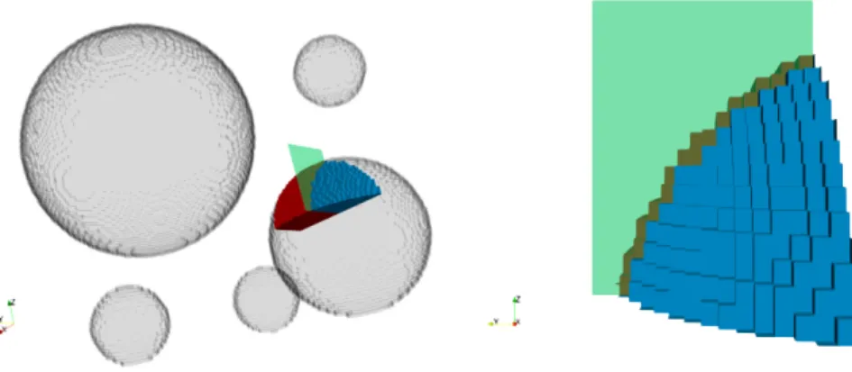
Figure 6 . Coefficient distribution with inclusions of high coefficients within subdomains. High coefficients are shown in red, and subdomains are shown by grey slices. Visualization for 3 × 3 × 3 subdomains and H/h = 12.

N FR1 FR2 FR3 FR4

stationary diffusion

cond it cond it cond it cond it 2 ³ 3.55 14 3.55 14 3.55 14 3.55 14 3 ³ 4.05 20 4.05 20 4.05 20 4.05 20 4 ³ 4.41 22 4.41 22 4.41 21 4.41 22

Table 5

Condition numbers (cond) and iteration numbers (it) for the FETI-DP algorithm for diffusion problems in 3D with H/h = 8 with two inclusions per subdomain as in Figure 6 (left). The higher coefficient is 1e6 and the lower coefficient is 1.

explicitly constructed edge constraints.

4.3. Reducing the coarse space dimension. As already stated above, our proposed coarse space is of a similar size as the classic coarse space introduced in [38].

In particular, we construct FR constraints over all faces and/or edges. However, for many real world problems, i.e., problems with realistic coefficient distributions, constraints on certain faces or edges are not necessary and can be omitted. Therefore, we further propose a modified variant to reduce the size of the coarse space, which only requires moderate additional effort.

Since our constraints are inspired from the eigenvalue problems introduced in [49, 50], we can use the quotient (3.1) corresponding to the eigenvalue problems to estimate the constraints actually required for a robust algorithm. Numerical results have shown that for faces or edges, for which the left side of the specific eigenvalue problem yields a high energy and the respective right side yields a low energy, additional coarse constraints are essential for robustness. For the convenience of the reader, we explicitly write down the right side (RS) and the left side (LS ) of the eigenvalue problem (2.8):

LS := P _D ^T

S ij P D

and RS := S ij .

See [49, 50, 54] for more technical details on the eigenvalue problem. To estimate the energy of our new constraints, we evaluate the product terms RSe := v _F ^T

RSv F

and LSe := v ^T _F

LSv F

in three dimensions, or RSe := v ^T _E

RSv E

and LSe :=

v _E ^T

ij

LSv E

in two dimensions, respectively. We further evaluate the ratio LSe/RSe

new approach adaptive approach

N FR1 FR5 face EVP edge EVP

linear elasticity

# c. cond it # c. cond it # c. cond it # c. cond it

2 ³ 288 25 158 54 324 1.72 10 39 58 679 58 173 3.70 15

3 ³ 1 452 18 530 180 1 668 1.73 10 164 87 156 246 838 3.42 20 4 ³ 4 032 19 626 232 4 680 1.74 10 429 114 882 471 2 319 3.44 20

Table 6

Condition numbers (cond), iteration numbers (it), and the size of the coarse space (# c.) for the FETI-DP algorithm for linear elasticity problems in 3D with H/h = 6 with two inclusions per subdomain as in Figure 6 (left). The higher coefficient is 1e6 and the lower coefficient is 1.

N FR2 FR2 red.

linear elasticity

# c. cond it # c. cond it 2 ³ 72 2.70 13 24 3.54 15 3 ³ 324 2.78 16 108 4.17 19 4 ³ 864 2.86 16 288 4.44 20

Table 7

Condition numbers (cond) and iteration numbers (it) for the FETI-DP algorithm for linear elasticity problems in 3D with H/h = 6 for one straight beam per subdomain as in Figure 4. Variant with reduced coarse space dimension. The higher coefficient is 1e6 and the lower coefficient is 1.

for all faces (and, depending on the chosen variant, for all edges). For the reduced dimensional variant, we now only integrate face constraints into the coarse space, for which the ratio LSe/RSe is above a user-defined tolerance T OL; see, e.g., [22]

for a discussion on the choice of T OL. We denote this reduced coarse space variant by FR2 red.. We show first numerical results concerning this reduced variant for straight channels in Table 7. For all shown cases, we are able to reduce the dimension of the coarse space to exactly one third of the original size while preserving both robust condition numbers and iteration counts. In Table 8, we further show numerical results for five spherical inclusions of different radii as depicted in Figure 11; see also section 5 for detailed parallel results concerning this specific coefficient distribution. For the diffusion case, we are able to reduce the size of the coarse space up to a factor of 2.4.

For the case of linear elasticity, the coarse space dimension is reduced by a factor of up to 1.6.

5. Parallel numerical results. We have added the new coarse space FR4 to our parallel BDDC implementation described in [32] and compare it with classic coarse spaces based on weighted edge or face translations and rotations as introduced in [38];

see also subsection 3.4. We again consider stationary diffusion and linear elasticity problems. Unless stated otherwise, Dirichlet boundary conditions on the complete boundary are used.

5.1. Parallel implementation and computational effort. Let us remark

that our PETSc-based parallel implementation presented in [32] is based on a BDDC

preconditioner for the complete system K g . Therefore, no Schur complement systems

are build explicitly. Consequently, we also avoid the computation of the matrix S ij ,

which is used for the construction of our edge or face constraints; see (3.8). Instead