Z → e τ and Z → µτ decayswiththeATLASdetector LeptonFlavourViolationattheLHC:asearchfor ATLASCONFNote

ATLAS-CONF-2020-035 11August2020

ATLAS CONF Note

ATLAS-CONF-2020-035

28th July 2020

Lepton Flavour Violation at the LHC : a search for Z → eτ and Z → µτ decays with the ATLAS

detector

The ATLAS Collaboration

In the Standard Model of particle physics, three lepton families (flavours) are part of the fundamental blocks of matter. All families have the same properties, except their mass. In addition, each family acts independently of the others, which is known as Lepton Flavour Conservation. Such conservation is assumed in the equations of the Standard Model, without a fundamental theoretical motivation. Since the formulation of the Standard Model, neutrino oscillation experiments have demonstrated that Lepton Flavour Conservation is violated in Nature. Yet, there is no experimental evidence that such violation occurs in processes involving only charged leptons. An observation of Lepton Flavour Violation among charged leptons would be an exciting sign of new particles or new interactions beyond the Standard Model.

The ATLAS experiment at the Large Hadron Collider at CERN sets a new strong constraint on Lepton Flavour Violation effects in weak interactions, searching for Z boson decays into a τ -lepton and another lepton of different flavour ( e or µ ) with opposite electric charge. Using a combination of LHC Run 1 and Run 2 proton-proton collision data, the branching fractions for these decays are now measured by the ATLAS experiment to be less than 9.5 × 10

( µτ ) and 8.1 × 10

( eτ ) at 95% confidence level, superseding the otherwise best limits set by the LEP experiments more than two decades ago.

© 2020 CERN for the benefit of the ATLAS Collaboration.

Reproduction of this article or parts of it is allowed as specified in the CC-BY-4.0 license.

In the Standard Model of particle physics (SM) [1–4], three quark and three lepton families (flavours) exist, which are replicas of particles with the same properties except for their mass. The number of leptons in each family is conserved in interactions, and the violation of this assumption is known as Lepton Flavour Violation (LFV). LFV is not possible in the SM, even though no fundamental principles forbid it. The observation of neutrino oscillations, where neutrinos (the neutral leptons) of one flavour transform into that of another [5, 6], indicates that LFV processes do occur in Nature. It reveals that neutrinos have mass, and this constitutes the first experimental evidence of new phenomena beyond those originally predicted by the SM. These observations open new questions, such as why neutrino masses are so small compared to the charged leptons, or why the neutrino flavour mixing is much larger than the quark flavour mixing.

An observation of LFV in charged lepton interactions would be another unambiguous sign of new physics.

In particular, decays of the Z boson into an electron or muon and a τ -lepton are of experimental interest because of the abundance of Z bosons produced at the Large Hadron Collider (LHC), and the weaker experimental constraint on these final states than on the other possible LFV decay, Z → e µ [7]. According to our current knowledge, these decays can occur only via neutrino mixing and are too rare to be detected.

For instance, only one in approximately 10

Z bosons would decay into a muon and a τ -lepton [8]. An observation of such decays would, therefore, require new theoretical explanations. For example, theories that predict the existence of heavy neutrinos [9], which provide a fundamental understanding of the tiny masses and large mixing of the active neutrinos observed, predict LFV involving τ -leptons in up to one in 10

Z decays. The ATLAS experiment can help to determine or narrow down the mass and interaction strength of new particles, such as those hypothesised to explain neutrino properties [9], by observing or setting ever more stringent constraints on LFV Z decays.

Constraints on the branching fraction ( B ) of the LFV decays of the Z boson involving a τ -lepton have been set by the LEP experiments: B(Z → eτ) < 9 . 8 × 10

[10] and B(Z → µτ) < 1 . 2 × 10

[11] at 95%

confidence level (CL). The ATLAS experiment [12] at the LHC has set a constraint B(Z → µτ) < 1 . 3 × 10

at 95% CL using Run 1 and part of Run 2 data, and B(Z → eτ) < 5 . 8 × 10

using part of Run 2 data [13].

The work presented here uses proton–proton ( pp ) collision data collected by the ATLAS experiment during the LHC Run 2, containing about eight billion Z boson decays. Only events with a τ -lepton that decays hadronically are considered. Neural network classifiers are used in a novel way for optimal discrimination of signal from backgrounds and improved sensitivity in the measurement of LFV effects from the data using a binned maximum-likelihood statistical fit. The LHC Run 2 result is combined with a previous LHC Run 1 result to further improve sensitivity.

These results set stringent constraints on LFV Z decays involving τ -leptons, superseding the otherwise most stringent ones set by the LEP experiments more than two decades ago.

1 The ATLAS experiment and data sample

To record and analyse the LHC pp collisions, the ATLAS experiment [12, 14, 15] uses a multipurpose particle detector with a forward–backward symmetric cylindrical geometry and a near 4 π coverage in solid angle1. It consists of an inner tracking detector (ID) surrounded by a thin superconducting solenoid

1ATLAS uses a right-handed coordinate system with its origin at the nominal interaction point (IP) in the centre of the detector and thez-axis along the proton beam direction. Thex-axis points from the IP to the centre of the LHC ring, and they-axis points upwards. Cylindrical coordinates (r,φ) are used in the transverse plane,φbeing the azimuthal angle around thez-axis.

providing a 2 T axial magnetic field, electromagnetic (EM) and hadronic calorimeters, and a muon spectrometer (MS). The ID covers the pseudorapidity range |η| < 2 . 5. It consists of silicon pixel, silicon microstrip, and transition radiation tracking detectors. Lead/liquid-argon (LAr) sampling calorimeters provide EM energy measurements with high granularity. A steel/scintillator-tile hadronic calorimeter covers the central pseudorapidity |η | < 1 . 7. Higher pseudorapidities range, up to |η| < 4 . 9, are instrumented with LAr calorimeters for EM and hadronic energy measurements. The MS surrounds the calorimeters and is based on three large air-core toroidal superconducting magnets with eight coils each. The field integral of the toroids ranges between 2.0 and 6.0 Tm across most of the detector. The MS includes a system of precision tracking chambers and fast detectors for triggering. A two-level trigger system is used for the real-time selection of the pp collisions to be recorded for offline analysis [16]. The first-level trigger is implemented in hardware, and analyses 40 MHz of pp collisions using a subset of the detector information, reducing the rate to about 100 kHz. This is followed by the software-based high-level trigger, which reduces the event selection rate to about 1 kHz.

The data used are pp collisions (in the following denoted as “events”) from the LHC at 13 TeV in the years 2015-2018, corresponding to an integrated luminosity of 139 fb

(for events passing data quality criteria) and recorded using single electron and muon triggers [16]. For the search in the µτ channel, combination with the results of a similar search on pp collisions at 8 TeV from the years 2011-2012, corresponding to an integrated luminosity of 20.3 fb

, is performed.

Electron candidates are reconstructed from energy deposits in the electromagnetic calorimeter associated with a charged-particle track measured in the inner detector. They are required to pass the Medium likelihood-based identification selection [17], to have transverse momentum (momentum in the plane perpendicular to the proton beam line) p

> 30 GeV, and pseudorapidity |η| < 1 . 37 or 1 . 52 < |η| < 2 . 47.

Muon candidates are constructed by matching an inner detector track with a track reconstructed in the muon spectrometer, are required to have p

> 30 GeV and |η| < 2 . 5 and to pass the Medium muon identification requirements [18]. Both electron and muon candidates satisfy the Tight isolation requirements [17, 18], which uses calorimeter-based and track-based isolation criteria. The lower thresholds on the muon and electron transverse momenta are driven by the acceptance of the trigger selection.

Jets are reconstructed by clustering energy deposits in the calorimeter using the anti- k

algorithm [19, 20] with the radius parameter R = 0 . 4. The measured jet transverse momentum is corrected for detector effects by weighting energy deposits arising from electromagnetic and hadronic showers differently [21].

To reduce the contamination from jets from the additional pp collisions occurring in the same proton bunch crossing (pileup), the Medium “Jet Vertex Tagger” (JVT) algorithm decision is applied [22]. Jets fulfilling p

> 20 GeV and |η| < 2 . 5 are identified as containing b -hadrons if tagged by a multivariate algorithm [23].

The visible decay products of the hadronic decay of a τ -lepton are reconstructed as a τ

candidate, from a jet with p

> 10 GeV, |η | < 1 . 37 or 1 . 52 < |η| < 2 . 5, formed using the anti- k

algorithm with parameter R = 0 . 4. The τ

candidates identification is performed by a recurrent neural network algorithm [24] using calorimetric shower shapes and tracking information as input variables; the algorithm allows to discriminate τ

candidates with one or three associated tracks from quark- or gluon-initiated jets. These candidates are also called “1-prong” (1P) and “3-prong” (3P) respectively. τ

candidates are required to pass the Tight identification selection, which has an efficiency of 60% (45%) for true 1P (3P) τ

candidates, and a misidentification rate of one in 70 (700) for fake 1P (3P) candidates in dijet events.

The pseudorapidity is defined in terms of the polar angleθasη=−ln tan^θ₂. The angular distance between two detected particle candidates is measured in units of∆R≡p

(∆η)2+(∆φ)2.

Dedicated multivariate algorithms are used to further discriminate τ

against electrons and to calibrate the τ

energy [25]. Final τ

candidates are required to have p

> 25 GeV. The τ

candidate with the largest p

in each event is considered to be the final candidate and is required to have p

> 25 GeV.

In Z → `τ decays the τ

candidate is expected to be correctly selected 98% of the time.

The missing transverse momentum is calculated as the negative vectorial sum of the p

of all fully calibrated and reconstructed physics objects [26, 27]. The calculation also includes inner detector tracks that originate from the vertex associated with the hard-scattering process but are not associated with any of the reconstructed objects. The missing transverse momentum ( E

T

) is defined as the magnitude of this vector, and is the best proxy for the total transverse momentum of neutrinos in an event.

2 Search strategy

The Z → `τ → `τ

+ ν ( ` = e, µ ) signal events have a number of key features that can be exploited to separate them from the SM background events.

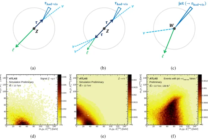
The signal events are characterised by their unique final state which has exactly one light lepton ` and one τ -lepton, with the invariant mass of the pair compatible with the Z boson mass. The ` and τ particles carry opposite-sign charges and are emitted back-to-back (on average) in the plane transverse to the proton beam direction. Since the τ -lepton is typically boosted due to the large difference between its mass and its parent Z boson mass, the neutrino from the τ decay in a signal event is collinear (on average) with the τ

candidate in the transverse plane. The neutrino escapes the detector without interacting with it, and is reconstructed as part of the E

T

of the event. In a signal event, this is the only major source of E

T

.

Major background contributions for this search are: lepton-flavour-conserving Z → ττ → `τ

+ 3 ν decays, where one of the τ -leptons decays leptonically and the other hadronically; Z → `` decays, where one of the light leptons is misidentified as the τ

candidate; and events with a quark- or gluon-initiated jet that is misidentified as the τ

candidate (hereafter referred to as events with “fakes”), which are predominantly W(→ `ν) +jets events and purely hadronic multijet events. Other SM processes with a real

`τ

final state, such as decays of top quarks, two gauge bosons or a Higgs boson, and those with a real τ

but a jet misidentified as a light lepton, such as W(→ τν) +jets, are considered although their contribution to the overall background is minor.

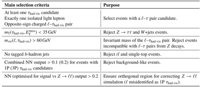
The signal and background events are first separated by a set of event selection criteria that help define the signal region (SR). The main selection criteria are summarised in Table 1. They are primarily based on the multiplicity of reconstructed particle candidates and the event topology, in particular the transverse masses ( m

), which are defined as

m

(X, E

T

) ≡

r

2 · p

( X) · E

T

·

1 − cos (φ

− φ

)

, (1) where X is either a light lepton or a τ

candidate. A schematic illustration of the expected signal and background topologies is shown in Figure 1.

Subsequently, binary neural network (NN) classifiers trained on simulated events, are used to distinguish

signal events from W +jets, Z → ττ and Z → `` background events. Each individual NN is optimised to

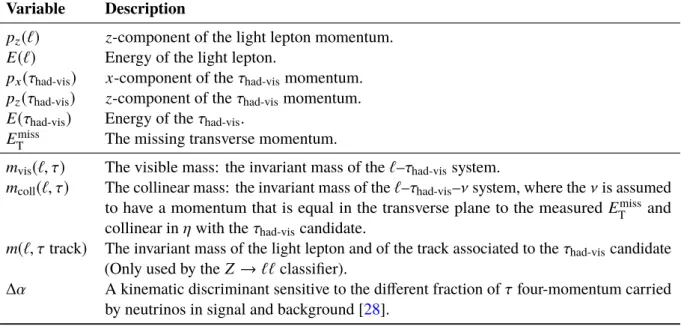
discriminate against a single background process. The input to these NNs is a mixture of low-level and

high-level kinematic variables, as shown in Table 2. For optimal training, the frame of reference in which

(a) (b) (c)

0 20 40 60 80 100 120 140

) [GeV]

miss ET µ, T( m 0

20 40 60 80 100 120 140 ) [GeV]miss TE, τ(Tm

0 0.001 0.002 0.003 0.004 0.005 0.006 ATLAS

Simulation Preliminary = 13 TeV s

τ µ

→ Z Signal

(d)

0 20 40 60 80 100 120 140

) [GeV]

miss ET µ, T( m 0

20 40 60 80 100 120 140 ) [GeV]miss TE, τ(Tm

0 0.0005 0.001 0.0015 0.002 0.0025 0.003 ATLAS

Simulation Preliminary = 13 TeV s

τ τ

→ Z

(e)

0 20 40 60 80 100 120 140

) [GeV]

miss ET µ, T( m 0

20 40 60 80 100 120 140 ) [GeV]miss TE, τ(Tm

0 0.0002 0.0004 0.0006 0.0008 0.001 0.0012 ATLAS

Preliminary = 13 TeV, 139 fb-1

s

fakes had-vis

τ

→ Events with jet

(f)

Figure 1: A schematic representation of the typical topology of a(a)signalZ →`τ,(b)Z → ττor(c)W+jets event selected in the SR, as seen in the plane transverse to the beam line. The green arrows represent reconstructed light leptons (`). The blue triangles represent theτ_had-viscandidates. The light blue dashed lines represent neutrinos that escape detection and are reconstructed as (part of) the missing transverse momentum of the event. The two-dimensional histograms show the distributions ofm_T(τ_had-vis,E^miss

T )versusm_T(µ,E^miss

T )of(d)simulatedZ→ µτ events,(e)simulatedZ →ττevents and(f)events measured in data in regions where quark- or gluon-initiated jets are misidentified asτ_had-viscandidates (events with jet→τ_had-visfakes) in theµ–τ_had-visfinal state. The colour map represents the fraction of events in each bin.

Table 1: Main selection criteria for events in the signal region.

Main selection criteria Purpose

At least one τ

candidate

Select events with a ` – τ pair candidate.

Exactly one isolated light lepton Opposite-sign charged ` – τ

pair m

(τ

, E

T

) < 35 GeV Reject Z → ττ and W +jets events.

m

(`, τ

) > 60 GeV Invariant mass of the ` – τ

pair. Reject events incompatible with ` – τ pairs from Z decays.

No tagged b -hadron jets Reject t t ¯ and single-top events.

Combined NN output > 0.1 (0.2) for events with 1P (3P) τ

candidates

Reject background-like events.

NN (optimised for signal vs Z → `` ) output > 0.2 Ensure orthogonal region for correcting Z → ``

simulation ( ` misidentified as 1P τ

).

the first six, low-level variables are measured is chosen such that known spatial symmetries are removed.

They are measured in a boosted and rotated frame of reference where the transverse momentum of the

` – τ

– E

T

system is zero and the E

T

is aligned with the positive x -axis. The last four, high-level variables are measured in the laboratory frame.

The high-level variables help the NNs to converge faster while they exploit any residual correlations between the low-level variables. The outputs from the individual NNs are numbers between zero and one that reflects the likelihood for an event to be a signal event, and are combined into a final discriminant, hereafter referred to as the “combined NN output”. The combination is parametrised by weights associated to each individual NN and the weights are optimised for the discrimination among different background processes along the combined NN output value. This allows the maximum-likelihood fit to determine more precisely the background contributions, which ultimately improves the sensitivity.

Events classified by the NNs to be extremely background-like are excluded from the SR, as indicated in Table 1. The signal acceptance times efficiency in the SR is 2.7% for the eτ channel and 3.0% for the µτ channel, as determined from simulated signal samples.

3 Signal and background predictions

Predictions for signal and background contributions to the event yield in the SR are based partly on Monte Carlo (MC) simulations and partly on the use of data in regions that are orthogonal to the SR and enriched in background events. The method for making the predictions is similar to that detailed in the early Run 2 search [13].

The signal events were simulated using Pythia 8 [29] with matrix elements calculated at leading-order (LO)

in the strong coupling constant ( α

). Parameters for initial-state radiations, multiparton interactions and beam

remnants are set according to the A14 [30] set of tuned parameters (tune) with the NNPDF2.3LO Parton

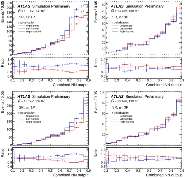
Distribution Function (PDF) set [31]. Nominal signal MC samples are generated with a parity-conserving

Z `τ vertex and unpolarised τ -leptons. The scenarios where the decays are maximally parity-violating are

Table 2: Input variables for the neural network classifiers. The first six variables are the low-level variables, which are measured in the boosted and rotated frame as described in the text. The last four variables are the high-level variables, which are measured in the laboratory frame.

Variable Description

p

(`) z -component of the light lepton momentum.

E(`) Energy of the light lepton.

p

(τ

) x -component of the τ

momentum.

p

(τ

) z -component of the τ

momentum.

E(τ

) Energy of the τ

. E

T

The missing transverse momentum.

m

(`, τ) The visible mass: the invariant mass of the ` – τ

system.

m

(`, τ) The collinear mass: the invariant mass of the ` – τ

– ν system, where the ν is assumed to have a momentum that is equal in the transverse plane to the measured E

T

and

collinear in η with the τ

candidate.

m(`, τ track ) The invariant mass of the light lepton and of the track associated to the τ

candidate (Only used by the Z → `` classifier).

∆ α A kinematic discriminant sensitive to the different fraction of τ four-momentum carried by neutrinos in signal and background [28].

considered by reweighting the simulated unpolarised events with TauSpinner [32]. It calculates as event weights the chance of occurrence of every generated signal event, based on their kinematics, under the assumption of a specific τ polarisation state.

MC samples for Z → ττ events were simulated with Sherpa 2.2.1 [33] generator using the NNPDF 3.0 NNLO PDF set [34] and next-to-leading-order (NLO) matrix elements for up to two partons, and LO matrix elements for up to four partons calculated with the Comix [35] and OpenLoops [36–38] libraries.

They were matched with the Sherpa parton shower [39] using the MEPS@NLO prescription [40–43]

with the set of tuned parameters developed by the Sherpa authors. The Z → `` samples were generated using Powheg+Pythia 8 [29, 44] with NLO matrix elements. The CT10 PDF set [45] is used for the hard-scattering processes, whereas the CTEQ6L1 PDF set [46] and the parameters set according to the AZNLO tune [47] are used for the parton shower.

All MC samples include a detailed simulation of the ATLAS detector with Geant 4 [48], to produce predictions that can be directly compared with the data. Furthermore, simulated inelastic pp collisions, generated with Pythia 8 using the NNPDF2.3LO PDF set and the A3 [49] tune, are overlaid to model additional, pileup collisions. Simulated events are reweighted to model the pileup conditions of a given data taking period. All simulated events were processed using the same reconstruction algorithms as used in data.

The accuracy and precision of the prediction of signal, Z → ττ and Z → `` events are improved through corrections to the MC simulations derived from measurements in data. The simulated transverse momentum spectra of the Z bosons are reweighted to match the unfolded distribution measured by ATLAS in Ref. [50].

This improves the Z -boson production simulation, which is done at different orders in α

using different

MC generators. It also reduces the uncertainties related to missing higher orders in α

. The predicted

overall yields of signal and Z → ττ events are determined by a binned maximum-likelihood fit to data

(Section 4) in the SR and in a control region enhanced with Z → ττ → `τ

+ 3 ν events (CRZ ττ ),

more precisely than the predictions from pure simulations. The predicted signal and Z → ττ yields are scaled by a common unconstrained parameter, which accounts for theoretical uncertainties on the total Z -boson production cross section, as well as the experimental uncertainties related to the acceptance of the common `τ

final state. The selection criteria for events in the CRZ ττ are the same as that for events in the SR, except that events are required to have m

(τ

, E

T

) > 35 GeV, m

(`, E

T

) < 40 GeV, and m

(`, τ) that falls between 70 GeV and 110 GeV.

Much smaller contributions to the total background originate from Z → `` events. Their overall yield is predicted based on the measured value of σ(Z ) [51] times the measured integrated luminosity. The uncertainties in these two ATLAS measurements are taken into account. The predicted misidentification rate of electrons or muons in Z → `` events are corrected using data in a region enriched in Z → `` events and orthogonal to the SR (CRZ `` ), where the last selection criterion in Table 1 is inverted and the outputs of the Z ττ and the Wjets NN classifiers are larger than 0.8. The correction is derived as a function of p

and |η| of the τ

candidate. Statistical uncertainties in the correction are considered.

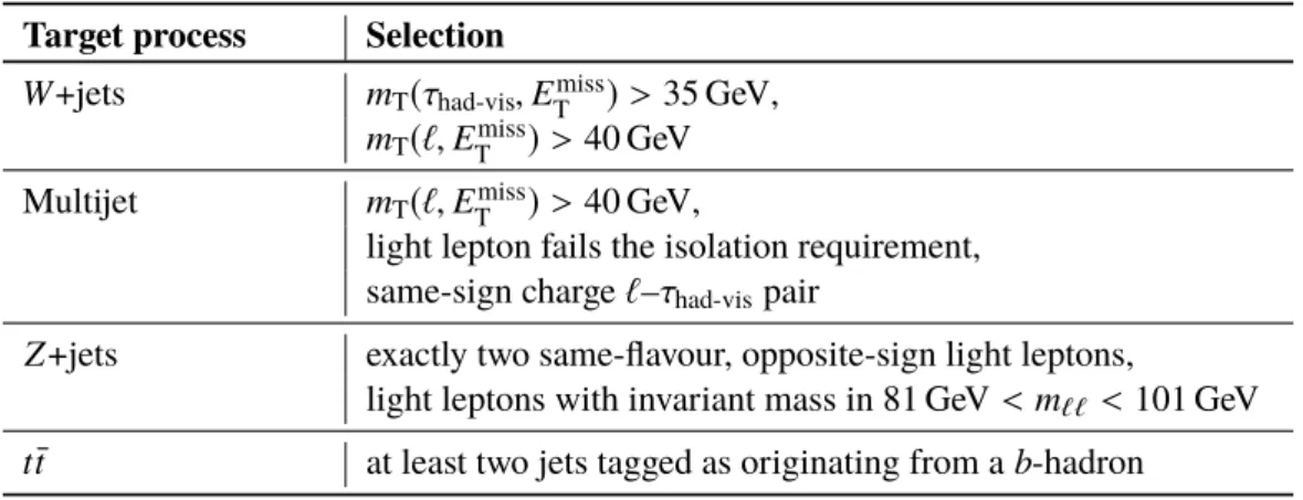
Table 3: Selection criteria for the fakes-enriched regions. Listing only those criteria that differ from the selection in the SR.

Target process Selection W +jets m

(τ

, E

T

) > 35 GeV, m

(`, E

T

) > 40 GeV Multijet m

(`, E

T

) > 40 GeV,

light lepton fails the isolation requirement, same-sign charge ` – τ

pair

Z +jets exactly two same-flavour, opposite-sign light leptons,

light leptons with invariant mass in 81 GeV < m

< 101 GeV t¯ t at least two jets tagged as originating from a b -hadron

Events where quark- or gluon-initiated jets are misidentified as τ

candidates are one of the dominant contributions to the background, and are estimated from data using the “fake-factor method” which is also described in Ref. [13]. A fake factor is defined as the ratio of the number of events with a fake 1P or 3P τ

candidate passing the Tight tau identification requirement to those failing it. Four fake factors, one for each of the most important backgrounds with fakes ( W (→ `ν) +jets, multijet, Z +jets and t t ¯ events), are measured in data in fakes-enriched regions (FR) with high concentration of a background type. These regions are orthogonal to any of the regions used for the final maximum-likelihood fit. The selection criteria for events in the FRs are summarised in Table 3. The fake factors are measured as functions of the transverse momentum of the τ

candidate, separately for eτ and µτ events and for events with 1P or 3P τ

candidates.

The number of events with a fake 1P or 3P τ

candidate in a given region is estimated by the amount of events with a τ

candidate failing the Tight tau identification requirement, but otherwise passing all other selection criteria for that region, multiplied by an average of the fake factors. To calculate this average, the fake factors are summed with weights equal to the expected relative contribution of the corresponding background to the total yield of events in the region with the inverted tau identification requirement [13].

This approach is used to model the kinematic properties of the events with fakes. The total predicted yields

of these events in the SR and CRZ ττ are instead determined by a maximum-likelihood fit, separately

for events with 1P and 3P τ

candidates. This data-driven approach avoids the theory uncertainties associated to simulating misidentified τ

candidates, and makes full use of the large amount of data collected.

The remaining background processes (the “Others” background), which have relatively small contributions in the SR, are estimated using MC simulations. They include events from t¯ t , single-top, Wt , and gluon- fusion and vector-boson-fusion Higgs productions that are simulated using Powheg+Pythia, and events from W(→ τν) +jets and diboson productions that are simulated using Sherpa. The yields of these events are normalised to the theoretical cross sections.

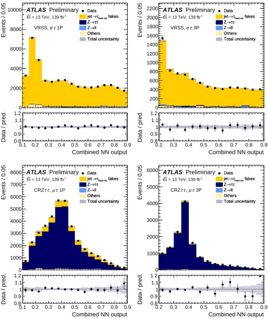
The modelling of the background is validated using events in regions where signal contamination is negligible. Especially important to the search is the modelling of the combined NN output distribution of Z → ττ events and events with fakes. The modelling is validated by comparing the predicted distributions with data respectively in the CRZ ττ and in a region similar to the SR kinematics but with events that have same-charge ` – τ

pairs (VRSS), as shown in Figure 2.

4 Constraints on B( Z → `τ )

A statistical analysis of the selected events is performed in order to assess the presence of LFV signal events.

The statistical method is the same as that used in Ref. [13]. A simultaneous binned maximum-likelihood fit to the combined NN output in the SR and the collinear mass in the CRZ ττ is used to constrain uncertainties in the models and extract evidence of a possible signal. The fit is performed independently for the eτ and µτ channels. Events with 1P and 3P τ

candidates are considered separately. Hypothesis tests, in which the log-likelihood ratio is used as the test statistic, are used to assess the compatibility between the background and signal models and the data.

There are four unconstrained parameters in the fits: two of them determine the overall yields of events with fake 1P τ

or 3P τ

candidates; one determines σ(Z) times the overall acceptance and reconstruction efficiency of events with true `τ

final state ( Z → ττ and signal); and one determines the LFV branching fraction B(Z → `τ) , which is the parameter of interest in the fit.

Constrained parameters are also introduced to account for systematic uncertainties in the signal and background predictions. In case of no significant deviations from the SM background, exclusion limits are set using the CL

method [52].

Fitting the data in the CRZ ττ and in the low combined NN output value region (where no signal is present) benefits the overall sensitivity of the fit to the signal because it reduces the uncertainties of the background model in the high combined NN output value region, where the majority of the signal is expected.

Systematic uncertainties in this search include uncertainties in the MC modelling of trigger, reconstruction,

identification and isolation efficiencies, as well as energy calibrations and resolutions of reconstructed

objects. Theory uncertainties in the predicted cross sections are also assigned to the background processes,

except events with Z bosons and events with fakes whose yields are determined from data. These

events constitute only a small fraction of the background events in the SR and are assigned conservative

uncertainties in the range between 4% to 20%. The dominant uncertainties in this search are those in the

overall yields of event with fakes, which are predominantly of statistical nature, and those in the τ

energy calibration, which are constrained by the fit of the collinear mass spectrum to the data in the CRZ ττ .

obs_x_SS_SR_el_1P_NN_output_comb__times__1

0 2000 4000 6000 8000 10000

Events / 0.05

Data fakes

had-vis

τ

→ jet

τ τ

→ Z

→ll Z Others Total uncertainty Data

fakes

had-vis

τ

→ jet

τ τ

→ Z

→ll Z Others Total uncertainty

Preliminary ATLAS

= 13 TeV, 139 fb-1

s

τ 1P e VRSS,

0.1 0.2 0.3 0.4 0.5 0.6 0.7 0.8 0.9 Combined NN output 0.8

0.9 1 1.1 1.2

Data / pred.

obs_x_SS_SR_el_3P_NN_output_comb__times__1

0 200 400 600 800 1000 1200 1400 1600 1800 2000 2200

Events / 0.05

Data fakes

had-vis

τ

→ jet

τ τ

→ Z

→ll Z Others Total uncertainty Data

fakes

had-vis

τ

→ jet

τ τ

→ Z

→ll Z Others Total uncertainty

Preliminary ATLAS

= 13 TeV, 139 fb-1

s

τ 3P e VRSS,

0.2 0.3 0.4 0.5 0.6 0.7 0.8 0.9 Combined NN output 0.8

0.9 1 1.1 1.2

Data / pred.

obs_x_CRZtt_mu_1P_NN_output_comb__times__1

0 1000 2000 3000 4000 5000 6000 7000 8000

Events / 0.05

Data fakes

had-vis

τ

→ jet

τ τ

→ Z

→ll Z Others Total uncertainty Data

fakes

had-vis

τ

→ jet

τ τ

→ Z

→ll Z Others Total uncertainty

Preliminary ATLAS

= 13 TeV, 139 fb-1

s

τ 1P µ τ, τ CRZ

0.1 0.2 0.3 0.4 0.5 0.6 0.7 0.8 0.9 Combined NN output 0.8

0.9 1 1.1 1.2

Data / pred.

obs_x_CRZtt_mu_3P_NN_output_comb__times__1

0 1000 2000 3000 4000 5000 6000

Events / 0.05

Data fakes

had-vis

τ

→ jet

τ τ

→ Z

→ll Z Others Total uncertainty Data

fakes

had-vis

τ

→ jet

τ τ

→ Z

→ll Z Others Total uncertainty

Preliminary ATLAS

= 13 TeV, 139 fb-1

s

τ 3P µ τ, τ CRZ

0.2 0.3 0.4 0.5 0.6 0.7 0.8 0.9 Combined NN output 0.8

0.9 1 1.1 1.2

Data / pred.

Figure 2: The best-fit (see Section4) expected and observed distributions of the combined NN output in the VRSS for theeτchannel (top row) and in the CRZττfor theµτchannel (bottom row) for events with 1P or 3Pτ_had-vis candidates. In the panels below each plot, the ratios of the observed yields to the best-fit background yields are shown. The hatched error bands represent the combined statistical and systematic uncertainties. The last bin in each plot includes overflow events.

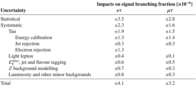
A summary of the uncertainties and their impact on the best-fit LFV branching fraction is given in Table 4, which shows that the sensitivity of the search is primarily limited by the available amount of data.

Table 4: A summary of the uncertainties and their impacts on the signal branching fraction. The uncertainties for light lepton include those in the trigger, reconstruction, identification and isolation efficiencies, as well as energy calibrations. The uncertainties for jet andE^miss

T include those in the energy calibrations and resolutions.

Impacts on signal branching fraction [×10

]

Uncertainty eτ µτ

Statistical ± 3.5 ± 2.8

Systematic ± 2.3 ± 1.6

Tau ± 1.9 ± 1.5

Energy calibration ± 1.3 ± 1.4

Jet rejection ± 0.3 ± 0.3

Electron rejection ± 1.3

Light lepton ± 0.4 ± 0.1

E

T

, jet and flavour tagging ± 0.6 ± 0.5

Z background modelling ± 0.7 ± 0.3

Luminosity and other minor backgrounds ± 0.8 ± 0.3

Total ± 4.1 ± 3.2

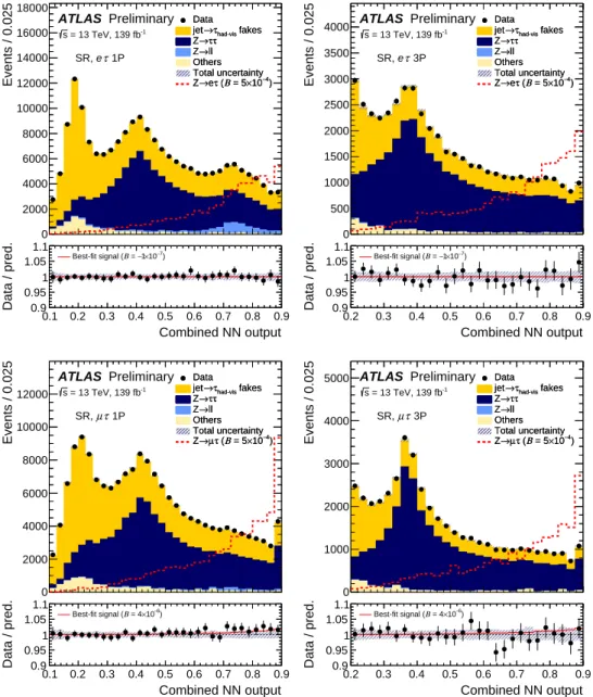
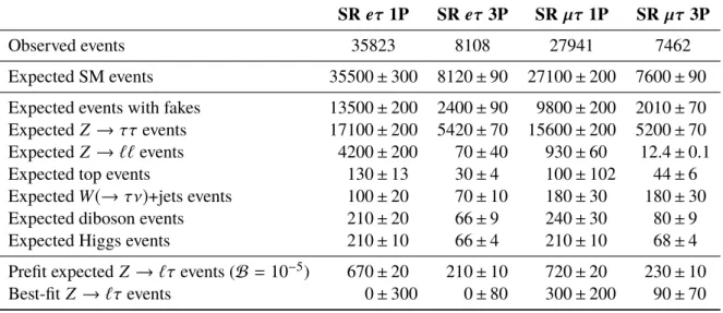
The best-fit expected and observed distributions of the combined NN output in the SR are shown in Figure 3. The best-fit yields of Z → ττ and events with fakes are close to the prefit predicted values and are determined with a relative precision between 2% to 4%. Table 5 shows the best-fit expected background and signal yields and the observed number of events in the SR of the eτ and µτ channels with an additional requirement of combined NN output > 0 . 7 to consider the most signal-like events.

The amount of best-fit Z → `τ signal in 139 fb

Run 2 data corresponds to the branching fractions2 B(Z → eτ) = (− 0 . 1 ± 3 . 5 ( stat )± 2 . 3 ( syst ))× 10

and B(Z → µτ) = ( 4 . 3 ± 2 . 8 ( stat )± 1 . 6 ( syst ))× 10

. No statistically significant deviation from the SM prediction is observed and upper limits on the LFV branching fractions are set. For the µτ channel, a more stringent upper limit is set by combining the likelihood functions of the presented measurement with a similar measurement done with ATLAS Run 1 data [53]. Nuisance parameters from the two measurements are considered uncorrelated in the combined likelihood function. The upper limits are shown in Table 6 for the hypotheses of LFV decays involving parity-conserving, and maximally parity-violating, interactions.

These results set stringent constraints on LFV Z decays involving τ -leptons (using only their hadronic decays), superseding the otherwise most stringent ones set by the LEP experiments more than two decades ago. The precision of this result is dominated by statistical uncertainties.

2While the actual physical branching ratio must be positive, the signal strength modifier in the fit is not constrained to be positive.

obs_x_SR_el_1P_NN_output_comb

0 2000 4000 6000 8000 10000 12000 14000 16000 18000

Events / 0.025

Data fakes

had-vis

τ

→ jet→ττ Z

→ll Z Others Total uncertainty

4) 10−

× Β = 5 τ (

→e Z Data

fakes

had-vis

τ

→ jet→ττ Z

→ll Z Others Total uncertainty

4) 10−

× Β = 5 τ (

→e Z

Preliminary ATLAS

= 13 TeV, 139 fb-1

s τ 1P e SR,

0.1 0.2 0.3 0.4 0.5 0.6 0.7 0.8 0.9 Combined NN output 0.9

0.95 1 1.05 1.1

Data / pred.

7) 10−

1× = − Β Best-fit signal (

obs_x_SR_el_3P_NN_output_comb

0 500 1000 1500 2000 2500 3000 3500 4000

Events / 0.025

Data fakes

had-vis

τ

→ jet→ττ Z

→ll Z Others Total uncertainty

4) 10−

× Β = 5 τ (

→e Z Data

fakes

had-vis

τ

→ jet→ττ Z

→ll Z Others Total uncertainty

4) 10−

× Β = 5 τ (

→e Z

Preliminary ATLAS

= 13 TeV, 139 fb-1

s τ 3P e SR,

0.2 0.3 0.4 0.5 0.6 0.7 0.8 0.9 Combined NN output 0.9

0.95 1 1.05 1.1

Data / pred.

7) 10−

1× = − Β Best-fit signal (

obs_x_SR_mu_1P_NN_output_comb

0 2000 4000 6000 8000 10000 12000

Events / 0.025

Data fakes

had-vis

τ

→ jet

τ τ

→ Z

→ll Z Others Total uncertainty

4) 10−

× Β = 5 τ ( µ

→ Z Data

fakes

had-vis

τ

→ jet

τ τ

→ Z

→ll Z Others Total uncertainty

4) 10−

× Β = 5 τ ( µ

→ Z

Preliminary ATLAS

= 13 TeV, 139 fb-1

s τ 1P µ SR,

0.1 0.2 0.3 0.4 0.5 0.6 0.7 0.8 0.9 Combined NN output 0.9

0.95 1 1.05 1.1

Data / pred.

6) 10−

× Β = 4 Best-fit signal (

obs_x_SR_mu_3P_NN_output_comb

0 1000 2000 3000 4000 5000

Events / 0.025

Data fakes

had-vis

τ

→ jet

τ τ

→ Z

→ll Z Others Total uncertainty

4) 10−

× Β = 5 τ ( µ

→ Z Data

fakes

had-vis

τ

→ jet

τ τ

→ Z

→ll Z Others Total uncertainty

4) 10−

× Β = 5 τ ( µ

→ Z

Preliminary ATLAS

= 13 TeV, 139 fb-1

s τ 3P µ SR,

0.2 0.3 0.4 0.5 0.6 0.7 0.8 0.9 Combined NN output 0.9

0.95 1 1.05 1.1

Data / pred.

6) 10−

× Β = 4 Best-fit signal (

Figure 3: The best-fit expected and observed distributions of the combined NN output in the SR for both theeτ(top row) andµτ(bottom row) channels for events with 1P or 3Pτ_had-viscandidates. The expected signal, normalised to B(Z →`τ)=5×10⁻⁴, is shown as a dashed red histogram in each plot. In the panels below each plot, the ratios of the observed yields (dots) and the best-fit background-plus-signal yields (solid red line) to the best-fit background yields are shown. The hatched error bands represent the combined statistical and systematic uncertainties. The last bin in each plot includes overflow events.

Table 5: The observed number of events and the best-fit expected background and signal yields in the SR of theeτ andµτchannels with an additional requirement of combined NN output>0.7 to consider the most signal-like events.

The uncertainties include both the statistical and systematic contributions.

SR eτ 1P SR eτ 3P SR µτ 1P SR µτ 3P

Observed events 35823 8108 27941 7462

Expected SM events 35500 ± 300 8120 ± 90 27100 ± 200 7600 ± 90

Expected events with fakes 13500 ± 200 2400 ± 90 9800 ± 200 2010 ± 70 Expected Z → ττ events 17100 ± 200 5420 ± 70 15600 ± 200 5200 ± 70

Expected Z → `` events 4200 ± 200 70 ± 40 930 ± 60 12.4 ± 0.1

Expected top events 130 ± 13 30 ± 4 100 ± 102 44 ± 6

Expected W(→ τν) +jets events 100 ± 20 70 ± 10 180 ± 30 180 ± 30

Expected diboson events 210 ± 20 66 ± 9 240 ± 30 80 ± 9

Expected Higgs events 210 ± 10 66 ± 4 210 ± 10 68 ± 4

Prefit expected Z → `τ events ( B = 10

) 670 ± 20 210 ± 10 720 ± 20 230 ± 10

Best-fit Z → `τ events 0 ± 300 0 ± 80 300 ± 200 90 ± 70

Table 6: The expected (median) and observed upper limits on the signal branching fraction at 95% CL, under different τpolarisation scenarios. The difference between the observed and expected limits are due to the non-zero best-fit signal branching fractions.

Observed (expected) upper limit on B(Z → `τ) [×10

]

Experiment, polarisation assumption eτ µτ

ATLAS Run 2, unpolarised τ 8.1 (8.1) 9.9 (6.3)

ATLAS Run 2, left-handed τ 8.2 (8.6) 9.5 (6.7)

ATLAS Run 2, right-handed τ 7.8 (7.6) 10 (5.8)

ATLAS Run 1, unpolarised τ [53] 17 (26)

ATLAS Run 1 and Run 2, unpolarised τ 9.5 (6.1)

LEP OPAL, unpolarised τ [10] 9.8 17

LEP DELPHI, unpolarised τ [11] 22 12

Appendix

Neural network classifiers

Several binary NN classifiers are trained for both the eτ and µτ channels to discriminate signal from the three major backgrounds: W +jets, Z → ττ and Z → `` . They are referred to using the labels Wjets, Z ττ and Z `` respectively, in the following.

The NNs are trained using MC samples selected with the same criteria as those used in the SR, except that the cuts on m

(`, τ) and the NN output are omitted, and that real τ

candidates from Z → `τ and Z → ττ are only required to pass less stringent identification criteria in order to increase the training sample size. For the Z → `` process, only events where the τ

candidate is a misidentified light lepton are used. For the W +jets process, jets misidentified as τ

are modelled by simulations. Different NNs are separately trained for eτ and µτ events as well as for events with 1-prong or 3-prong τ

candidates.

To increase the signal sample size, the Z → eτ and Z → µτ samples are combined and used for training in both channels, assuming equivalent event topology when exchanging e and µ . Due to the low expected yield of Z → `` events with 3-prong τ

candidates, there is no classifier trained for discriminating them.

A mix of low-level and high-level kinematic variables are used as input to the NNs, as shown in Table 2. The low-level variables include the four-momenta of the reconstructed ` [17, 18], τ

[24, 25] and E

T

[26, 27]. In order to remove known symmetries, the low-level variables are transformed in a way that preserves the Lorentz invariance before they are fed into the NNs. The transformation consists of the following steps: first, the ` + τ

+ E

T

system is boosted in a direction in the plane transverse to the beam line such that the total transverse momentum of the system is zero; then, the system is rotated about the z -axis such that direction of E

T

is aligned with the x -axis; if the τ

momentum has a negative z -component, the entire system is rotated about the new x -axis by π . After the transformation, only six independent non-vanishing components are left (the τ

is assumed to have zero rest mass), which are the inputs to the NNs.

The high-level variables include ∆α , which is a kinematic discriminant defined [28] as

∆α = m

− m

2 p(`) · p(τ

) − p

(`)

p

(τ

) , (2)

where m

and m

are the masses of the Z boson and τ -lepton, respectively, and p denotes four-momentum.

It is specifically defined to test the assumptions that the missing energy of the event is collinear with the τ

candidate, and that the τ and light leptons in the event are decay products of an on-shell Z boson.

For a signal event, where these assumptions are approximately true, it is expected that ∆α ≈ 0. Meanwhile for a SM background event, the value is expected to deviate from zero in general.

The training and optimisation of the NN classifiers are performed using the open-source software package

Keras [54]. All of the NNs used in the analysis share the same architecture. Each NN consists of an

input layer, two hidden layers of 20 nodes each, and an output layer with a single node. Each layer is fully

connected to the neighbouring layers. Low-level and high-level variables are treated as the same in the

input layer. The hidden-layer nodes are rectified linear units, while the activation of the output node is

a sigmoid function. The NNs are trained using the Adam algorithm [55] to optimise the binary cross

entropy. All the NNs are trained with a batch size of 256 and 200 epochs. The number of hidden layers,

the number of nodes per layer, the training batch size and the learning rate parameter of the optimiser

are simultaneously chosen by maximising the area under the expected receiver operating characteristic curve. The optimisation is done with a grid search. No regularisation or dropout is added, and no sign of overtraining is observed. For other configurations and hyperparameters that have not been mentioned, the default settings in Keras are used.

Each NN classifier outputs a score between zero and one for each event, where a higher score indicates that the event is more signal-like. The output scores from the different classifiers are combined into the final discriminant (combined NN output) using the formula

combined NN output = 1 − v t

Í

bkg

w

× ( 1 − NN output (bkg) )

Í

bkg

w

, (3)

where NN output (bkg) is the output of the Wjets, Z ττ or Z `` NN classifier depending on the label bkg, and w

are constant parameters. Output scores for events with 1-prong τ

candidates and those with 3-prong τ

candidates are combined separately. The summation is over Wjets, Z ττ and Z `` for events with 1-prong τ

candidates, and only over Wjets and Z ττ for events with 3-prong τ

candidates.

By construction, the combined NN output ranges between zero and one, where zero represents the most background-like (and one the most signal-like) event possible. The choice of the values of w

affects the expected sensitivity of the analysis as they change how the different background processes distribute along the combined NN output, and thus impacts the ability of the binned maximum-likelihood fit to determine the background contributions. The values of w

are chosen with a grid search to minimise the expected upper limit in case of absence of the signal. The chosen values have the ratio w

: w

: w

= 1 . 0 : 1 . 5 : 0 . 33. As one could expect, the optimised weights loosely reflect the impact of the uncertainties in the corresponding backgrounds on the determination of the signal branching fraction.

Maximum-likelihood fit

Binned maximum-likelihood fits are implemented using the statistical analysis packages RooFit [56], RooStats [57] and HistFitter [58]. The expected binned distributions of the combined NN output in the SR and the collinear mass in the CRZ ττ are fit to data to extract evidence of signal events. Due to the difference in background composition, acceptance and efficiencies, regions with 1-prong and 3-prong τ

candidates are fit separately but simultaneously. The probabilities of compatibility between the data and the background-only or background-plus-signal hypotheses are assessed using the modified frequentist CL

method [52], and exclusion upper limits on B(Z → `τ) are set by the inversion of these hypothesis tests.

The background-plus-signal model has four unconstrained parameters prefit. Two of the parameters determine the overall yields of events with 1P and 3P fakes separately. A third parameter determines σ(Z) times the overall acceptance and reconstruction efficiency of events with a true `τ

final state.

It is applied both to the normalisation of the signal and Z → ττ events to ensure that the same σ(Z ) is estimated for both processes.

The last unconstrained parameter is the parameter of interest µ

, which controls the normalisation of

signal events. Given the similarity between the signal and Z → ττ → `τ

+ 3 ν final states and that

both processes are estimated with the same σ(Z) and acceptance and efficiency corrections, the parameter of interest represents

µ

= B(Z → `τ)

B

( Z → `τ) , (4)

where B

( Z → `τ) is an arbitrary branching ratio to which the signal MC prediction is normalised.

This choice of parametrisation reduces the impact of uncertainties in predicting σ( Z) and the detector effects on the determined B(Z → `τ) .

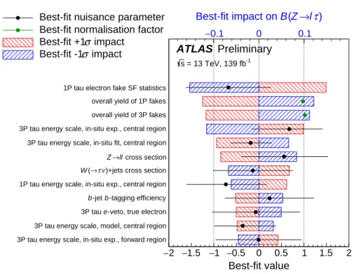
Systematic uncertainties are modelled by nuisance parameters (NP) with Gaussian constraints in the likelihood function. Impact of the uncertainties on both the shape and normalisation of the fitted distributions are taken into account. Uncertainties in the energy calibration and resolution, and the trigger, reconstruction, identification and isolation efficiencies of jets, electrons, muons, τ

and E

T

are considered. Theoretical uncertainties in the production cross sections affect only the predictions of simulated top, diboson, Higgs boson and W +jets events with a real τ

candidate, since the Z → ττ and signal yields are determined in the maximum-likelihood fit to data and the Z → `` yield is predicted with the measured value of σ(Z ) . Statistical uncertainties in the determination of the fake factors are also considered. They are modelled by one NP per bin that the fake factors are measured in. As noted in Section 4, the dominant uncertainties in the analysis are the systematics in the reconstructed τ

energy and the statistical ones in the determination of the fake yields.

For the µτ channel, the likelihood functions of the presented measurement and of the measurement in

Ref. [53] are combined. As the two measurements are statistically uncorrelated and the predictions are

based on different methods, nuisance parameters in the individual likelihood functions are considered

uncorrelated in the combination. The method of combination is the same as that in Ref. [13].

−0.1 0 0.1 τ)

→l Z ( B Best-fit impact on

3P tau energy scale, in-situ exp., forward region 3P tau energy scale, model, central region -veto, true electron e

3P tau

-tagging efficiency b

-jet b

1P tau energy scale, in-situ exp., central region )+jets cross section ν

τ

→ ( W

cross section

→ll Z

3P tau energy scale, in-situ fit, central region 3P tau energy scale, in-situ exp., central region overall yield of 3P fakes overall yield of 1P fakes 1P tau electron fake SF statistics

−2 −1.5 −1 −0.5 0 0.5 1 1.5 2 Best-fit value

Preliminary ATLAS

= 13 TeV, 139 fb-1

s

Best-fit nuisance parameter Best-fit normalisation factor

impact σ Best-fit +1

impact σ Best-fit -1

Figure 4: The best-fit values and uncertainties of nuisance parameters in the binned maximum-likelihood fit in theeτ channel. The parameters are ranked from top to bottom by their estimated impact on the signal branching ratio. Only the most highly ranked 12 parameters are shown.

−0.1 0 0.1

τ)

→l Z ( B Best-fit impact on

-bin) pT

-bin 4th track- pT

1P fake factor (2nd

τ τ

→ Z overall yield of 3P tau energy scale, in-situ exp., forward region

3P tau energy scale, model, central region 3P tau energy scale, in-situ fit, central region 1P tau energy scale, model, central region overall yield of 3P fakes 1P tau energy scale, in-situ exp., forward region 3P tau energy scale, in-situ exp., central region overall yield of 1P fakes 1P tau energy scale, in-situ fit, central region 1P tau energy scale, in-situ exp., central region

−2 −1.5 −1 −0.5 0 0.5 1 1.5 2 Best-fit value

Preliminary ATLAS

= 13 TeV, 139 fb-1

s

Best-fit nuisance parameter Best-fit normalisation factor

impact σ Best-fit +1

impact σ Best-fit -1

Figure 5: The best-fit values and uncertainties of nuisance parameters in the binned maximum-likelihood fit in theµτ channel. The parameters are ranked from top to bottom by their estimated impact on the signal branching ratio. Only the most highly ranked 12 parameters are shown.