τ τ DecayswiththeATLASDetector SearchfortheStandardModelHiggsBosoninHadronic Dissertation

Dissertation

Search for the Standard Model Higgs Boson in Hadronic τ ⁺ τ ⁻ Decays

with the ATLAS Detector

von

Daniele Zanzi

eingereicht an der

Fakult¨at f¨ur Physik

der

Technischen Universit¨at M¨unchen

erstellt am

Max–Planck–Institut f¨ur Physik (Werner–Heisenberg–Institut)

M¨ unchen

May 2014

Fakult¨at f¨ur Physik der Technischen Universit¨at M¨unchen

Max–Planck–Institut f¨ur Physik (Werner–Heisenberg–Institut)

Search for the Standard Model Higgs Boson in Hadronic τ ⁺ τ ⁻ Decays

with the ATLAS Detector Daniele Zanzi

Vollst¨andiger Abdruck der von der Fakult¨at f¨ ur Physik der Technischen Universit¨at M¨ unchen zur Erlangung des akademischen Grades eines

Doktors der Naturwissenschaften (Dr. rer. nat.) genehmigten Dissertation.

Vorsitzender: Univ.–Prof. Dr. A. Ibarra Pr¨ ufer der Dissertation:

1. Priv.–Doz. Dr. H. Kroha 2. Univ.–Prof. Dr. L. Oberauer

Die Dissertation wurde am 05.05.14 bei der Technischen Universit¨at M¨ unchen eingereicht

und durch die Fakult¨at f¨ ur Physik am ... angenommen.

Abstract

The discovery of a Higgs boson in di-boson decays, the evidence of its decays into fermion pairs and the compatibility of its measured properties with the Standard Model predictions support the electroweak symmetry breaking mechanism of the Standard Model.

The topic of this thesis is the search for the Higgs boson decays into a pair of τ leptons, important for probing the coupling of the Higgs boson to fermions. The search is performed in final states where both τ leptons decay hadronically using 4.6 fb

and 20.3 fb

of data collected by the ATLAS detector in proton-proton collisions at the Large Hadron Collider at center-of-mass energies of 7 and 8 TeV, respectively.

The signal selection is optimised for events with highly boosted Higgs bosons pro- duced via gluon fusion with additional jet or via vector boson fusion. In order to reduce systematic uncertainties, the major background contributions from Z → τ τ and multi-jet production processes have been measured using signal-free control data samples. The trig- ger and identification efficiencies of hadronically decaying τ leptons have been measured using dedicated calibration data samples.

An excess of events above the predicted background is found with observed (expected) significance of 2.3 σ (2.1 σ). The observation is compatible with the production of a Higgs boson with mass of 125 GeV and corresponds to a Higgs boson production cross section times branching ratio of µ = 1.2 ± 0.4(stat)

(syst) times the Standard Model prediction.

The Higgs boson mass determined from the observed invariant τ τ mass distribution is 125

GeV. The sensitivity of this analysis and its results are compatible with the ones obtained using a multivariate approach. The combination of searches for H → τ

τ

decays in fully leptonic and semi-leptonic and fully hadronic τ

τ

final states in √

s =

8 TeV data with multivariate analyses leads to a 4.1 σ evidence for Higgs boson decays

into τ lepton pairs.

Acknowledgements

This thesis has been written with the help of my thesis advisor Prof. Hubert Kroha and my supervisor Dr. Sandra Kortner at the Max-Planck-Institute for Physics in M¨ unchen.

During the three years of PhD I received great support from Prof. Stefania Xella and I

benefited from working in close collaboration with Dr. Soshi Tsuno.

Contents

Introduction 1

1 The Higgs boson of the Standard Model 3

1.1 The Standard Model and the EWSB . . . . 3

1.2 Indirect Constraints on the Higgs Boson Mass . . . . 5

1.3 Higgs Boson Production and Decay Modes . . . . 6

1.4 Direct Higgs Boson Searches . . . 12

1.5 Higgs Boson Discovery and Properties . . . 13

2 The Large Hadron Collider and the ATLAS Experiment 21 2.1 The Large Hadron Collider . . . 21

2.2 The ATLAS Detector . . . 23

2.2.1 The Detector Components . . . 24

2.2.2 The Trigger System . . . 28

2.2.3 The Luminosity Measurement . . . 28

2.2.4 The Reconstruction of Physics Object . . . 30

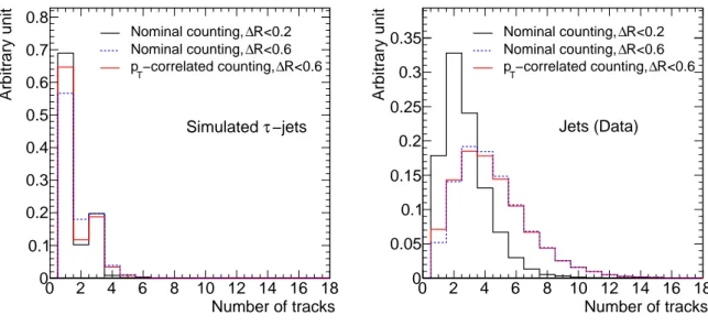
3 τ -jet Reconstruction and Trigger 33 3.1 Reconstruction of τ -jet Candidates . . . 34

3.1.1 The τ -jet Energy Calibration . . . 35

3.2 The τ-jet Identification . . . 37

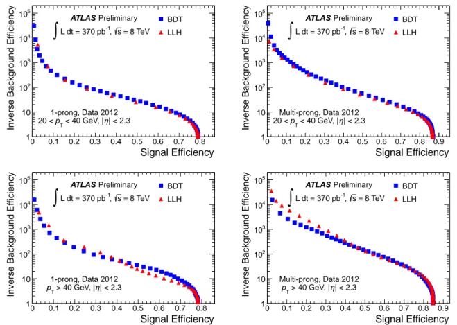
3.2.1 Measurement of the τ -jet Identification Efficiency . . . 38

3.3 The τ-jet Trigger . . . 45

3.3.1 Measurement of the τ -jet Trigger Efficiency . . . 47

3.4 τ-jet Trigger and Identification Efficiency for QCD jets . . . 48

4 H → τ

τ

Search in the Fully Hadronic Final State 51 4.1 Introduction . . . 51

4.2 Data and Simulated Samples . . . 54

4.2.1 Data . . . 54

4.2.2 Simulated Samples . . . 55

4.3 Selection of Physics Objects . . . 57

4.4 Event Selection and Categorisation . . . 59

4.4.1 Event Preselection . . . 59

4.4.2 Event Categorisation . . . 62

4.5 Invariant Mass Reconstruction . . . 71

i

4.6 Measurement of the Background Contributions . . . 76

4.6.1 Modelling of the Z → τ τ Background Process . . . 77

4.6.2 Modelling of the Multi-jet Background Process . . . 81

4.6.3 Validation of the Background Modelling . . . 83

4.7 Systematic Uncertainties . . . 84

4.7.1 Experimental Uncertainties . . . 86

4.7.2 Theoretical Uncertainties . . . 92

4.8 The Statistical Model . . . 95

4.9 Results . . . 101

4.9.1 Comparison with Results of Multivariate Analyses . . . 110

5 Conclusions 115

Bibliography 116

Appendices 129

A Validation of the Background Modelling 131

B m

Fit 143

Introduction

This thesis is about the search for the Higgs boson of the Standard Model of particle physics in its decay into a pair of hadronically decaying τ leptons with the ATLAS detector at the Large Hadron Collider (LHC) at CERN.

The Higgs boson is a consequence of electroweak symmetry breaking introduced in the Standard Model to give masses to the fundamental particles and to ensure the consistency of the Standard Model at high energies. While this theory has successfully passed many experimental tests, including the correct prediction of the W and Z boson masses, the last missing piece has been for a long time the direct detection of the Higgs boson. Finally in 2012, this particle has been discovered at the LHC in decays into pairs of electroweak vector bosons. All properties of the new particle are so far in agreement with the Standard Model predictions.

The search presented here is important because the Higgs boson decays into fermion pairs had not been discovered yet. These decays are required for the new particle to be also responsible for the generation of the fermion masses. Among the fermionic decays, the τ

τ

channel is the most sensitive for Higgs boson searches. It leads to three distinct final states depending on the decays of the τ lepton into leptons or hadrons.

The final states studied in this thesis contain two hadronically decaying τ leptons.

Compared to the other τ

τ

channels, the sensitivity of this final state depends on op- posing features. On the positive side, the signal acceptance profits from the large hadronic τ decay branching ratio and the relatively high τ

τ

invariant mass resolution, since there are only two neutrinos in the final state. On the negative side, this channel is harmed by the high rate of background of QCD jet production mimicking the hadronically decaying τ leptons. In order to suppress this background, the search is performed in events where the Higgs boson is produced together with two highly energetic jets emitted in the proton beam directions characteristic for vector boson fusion Higgs production or where the τ

τ

pair has high transverse momentum perpendicular to the beams characteristic for gluon fusion Higgs production in association with a recoiling jet.

Important for this search was the optimisation of the trigger and the measurement of the trigger and hadronic τ decay identification efficiencies.

The thesis is structured as follows. Chapter 1 introduces to the theoretical foundations for the analysis and summarises the status of the Higgs boson searches and measurements of its properties. Chapter 2 describes the LHC accelerator and the ATLAS detector.

Chapter 3 discusses the trigger and reconstruction algorithms for hadronically decaying τ leptons and the measurements of their performance. Chapter 4 describes the selection

1

of Standard Model H → τ

τ

decays in fully hadronic final states. The results are

summarised in Chapter 5.

Chapter 1

The Higgs boson of the Standard Model

1.1 The Standard Model and the EWSB

The Standard Model (SM) of particle physics [1–4] describes the known fundamental particles, fermions and bosons, and their interactions (see Fig. 1.1).

Except for the Higgs boson, which has spin zero, all bosons in the SM are vector fields with spin one which mediate the fundamental interactions between the spin 1/2 fermions.

The massless photon and the massless gluons mediate the electromagnetic and the strong force, respectively, while the massive W

and Z bosons mediate the weak interaction.

The only scalar boson predicted by the SM, the Higgs boson, has recently been dis- covered in its decays into photon or weak boson pairs [5, 6]. The search for it in decays into τ lepton pairs is the topic of this thesis.

The interactions of the SM are described by a local SU (3) × SU(2)

× U (1)

gauge symmetry. The non-Abelian SU (3) gauge symmetry determines the strong interaction between quarks and eight massless gluons, while the SU(2)

× U (1)

gauge symmetry governs the electroweak interaction mediated by the photon and the W

and Z bosons.

The local gauge theories predict massless intermediate vector bosons. The global SU (2) symmetry, together with parity violation, prohibits fermion masses.

In the SM, the masses of the fundamental fermions and bosons are generated by spon- taneous breaking of the electroweak SU (2)

× U (1)

gauge symmetry via the introduction of a scalar SU(2)

doublet field, the Higgs field, with a ground state invariant only under the electromagnetic U (1)

and the strong SU (3) gauge symmetry.

The problem that at first prevented the application of spontaneous symmetry breaking (SSB) in particle physics is the Goldstone theorem [7]. This theorem states that if in a relativistic quantum field theory, like the SM, the field equations are covariant under a continuous symmetry, then either the ground state is invariant under the same symmetry or there must exist scalar particles with zero mass, the Goldstone bosons, corresponding to the broken symmetry generators. Since such scalar massless particles have not been observed, SSB in the SM seemed to violate the Goldstone theorem.

The solution first suggested by Anderson [8] based on similar effects occurring in su-

3

1/2 2/3 2.3 MeV

u

up 1/2 -1/3

4.8 MeV

d

down

1/2 1

0.511 MeV

e

electron

1/2 0

0

ν

1/2 2/3 1.27 GeV

c

charm 1/2 -1/3

95 MeV

s

strange

1/2 1

105 MeV

µ

muon

1/2 0

0

ν

1/2 2/3 173 GeV

t

top 1/2 -1/3

4 GeV

b

bottom

1/2 1

1.777 GeV

τ

tau

1/2 0

0

ν

1 0

0

γ

photon

1 0

0

g

gluon

1 0

91.2 GeV

Z

1 ±1

80.4 GeV

W

0 0

126 GeV

H

Higgs

Q u ar ks L ep to n s

Bosons

I II III

SpinCharge Mass

Symbol Name

Families

Figure 1.1: Overview of the fundamental particles of the SM. For each particle, its mass,

spin and electric charge quantum number are indicated. Fermions, spin 1/2 particles, are

arranged in three families, with a pair of leptons (violet) and a pair of quarks (orange)

and the same quantum numbers, but different masses. Bosons (green) include the vector

bosons mediating the fundamental interactions and the scalar Higgs boson. The massless

photon mediates the electromagnetic force between all particles with electric charge. The

eight massless gluons mediate the strong interaction between quarks and gluons. The

massive W

and Z bosons mediate the weak interaction. The massive scalar Higgs boson

couples to all massive particles. For each fermion there is an anti-fermion, a particle with

the same mass, but opposite charges. For the electrically neutral neutrinos it is not yet

known whether they are different from their anti-particles.

1.2 Indirect Constraints on the Higgs Boson Mass 5

perconductors is that the mechanisms of giving masses to gauge bosons and of preventing the appearance of massless scalar particles are related. In 1964/65 this idea has been applied to particle physics by Brout and Englert [9], Higgs [10, 11] and Kibble, Guralnik and Hagen [12] in what is now known as the Brout-Englert-Higgs (BEH) mechanism.

They proposed that in relativistic gauge theories the massless Goldstone bosons can be translated into the longitudinal polarisation states of massive gauge bosons. In 1967, Weinberg [2] and Salam [3] applied the BEH mechanism to the SU(2)

× U (1)

gauge theory of the electroweak interaction introduced by Glashow [1].

In the SU (2)

× U (1)

gauge theory, the Higgs field is a complex scalar weak isospin doublet with hypercharge Y = +1 and no electric charge. A non-vanishing vacuum expectation value v = h φ i

/ √

2 of the Higgs field φ spontaneously breaks the electroweak gauge symmetry to the remaining electromagnetic (EM) gauge symmetry U (1)

giving masses to the W

and Z bosons while leaving the photon massless.

Via the SU (2)

gauge symmetry, the three massless Goldstone boson excitations of the symmetry breaking ground state are transformed into the longitudinal polarisation states of the massive W

and Z fields. The fourth excitation of the ground state is the massive scalar Higgs boson. Its couplings to the weak bosons are proportional to the square of the weak boson masses which are predicted to be m

=

vg and m

=

v p

g

+ g

, where g and g

are the SU(2)

and U (1)

gauge coupling constants, respectively.

The BEH mechanism also generates fermion masses via the introduction of Yukawa- type interactions between the fermions and the Higgs field with coupling constants g

=

√ 2m

/v proportional to the fermion masses. The test of the existence of such Yukawa couplings of the SM fermions to the Higgs field is subject of this thesis.

The Higgs boson mass m

and the fermion masses are not predicted by the SM.

1.2 Indirect Constraints on the Higgs Boson Mass

Upper and lower bounds on the Higgs boson mass follow from consistency requirements in the SM. An upper bound is introduced by the requirement of unitarity [13–16], for instance for the amplitude of longitudinal W scattering W

W

→ W

W

, which would grow proportionally to the center-of-mass energy of the scattering, eventually violating unitarity, if there is no contribution from the exchange of a virtual Higgs boson with m

. 800 GeV or new physics beyond the SM at the TeV scale. For this reason, direct SM Higgs boson searches have been devised to explore the mass range up to 1 TeV.

Other theoretical arguments concerning the finiteness of the Higgs self-coupling λ un- der radiative corrections and the stability of the Higgs ground state [17–21] lead to even more stringent upper and lower bounds. Quantum effects of Higgs boson loops lead to a divergence of λ at high energies if the Higgs boson is heavier than about 160 GeV [22]. If the Higgs boson is too light, quantum corrections from top quark loops drive λ to negative values making the SM vacuum unstable. To ensure vacuum stability, the Higgs boson has to be heavier than 129.4 ± 1.8 GeV [23].

Indirect constraints on the Higgs boson mass can be derived from the precision mea-

surements of electroweak observables which depend logarithmically on m

via virtual

Higgs boson radiations. The constraint on the Higgs boson mass from the combined elec- troweak precision measurements at LEP, SLC, Tevatron and LHC is m

= 94

GeV [24]

as shown in Fig. 1.2 which is in agreement with the direct measurements of the Higgs boson mass performed by the ATLAS and CMS experiments [5, 6] within 1.3 σ.

[GeV]

M

60 70 80 90 100 110 120 130 140

2

χ∆

0 0.5 1 1.5 2 2.5 3 3.5 4 4.5 5

σ 1

σ 2 SM fit

measurement SM fit w/o MH

ATLAS measurement [arXiv:1207.7214]

CMS measurement [arXiv:1207.7235]

G fitter

Sep 12

Figure 1.2: ∆χ

of the global fit to the electroweak precision measurements as a function of the Higgs boson mass [24]. The data points show the direct measurements of m

by the ATLAS and CMS experiments.

1.3 Higgs Boson Production and Decay Modes

The SM Higgs boson couplings to fermions, proportional to the fermion masses, and to the weak vector bosons, proportional to the square of the vector boson masses, as well as the Higgs boson self-coupling are illustrated in Table 1.1 [25]. The dominant couplings are to the top quark and to the W and Z bosons.

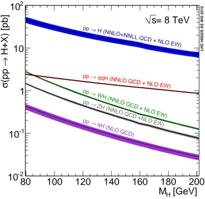
The main Higgs boson production processes at hadron colliders are gluon fusion (ggF), the vector boson fusion (VBF), associated production with a vector boson (VH) and the associated production with a top quark pair (t ¯ tH) as illustrated in Table 1.2. Fig. 1.3 shows the cross sections of these processes in pp collisions as a function of the Higgs boson mass at a center-of-mass energy of 8 TeV [26].

Gluon fusion is the dominant Higgs production process at the LHC with the main contribution from the top quark loop. The cross section depends on the distribution function (PDF) of the gluon momentum fraction in the proton and on QCD radiative corrections. The QCD corrections have been computed in NLO perturbation theory [28,29] with NNLO contributions calculated in the large-m

approximation

[30–37] which is expected to deviate from the complete result by less than 1% for m

≤ 300 GeV [38–43].

1

In the large-m

approximation, the gg → H loop is described by an effective point interaction between

1.3 Higgs Boson Production and Decay Modes 7

Table 1.1: SM Higgs boson couplings [25].

Yukawa coupling to fermions

H f

f ¯ g

= √

2

Couplings to weak vector bosons (V = W, Z)

H V

V g

=

g

=

H H

V V g

=

g

=

Higgs self-coupling

H H

H g

=

H H

H

H

g

=

Table 1.2: SM Higgs boson production modes at the LHC. The predicted cross sections for m

= 125 GeV at √

s = 8 TeV [26,27], calculated to the higher orders in perturbation theory as indicated, are given.

Production LO diagram Cross section [pb] Order in

process perturbation theory

ggF g

g

t H

19.52

NNLO+NNLL QCD, NLO EW

VBF q

q

V V

H

1.578

NLO QCD+EW, approx. NNLO QCD

VH q

¯

q V

H WH: 0.697

ZH: 0.394

NNLO QCD, NLO EW

t ¯ tH g

g

H t

¯ t t

¯ t

0.130

^{NLO QCD}

1.3 Higgs Boson Production and Decay Modes 9

[GeV]

M

80 100 120 140 160 180 200

H+X) [pb] → (pp σ

10

10

1 10 10

= 8 TeV s

LHC HIGGS XS WG 2012

H (NNLO+NNLL QCD + NLO EW)

→ pp

qqH (NNLO QCD + NLO EW)

→ pp

WH (NNLO QCD + NLO EW) pp →

ZH (NNLO QCD +NLO EW) pp →

ttH (NLO QCD) pp →

Figure 1.3: SM Higgs boson production cross sections in pp collisions at √

s = 8 TeV as a function of the Higgs boson mass [26]. The bands represents the theoretical uncertainties.

It is necessary to take into account higher-order QCD corrections in the ggF cross section prediction because of the slow convergence of the perturbative expansion in α

. The LO cross section is increased by 80-100% at NLO and by an additional 25% at NNLO.

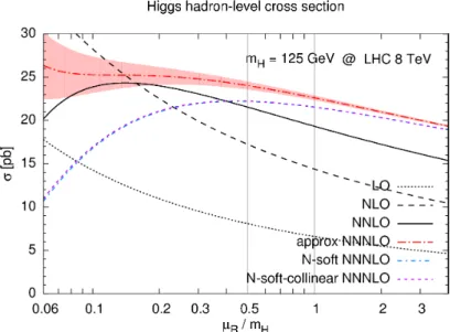
Fig. 1.4 shows the SM Higgs boson production cross section for ggF in different orders of perturbation theory as a function of the renormalisation scale µ

[44]. The large NLO and NNLO corrections are related to the large scale dependence of the LO and NLO cross sections. A moderate scale dependence is reached only at NNLO suggesting that the size of the N

LO corrections should be smaller. However, approximated N

LO calculations [44, 45] indicate that the cross section may still increase by as much as 17% [44].

Other sizeable corrections are due to soft-gluon radiation computed in NNLL approx- imation [46], and to EW corrections computed at NLO [47–51].

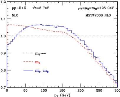
Because of the large contribution of higher order QCD processes to the production cross section, many Higgs boson searches, including the one presented in this thesis, take into account the production of one or two additional jets. In such events, the Higgs boson recoils against the jet(s) acquiring significant momentum. The high transverse momentum p

of the Higgs boson in higher order ggF production provides strong discrimination between signal and background. The p

dependence of the cross section has been com- puted at NNLL+NNLO for the correct top and bottom quark masses [52]. Heavy quark mass effects are important for the differential ggF cross section as a function of p

although the total cross section is little affected. Fig. 1.5 shows the impact of the top and bottom quark loop contributions on the Higgs boson transverse momentum spectrum at

the gluons and the Higgs boson and contributions from W boson and b quark loops are neglected.

0 5 10 15 20 25 30

0.06 0.1 0.2 0.3 0.5 1 2 3

σ [pb]

µ_F / m_H

Higgs hadron-level cross section

m_H = 125 GeV @ LHC 8 TeV

LO NLO gg NLO NNLO gg NNLO 0

5 10 15 20 25 30

0.06 0.1 0.2 0.3 0.5 1 2 3

σ [pb]

µ_R / m_H

Higgs hadron-level cross section

m_H = 125 GeV @ LHC 8 TeV

LO NLO gg NLO NNLO gg NNLO

Figure 1.4: Gluon fusion production cross section of the SM Higgs boson with m

= 125 GeV at √

s = 8 TeV as a function of the renormalisation scale µ

in different orders of perturbation theory [44].

NLO compared to the large-m

approximation. The bottom quark contribution is impor- tant in the low-p

region, while at high-p

the top quark contribution has a significant impact and the large-m

approximation becomes invalid. The correct description of the Higgs boson transverse momentum distribution is important for the analysis presented here because the high momentum Higgs boson production in ggF is used in the event selection.

VBF production, even though it has an order of magnitude smaller cross section than ggF production, is very important for discriminating signal from background in pp collisions due to its characteristic final state. The two quarks in the initial state in this case each radiate vector bosons which annihilate with each other producing the Higgs boson.

In the final state, the two quarks hadronize into two jets emitted in the forward regions of the detector close to the proton beams while the Higgs boson decays in the central part of the detector. Hadronic emission around the Higgs boson is suppressed due to the fact that the two quarks are not connected by colour fields and the hadron production, therefore, mostly develops along the quark directions. This provides an additional signature for the VBF event selection, which can hardly be imitated by other SM processes.

VBF at LO is an electroweak process. QCD corrections are only on the order of 5%.

The cross section has been computed with full NLO QCD and EW corrections [53, 54]

and approximate NNLO QCD corrections [55].

The ggF and VBF processes are complementary for the test of the SM because ggF is

determined by the Higgs Yukawa couplings to fermions while VBF depends on the Higgs

boson couplings to the weak vector bosons. It is, therefore, important to explore both

production processes in order to test the role of the Higgs field in the SM.

1.3 Higgs Boson Production and Decay Modes 11

Figure 1.5: Transverse momentum distribution of the SM Higgs boson with m

= 125 GeV at NLO in the large-m

approximation (dotted black line), for the exact top quark loop contribution (red dashed line) and with both top and bottom quark loop contributions (solid blue line) [52].

The cross section for Higgs boson production in association with a weak vector boson, also known as Higgs-strahlung, has been computed including NNLO QCD [56, 57] and NLO EW corrections [58]. The production in association with a t ¯ t pair has the smallest cross section, but is relevant because it allows for the direct measurement of the top quark Yukawa coupling. Only NLO QCD corrections have been calculated so far [59–62].

The branching ratios (BR) of the Higgs boson decays into different final states are determined by the couplings of the Higgs boson to the final state particles. As shown in Fig. 1.6 [27], the SM Higgs boson mainly decays into two weak vector bosons for m

above the threshold. For m

below about 140 GeV, these decay modes are suppressed since only one of the two bosons can be produced on-shell.

In the low-mass region around the measured Higgs boson mass of 125 GeV, the main decay mode is into b ¯ b pairs because b quarks are the heaviest particles which can be pair- produced on-shell in Higgs decays. The next largest BR into fermions is for decays into τ

τ

. Decays into c¯ c are very difficult to distinguish from QCD di-jet events. Decays into µ

µ

have a very small BR, but provide high µ

µ

invariant mass resolution.

The observable bosonic decay modes in the low-mass region are H → W W

, ZZ

and γγ. BR(H → W W

) is larger than the BR(H → ZZ

) because of the twice larger

number of degrees of freedom compared to Z and because of the smaller W mass and,

therefore, the larger phase space for the decay. BR(H → γγ) is very small because the

decay occurs only in second order perturbation theory through W boson and top quark

loops. However, this decay mode is important for Higgs boson searches due to the clear

signature of two highly energetic photons and the high γγ invariant mass resolution. The

[GeV]

M

90 200 300 400 1000

H ig g s B R + T o ta l U n c e rt [ % ]

10-4

10-3

10-2

10-1

1

LHC HIGGS XS WG 2013

b b τ τ

µ µ c c

t t gg

γ γ Zγ

WW

ZZ

[GeV]

M

80 100 120 140 160 180 200

H ig g s B R + T o ta l U n c e rt [ % ]

10-4

10-3

10-2

10-1

1

LHC HIGGS XS WG 2013

b b τ

τ

µ µ c c

gg

γ

γ Zγ

WW

ZZ

Figure 1.6: SM Higgs boson decay branching ratios as a function of the Higgs boson mass in the whole range up to 1 TeV allowed for consistency of the SM (left) and in the low mass range (right) [27]. The bands represent the theoretical uncertainties.

H → gg decay mode cannot be exploited due to the large QCD di-jet background.

1.4 Direct Higgs Boson Searches

A lower bound on the Higgs boson mass of 114.4 GeV at 95% CL has been obtained before LHC at the Large Electron-Positron collider (LEP) at CERN at center-of-mass energies of up to √

s = 209 GeV [63].

At the Tevatron, the proton-antiproton collider at the Fermi National Accelerator Laboratory, direct Higgs boson searches have been carried out at a center-of-mass energy of √ s = 1.96 TeV in the mass range of 90 . m

. 200 GeV. In 2013, an excess of events around m

= 125 GeV mainly from searches in the V H → V b ¯ b channel has been found with a significance of 3.1 σ [64].

The direct searches carried out at the LHC are based on data collected in 2011 at

√ s = 7 TeV and in 2012 at √

s = 8 TeV corresponding to integrated luminosities of about 5 fb

and 20 fb

, respectively. The search programme covered the mass range from the LEP lower mass limit up to about 1 TeV [65]. In the low mass range, despite the small branching ratios, the channels with highest sensitivity for the Higgs boson search are Higgs boson decays into a pair of vector bosons, namely H → γγ, H → ZZ

→ l

l

l

l

(H → 4l) and H → W W

→ lνl

ν. The other two decay channels accessible in the low- mass range, but with lower sensitivity, are the fermionic decays H → τ

τ

and H → b ¯ b.

In the high mass range, the most sensitive channels are H → W W → lνl

ν, lνqq

and

H → ZZ → l

l

l

l

, l

l

q q. ¯

1.5 Higgs Boson Discovery and Properties 13

1.5 Higgs Boson Discovery and Properties

The discovery of a new particle compatible with the SM Higgs boson has been pub- lished by both ATLAS and CMS on July 4

, 2012 [5, 6]. The discovery is based on integrated luminosities of 4.8 − 5.1 fb

at √

s = 7 TeV and 5.8 − 5.3 fb

at √

s = 8 TeV.

The most sensitive channels in both experiments are H → 4l, H → γγ and H → W W

→ eνµν. The significance of the excess of events observed around m

= 125 GeV is above 5 σ. Since then, the discovery has been confirmed in the di-boson final states with in- creased precision including all data collected in 2012. In November 2013, also evidence for Higgs boson decays into fermions has been found with more than 3 σ significance in the H → τ

τ

and H → b ¯ b channels by both experiments compatible with the SM Higgs boson at m

= 125 GeV [66–68]. The search presented here contributes to the result in the τ

τ

channel.

Using the di-boson decay channels, the properties of the new particle, production and decay rates, mass, couplings to other SM particles and spin and CP quantum numbers have been measured. The results of the two experiments ATLAS and CMS [69–72] are compatible. Here, only the results published by the ATLAS collaboration are discussed.

100 110 120 130 140 150 160

Events / 2 GeV

2000 4000 6000 8000 10000

γ γ

→ H

Ldt = 4.8 fb-1

∫

= 7 TeV s

Ldt = 20.7 fb-1

∫

= 8 TeV s

ATLAS

Data 2011+2012

=126.8 GeV (fit) SM Higgs boson mH

Bkg (4th order polynomial)

[GeV]

γ

mγ

100 110 120 130 140 150 160

Events - Fitted bkg

-200 -100 0 100 200 300 400 500

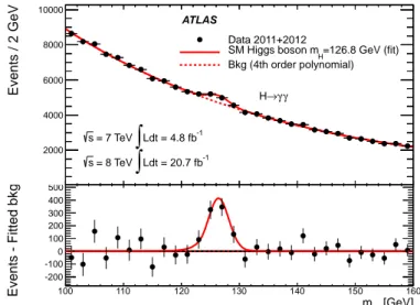
Figure 1.7: Invariant mass distribution of di-photon candidates in the ATLAS inclusive H → γγ search. The fit of a SM Higgs boson signal (with m

= 126.8 GeV) on top of a smooth background parametrisation is superimposed on the data points. The bottom panel shows the residual distribution of data with respect to the fitted background [71].

Figs. 1.7-1.9 show the mass distributions used for the evaluation of the signals in the

H → γγ, H → 4l and H → W W

→ lνl

ν channels, respectively, for the full 7 and

8 TeV data sets [71]. Signals with significances of 7.4, 6.6 and 3.8 standard deviations,

respectively, have been found.

[GeV]

m

100 150 200 250

Events/5 GeV

0 5 10 15 20 25 30 35 40

Ldt = 4.6 fb

∫

= 7 TeV s

Ldt = 20.7 fb

∫

= 8 TeV s

→ 4l

→ ZZ*

H

Data 2011+ 2012 SM Higgs Boson

=124.3 GeV (fit) mH

Background Z, ZZ*

t Background Z+jets, t Syst.Unc.

ATLAS

Figure 1.8: Four-lepton invariant mass distribution of data events passing the H → 4l selection together with the estimated background contributions and the fitted SM Higgs boson signal at m

= 124.3 GeV [71].

The Higgs boson mass measurement is performed using the final states with high mass resolution, H → γγ and H → 4l [71]. The mass resolution in the H → γγ channel [73]

is 1.4 − 2.5 GeV at m

= 126.5 GeV, depending on the event selection category. The precision of the measurement is limited by the photon energy scale uncertainty. In the H → 4l [74] channel a mass resolution of 1.6 − 2.4 GeV is achieved at m

= 125 GeV depending on the lepton flavours. The uncertainty in the measurement is dominated by statistics. The measured mass value is 126.8 ± 0.2(stat) ± 0.7(syst) GeV in the H → γγ channel and 123.4

(stat)

(syst) GeV in the H → 4l channel. The two measurements agree within 2.4 σ. The combined value is

m

= 125.5 ± 0.2(stat)

(syst) GeV.

The Higgs boson production cross sections times branching ratios have been measured in the di-boson final states H → γγ, H → 4l and H → W W

→ lνl

ν and in the fermionic channels H → τ

τ

and H → b ¯ b. Combining all channels the signal strength, the ratio of the measured signal yield to the one predicted by the SM, for m

= 125.5 GeV is

µ = σ/σ

= 1.30

compatible with the SM prediction within 11% [75]. The signal strengths measured in

the individual channels are summarised in Fig. 1.10.

1.5 Higgs Boson Discovery and Properties 15

60 80 100 120 140 160 180 200 220 240 260

Events / 10 GeV

100 200 300 400 500 600 700

800 Data 2011+2012

Total sig.+bkg.

SM Higgs boson = 125 GeV mH

WW t t Other VV Single Top W+jets

γ* Z/

ATLAS

Ldt = 4.6 fb-1

∫

= 7 TeV s

Ldt = 20.7 fb-1

∫

= 8 TeV s

+ 0/1 jets ν νl

→l

→WW*

H

[GeV]

mT

60 80 100 120 140 160 180 200 220 240 260

Data - Bkg.

-20 0 20 40 60 80

100 Bkg. subtracted data

= 125 GeV

H

SM Higgs boson m

[GeV]

m

50 100 150 200 250 300

Events / 20 GeV

0 2 4 6 8 10 12

Data 2011+2012 Total sig.+bkg.

= 125 GeV VBF mH

= 125 GeV ggF mH

t t WW

γ* Z/

Other VV Single Top W+jets

ATLAS

Ldt = 4.6 fb-1

∫

= 7 TeV s

Ldt = 20.7 fb-1

∫

= 8 TeV s

≥ 2 j ν + µ ν

→e

→WW*

H

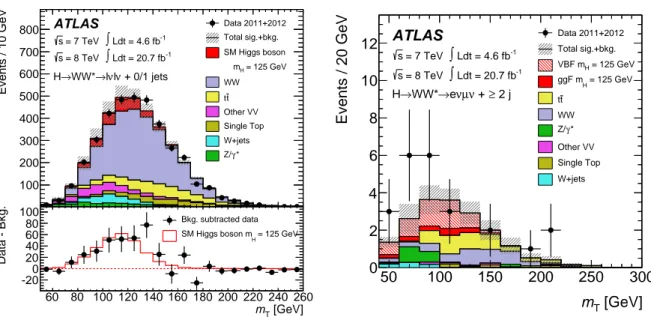
Figure 1.9: Transverse mass distributions of events after the H → W W

→ lνl

ν selection

with N

≤ 1 (left) and N

≥ 2 (right) additional jets. The signal is stacked on top of

the background contributions. In the right plot, VBF and ggF production contributions

are shown separately. The hatched area shows the total uncertainty on the signal and

background yields. The lower panel in the left plot shows the residual distribution of the

data with respect to the estimated background in comparison with the m

distribution

expected for a SM Higgs boson with m

= 125 GeV [71].

µ ) Signal strength (

-0.5 0 0.5 1 1.5 2

ATLAS Prelim.

Ldt = 4.6-4.8 fb

∫

= 7 TeV s

Ldt = 20.3 fb

∫

= 8 TeV s

= 125.5 GeV m H

0.28 -

0.33

= 1.57

µ γ γ

→ H

0.12 -

0.17 +

0.18 -

0.24 +

0.22 -

0.23 +

0.35 -

0.40

= 1.44

µ

→ 4l ZZ*

→ H

0.10 -

0.17 +

0.13 -

0.20 +

0.32 -

0.35 +

0.29 -

0.32

= 1.00

µ → l ν l ν WW*

→ H

0.08 -

0.16 +

0.19 -

0.24 +

0.21 -

0.21 +

0.20 -

0.21

= 1.35

, ZZ*, WW* µ

γ γ

→ H

Combined

0.11 -

0.13 +

0.14 -

0.16 +

0.14 -

0.14 +

0.6 -

0.7

= 0.2

µ b

→ b W,Z H

<0.1

±0.4

±0.5

0.4 -

0.5

= 1.4

µ

(8 TeV data only)

τ τ

→ H

0.1 -

0.2 +

0.3 -

0.4 +

0.3 -

0.3 +

0.32 -

0.36

= 1.09

τ µ τ , b

→ b H

Combined

0.04 -

0.08 +

0.21 -

0.27 +

0.24 -

0.24 +

0.17 -

0.18

= 1.30

µ

Combined

0.08 -

0.10 +

0.11 -

0.14 +

0.12 -

0.12 +

Total uncertainty µ

σ on

± 1

(stat.) σ

theory )

sys inc.

(

σ

(theory) σ

Figure 1.10: Measured signal strengths for different decay channels of the Higgs boson

with mass m

= 125.5 GeV [66, 67, 71] (updates in Ref. [75]).

1.5 Higgs Boson Discovery and Properties 17

The signal strengths µ for different production and decay modes are shown in Fig.

1.11. The vector boson mediated production processes VBF and VH are distinguished from the fermion mediated processes ggF and t ¯ tH. Since the branching ratio scale factors B/B

can be different for the different channels, the contours in the µ

vs. µ

plane cannot be directly compared. Only the ratios µ

× B/B

/µ

× B/B

for the different channels can be compared and show good agreement among each other and with the SM expectation of unity. A 4.1 σ evidence for VBF Higgs boson production

τ τ ,ZZ*,WW*, γ

γ ggF+ttH

µ

-2 -1 0 1 2 3 4 5 6

ττ,ZZ*,WW*,γγ VBF+VH

µ

-2 0 2 4 6 8

10

Best fit 68% CL 95% CL

γ γ

→ H

→ 4l ZZ*

→ H

ν νl

→ l WW*

→ H

τ τ

→ H

Preliminary ATLAS

Ldt = 4.6-4.8 fb

∫

= 7 TeV s

Ldt = 20.3 fb

∫

= 8 TeV s

= 125.5 GeV mH

Figure 1.11: 68% and 95% CL contours of the VBF and VH vs. ggF and ttH production strengths of the Higgs boson measured in the H → γγ, H → ZZ

→ 4l, H → W W

→ lνl

ν and H → τ

τ

channels for a Higgs boson mass of 125.5 GeV [75].

is found from the measurement of [75]

µ

/µ

= 1.4

(stat)

(syst).

The Higgs boson coupling strengths have been determined from combined fits to the

measurements of the signal strengths µ

= σ

BR

/σ

BR

with σ

BR

= Γ

Γ

/Γ

and

the partial and total widths Γ

and Γ

of the Higgs boson in the H → γγ , H → 4l,

H → W W

→ lνl

ν, H → b ¯ b and H → τ

τ

channels. Based on the assumption that

the signals observed in the different final states originate from the same narrow resonance

with m

= 125.5 GeV, the partial widths Γ

and, therefore, the squares of the couplings

y

for the production and decay modes are measured relative to the SM LO predictions

κ

= y

/y

= Γ

/Γ

, where i = W, Z, t, b, τ . The κ

and κ

scale factors for the loop

processes H → γγ and gg → H, respectively, are functions of the other coupling scale factors as predicted by the SM.

To test the couplings to fermions and vector bosons, universal coupling scale factors κ

= y

/y

and κ

= y

/y

as in the SM are assumed for the weak gauge bosons and for the fermions, respectively. As shown in Fig. 1.12 [75], the results for the individual decay channels and their combination are in good agreement with the SM expectation.

Among the channels considered only the H → γγ decay is sensitive to the relative sign of κ

and κ

via the interference of W boson and top quark loops.

Figure 1.12: 68% CL contours of the universal scale factors κ

and κ

of the couplings of the Higgs boson to weak gauge bosons and fermions in the SM [75].

For the test of the spin and parity quantum numbers of the Higgs boson, the SM hypothesis J

= 0

has been compared to the alternative hypotheses 0

, 1

, 1

and 2

in fits to distributions of kinematical variables of the di-boson final states [72, 76]. Fig.

1.13 summarises the tests of the spin-parity hypotheses. In all cases, the SM J

= 0

quantum numbers are favoured while the 0

, 1

, 1

and 2

hypotheses are rejected at 97.8%, 99.97%, 99.7% and > 99.9% CL

, respectively.

The measurements of the couplings, the spin and the parity of the new particle strongly

support the hypothesis that it is the SM Higgs boson. It still needs to be investigated

however whether the Higgs boson properties show effects of physics beyond the SM.

1.5 Higgs Boson Discovery and Properties 19

= 0

J

J

= 1

J

= 1

J

= 2

ATLAS

→ 4l ZZ*

→ H

Ldt = 4.6 fb-1

∫

= 7 TeV s

Ldt = 20.7 fb-1

∫

= 8 TeV s

γ γ

→ H

Ldt = 20.7 fb-1

∫

= 8 TeV s

ν ν e µ ν / µ ν

→ e WW*

→ H

Ldt = 20.7 fb-1

∫

= 8 TeV s

σ 1

σ 2

σ 3

σ 4

Data

expected CL

= 0

assuming J

± 1

)

( J

CL

10

10

10

10

10

10

1

Figure 1.13: Expected (full blue triangles) and observed (full black circles) CL

confidence

levels for the rejection of alternative spin-parity hypotheses for the Higgs boson with

respect to the SM J

= 0

hypothesis [72]. CL

is a modified confidence level to account

for possible downward fluctuations of the background estimate.

Chapter 2

The Large Hadron Collider and the ATLAS Experiment

The Large Hadron Collider (LHC) started operation end of 2009 and since then de- livered more than 25 fb

of data at the highest center-of-mass energies to the ATLAS and CMS experiments for the search for the Higgs boson and new physics beyond the Standard Model.

This chapter is devoted to an overview of the LHC (Section 2.1) and of the ATLAS detector (Section 2.2), with which the data analysed in this thesis have been recorded.

2.1 The Large Hadron Collider

The Large Hadron Collider (LHC) at CERN (Geneva, Switzerland) [77] is a proton storage ring of 27 km circumference in the tunnel of the LEP accelerator designed to provide colliding proton beams for a wide physics programme which includes the search for the Higgs boson and the measurement of its properties as well as the exploration of the TeV energy scale in the search for physics beyond the SM. The LHC has been designed for a center-of-mass energy of √

s = 14 TeV and a maximum instantaneous luminosity of L = 10

cm

s

. The proton beams are kept in their orbit by superconducting dipole magnets providing a magnetic field of up to 8 T.

In 2012, two years after the start of operations, the LHC collided protons at the record center-of-mass energy of √

s = 8 TeV and already reached almost the design luminosity (see Table 2.1 for details).

The acceleration of protons to such high energies is achieved by a complex chain of accelerators, as sketched in Fig. 2.1, where the energy and intensity of the beams is increased in steps. In the first step, the linear accelerator LINAC 2 accelerates the protons to 50 MeV, followed by then three synchrotrons, the Booster, the Proton Synchrotron (PS) and the Super Proton Synchrotron (SPS), which store the protons and accelerate them to 1.4, 25 and 450 GeV, respectively. In these rings, the proton beams are bunches to provide stable beams and collisions with high luminosity. Once the protons have been injected into the LHC, their energies are ramped up to the collision energy where they are collided. One fill of the LHC lasts for several hours, until the beam intensity has degraded too much and the beams are dumped on a dedicated target.

21

Table 2.1: Parameters of the pp collisions delivered by LHC in 2011 and 2012. The average number of interactions per bunch crossing is given by the mean of the Poisson distribution of the number of inelastic interactions per bunch crossing µ = L σ

/n

f

, where L is the luminosity, σ

the pp inelastic cross section (71.5 mb at 7 TeV and 73.0 mb at 8 TeV), n

the number of bunches and f

the proton revolution frequency [78].

Parameter 2011 2012

√ s [TeV] 7 8

Number of colliding bunches 1380 1380

Bunch spacing [ns] 50 50

Maximum bunch intensity [protons/bunch] 1.45 × 10

1.7 × 10

Peak luminosity [cm

s

] 3.7 × 10

7.7 × 10

Maximum average number of interactions per

bunch crossing 32 70

Longest beam lifetime [hours] 26 23

2.2 The ATLAS Detector 23

Figure 2.1: Sketch of the LHC accelerator and storage rings ( c CERN).

2.2 The ATLAS Detector

ATLAS [79] is one of the four experiments installed along the LHC ring and, like CMS [80], is designed as a multi-purpose detector to test the SM and search for new physics at the TeV scale. The other two experiments are ALICE [81], which is specialised in heavy ion physics, and LHCb [82], which focuses on B-meson physics.

ATLAS is designed to reconstruct and identify a wide range of signatures, like missing transverse momentum E

, secondary vertices and high-p

leptons and jets. The guiding principles of the detector design are as follows:

⊲ Good momentum resolution and high reconstruction efficiency of the tracking sys- tem.

⊲ Accurate electromagnetic and hadronic energy measurements in the calorimeters for the reconstruction and identification of muons, electrons, photons, jets, hadronic τ decays and E

.

⊲ High granularity and solid angle coverage.

⊲ Efficient reconstruction of secondary vertices.

⊲ Radiation-hard detectors and front-end electronics.

Figure 2.2 shows a schematic view of the ATLAS detector. It consists of a high precision

silicon tracking detector surrounded by a straw tube tracker in a 2 T solenoidal magnetic

field. The superconducting magnet coil is surrounded by the electromagnetic and hadronic

calorimeters. The outer-most part of the detector, defining its size of 44 m in length and

more than 25 m in height, is the muon spectrometer with its own air-core toroidal magnetic field. The precision muon tracking and trigger detectors are installed on the eight toroidal coils in the barrel and on three wheels in the two endcap regions.

Figure 2.2: Schematic overview of the ATLAS detector (ATLAS Experiment c CERN).

In the ATLAS coordinate system [79] the z axis points along the beam direction, the y axis upwards and the x axis towards the center of the LHC ring. Paths of particles crossing the ATLAS detector are usually described in polar coordinates with the azimuthal angle φ between − π and π and φ = 0 on the positive x axis and with the polar angle θ between 0 and π and θ = 0 on the positive z axis. Instead of the polar angle frequently the pseudo-rapidity η = − ln tan(θ/2) is used, which equals the Lorentz invariant rapidity y =

ln

E+pz

E−pz

in the limit of massless particles, where p

is the momentum component along the beam axis. Angular separations between particle tracks are usually measured by the distance ∆R = p

(∆φ)

+ (∆η)

in the η − φ plane.

2.2.1 The Detector Components

At the center of the ATLAS detector is the Inner Detector (ID) shown in Fig. 2.3.

It is composed of the silicon pixel and silicon microstrip trackers (SCT) closest to the interaction point and of the Transition Radiation Tracker (TRT).

The first two detectors cover the region | η | < 2.5 and are designed for the measurement

of the tracks and momenta of charged particles with p

> 0.5 GeV in a solenoidal mag-

netic field of 2 T and for the reconstruction of proton-proton interaction and secondary

2.2 The ATLAS Detector 25

Figure 2.3: Schematic overview of the ATLAS Inner Detector. The pixel detector consists

of three layers of pixels with intrinsic accuracies of 10 µm (R − φ) and 115 µm (z). The

SCT has eight strip layers that provides four space points per track with accuracies of 17

µm (R − φ) and 580 µm (z). The TRT provides R − φ information with accuracy of 130

µm per straw (ATLAS Experiment c CERN).

decay vertices. The silicon trackers reconstruct tracks from seven space points along the trajectory. The tracking information is also used for the identification of jets originating from b quarks or hadronically decaying τ leptons.

The TRT surrounds the SCT covering the solid angle region | η | < 2.0. It consists of gas-filled straw tubes embedded in radiator material generating transition radiation. A track passing through the TRT leaves on average 36 hits. The transition radiation is used for electron identification.

The ID reconstruct transverse and longitudinal track impact parameters with resolu- tions of about 10 µm and 90 µm, respectively, combing the information from the pixel detector, SCT and TRT.

Outside of the superconducting coil of the ID are electromagnetic and hadronic calorime- ters shown in Fig. 2.4. The electromagnetic calorimeter is a sampling calorimeter with liq-

Figure 2.4: Schematic overview of the ATLAS calorimeters. The electromagnetic calorimeter is segmented into three layers with different granularity in depth and has a total thickness of more than 22X

. The typical cell size is ∆η × ∆φ = 0.025 × 0.025.

The hadronic calorimeter has a thickness more than 10 hadronic interaction lengths and a typical cell size of ∆η × ∆φ = 0.1 × 0.1 (ATLAS Experiment c CERN).

uid argon (LAr) as active medium and lead as absorber material. The hadronic calorime-

ter is a scintillating tile sampling calorimeter with iron absorber plates in the central

region and a LAr calorimeter with copper and tungsten absorber plates in the endcap

2.2 The ATLAS Detector 27

and forward regions, respectively.

Both electromagnetic and hadronic calorimeters cover the region | η | < 4.9, but the highest-granularity part of the electromagnetic calorimeter only extends up to | η | = 3.2.

The high granularity provides accurate information on both magnitude and position of energy deposits. The matching or non-matching of tracks and energy deposits in the calorimeters is used for the reconstruction of electrons and jets and for the identification of neutral particles like photons and neutral pions which deposit energy in the calorime- ters but leave no tracks in the ID. The hadronic calorimeters have lower granularity than the electromagnetic calorimeters, which is sufficient for jet reconstruction and E

mea- surement.

The total thickness of the calorimeter system at | η | = 0 is 11 interaction lengths, minimising punch-through of hadrons into the muon system and providing good E

resolution.

The outer part of ATLAS is the Muon Spectrometer (Fig. 2.5). It provides momentum

Figure 2.5: Schematic overview of the ATLAS Muon Spectrometer. Three layers of MDT and CSC chambers covering the range | η | < 2.7 each provide a track position resolution of better than 40 µm. The muon trigger chambers cover the solid angle range of | η | < 2.4 (ATLAS Experiment c CERN).

measurement of charged particles penetrating the calorimeters in the range | η | < 2.7. It

is composed of three layers of Monitored Drift Tube (MDT) chambers or Cathode Strip

Chambers (CSC) which measure the sagitta of charged tracks in a toroidal magnetic field

of superconducting air-core magnets minimising multiple scatterings.

In addition to MDT and CSC, the muon tracking chambers, there are Resistive Plate Chambers (RPC) and Thin Gap Chambers (TGC) with high time resolution which are used for triggering on muons.

2.2.2 The Trigger System

The trigger system is essential for particle detectors at hadron colliders. Due to the high luminosity at LHC, the event rate reaches 1 GHz which requires fast and reliable algorithms to decide whether a given event contains an interesting signature and should be stored or not. Since the stored event rate is several orders of magnitude smaller than the collision rate, the triggers need to be very selective, i.e. they need to reject most of the events without loosing the few interesting ones.

The ATLAS trigger system is split into three levels. Level-1 (L1) is a hardware trigger based on the muon detector and the calorimeters using signatures of high-p

muon, energy deposits in the calorimeters and E

. The L1 trigger has a time latency of 2.5 µs. In 2012, the typical L1 input and output rates were 20 MHz and 65 kHz, respectively. The level-2 (L2) trigger can use longer processing time and data with full granularity including tracking information. It has a latency of up to 100 ms with an output rate of 6.5 kHz. The trigger software is implemented on commercial computer farms. The final stage of the trigger system, the event filter (EF), has enough time to process the full event information using algorithms as for the offline event reconstruction. The event processing time can be as long as 1 s and the event rate is reduced down to the stored event rate of about 1 kHz corresponding to about 1 GB/s data rate.

2.2.3 The Luminosity Measurement

The accurate determination of the recorded luminosity is needed for all cross section measurements. In ATLAS the luminosity is determined indirectly by several detectors by the measurement of the pp interaction rate per bunch crossing µ

which is related to the luminosity as [83]

L = µ

n

f

σ

(2.1) where n

is the number of protons per bunch, f

is the proton revolution frequency (11245.5 Hz) and σ

= ǫ σ

is the total inelastic pp cross section within the detector acceptance ǫ.

The two detectors dedicated to the measurement of the luminosity are LUCID and BCM.

Lucid is a Cherenkov detector placed at a distance of 17 m from the interaction point covering the solid angle range 5.6 < | η | < 6.0, while the BCM consists of diamond sensors arranged around the beam pipe at 184 cm from the interaction point. Both LUCID and BCM measure the luminosity for each bunch crossing. The current measurement in the central and forward calorimeters are also sensitive to the luminosity. The calibration of σ

is performed using scans of the beam separation, known as van der Meer scans.

Fig. 2.6 [78] shows the integrated luminosities delivered by the LHC in 2011 and

2012 and recorded by ATLAS before and after requirements of good quality data for

physics analyses. The difference between the delivered and the recorded luminosity is

due to inefficiencies in the data acquisition and to the time needed by the detectors

2.2 The ATLAS Detector 29

to become operative once the beams in the accelerator are stable. Fig. 2.7 [83] shows

Day in 2011

-1fbTotal Integrated Luminosity

0 1 2 3 4 5 6

1/3 1/5 1/7 1/9 1/11

= 7 TeV s ATLAS

LHC Delivered ATLAS Recorded Good for Physics Total Delivered: 5.46 fb-1 Total Recorded: 5.08 fb-1 Good for Physics: 4.57 fb-1

Day in 2012

-1fbTotal Integrated Luminosity

0 5 10 15 20 25

1/4 1/6 1/8 1/10 1/12

= 8 TeV s Preliminary ATLAS

LHC Delivered ATLAS Recorded Good for Physics Total Delivered: 22.8 fb-1 Total Recorded: 21.3 fb-1 Good for Physics: 20.3 fb-1

Figure 2.6: Cumulative integrated luminosity delivered to (green) and recorded by ATLAS before (yellow), and after requirements for good quality data for physics analyses (blue) in 2011 at √

s = 7 TeV (left) and in 2012 at √

s = 8 TeV (right) [78].

the distributions of the average number of interactions per bunch crossing for 2011 and 2012 data. The presence of multiple interactions, the so-called “pile-up”, can seriously impact the performance of the detector from trigger and data acquisition to the event reconstruction and needs to be taken into account in the data processing and analysis.

The overlay of several interactions in the detector can be due to either multiple collisions in the same bunch crossing, the “in-time” pile-up, or to the overlay of detector hits from interactions in different bunch crossings, the “out-of-time” pile-up.

Mean Number of Interactions per Crossing

0 5 10 15 20 25 30 35 40 45

/0.1]

Recorded Luminosity [pb

0 20 40 60 80 100 120 140 160

180 ATLAS Online Luminosity

> = 20.7 µ , <

Ldt = 21.7 fb-1

∫

= 8 TeV, s

> = 9.1 µ , <

Ldt = 5.2 fb-1

∫

= 7 TeV, s

Figure 2.7: Luminosity-weighted distributions of the average number of interactions per

bunch crossing in 2011 and 2012 data taking [83].