Measurementofthe Z → τ τ productioncrosssectioninproton-protoncollisionsat7TeVcenter-of-massenergywiththeATLASdetector Physik-Department

Physik-Department

Measurement of the Z → τ ⁺ τ ⁻ production cross section in proton-proton collisions at 7 TeV center-of-mass energy with the ATLAS detector

Dissertation von

Daniele Capriotti

M¨ unchen

Mai 2012

TECHNISCHE UNIVERSIT ¨ AT M ¨ UNCHEN

Max-Planck-Institut f¨ ur Physik (Werner-Heisenberg-Institut)

Measurement of the Z → τ ⁺ τ ⁻ production cross section in proton-proton collisions at 7 TeV center-of-mass energy with the ATLAS detector

Daniele Capriotti

Vollst¨ andiger Abdruck der von der Fakult¨ at f¨ ur Physik der Technischen Universit¨ at M¨ unchen zur Erlangung des akademischen Grades eines

Doktors der Naturwissenschaften (Dr. rer. nat.) genehmigten Dissertation.

Vorsitzender: Univ.-Prof. Dr. A. Ibarra Pr¨ ufer der Dissertation:

1. Priv.-Doz. Dr. H. Kroha 2. Univ.-Prof. Dr. St. Sch¨ onert

Die Dissertation wurde am 8. Mai 2012 bei der Technischen Universit¨ at M¨ unchen eingereicht

und durch die Fakult¨ at f¨ ur Physik am 11. Juni 2012 angenommen.

Abstract

The subject of this thesis is the measurement of the Z → τ τ production cross section in proton- proton collisions at a centre-of-mass energy of 7 TeV with the ATLAS detector at the Large Hadron Collider (LHC). The study of this process is important for several reasons. First, the measurement of the Z boson production in the τ τ final state confirms the measurements in the electron and muon pair final states providing information about the parton density functions at the energy of the Large Hadron Collider. In addition, the search for a low mass Higgs boson decaying into τ lepton pairs requires knowledge of the inclusive Z → τ τ production cross section. Z → τ τ production is an important benchmark process for the validation of τ lepton reconstruction and identification which is very difficult at a hadron collider.

The reconstruction of Z → τ τ events can be performed in several final states depending on the decay modes of the τ leptons. The semi-leptonic final state, where one τ lepton decays into an electron or muon and neutrinos and the other one into hadrons plus neutrino, has been investigated in this thesis. The production cross section has been determined for data collected in 2011 corresponding to an integrated luminosity of 1.5 fb ⁻¹ . This involved the determination of the muon trigger and reconstruction efficiencies from data and the estimation of the multi-jet background with a data driven technique. The results using the semileptonic final states,

σ(pp → Z + X, Z → τ τ ) = 998.1 ± 23.7(stat) ± 131.9(syst) ± 36.9(lumi) pb (τ _e τ _h channel), σ(pp → Z + X, Z → τ τ ) = 912.4 ± 15.0(stat) ± 94.7(syst) ± 33.7(lumi) pb (τ µ τ h channel), can be combined with the measurement in the τ e τ µ channel to

σ(pp → Z + X, Z → τ τ ) = 920.6 ± 16.7(stat) ± 78.1(syst) ± 34.0(lumi) pb (combined)

and are in a good agreement with the theoretical expectation at NNLO.

Contents

1 Introduction 1

2 The Standard Model 3

2.1 Particles and interactions . . . . 3

2.2 Symmetries and conservation laws . . . . 4

2.3 Quantum Chromodynamics . . . . 4

2.4 The Electroweak interaction . . . . 5

2.5 The Higgs mechanism . . . . 6

2.6 Phenomenology of Z ⁰ boson productions at hadron colliders . . . . 8

3 The ATLAS experiment at the Large Hadron Collider 11 3.1 The Large Hadron Collider . . . . 11

3.2 The ATLAS detector . . . . 12

3.2.1 The coordinate system . . . . 14

3.2.2 The magnet system . . . . 14

3.2.3 The Inner Detector . . . . 15

3.2.4 The Calorimeter System . . . . 15

3.2.5 The Muon Spectrometer . . . . 16

3.3 Trigger and data acquisition . . . . 17

3.4 Luminosity monitoring . . . . 18

4 The ATLAS Muon Spectrometer 19 4.1 The toroid magnets . . . . 20

4.2 The muon precision tracking chambers . . . . 20

4.2.1 Monitored Drift Tube (MDT) Chambers . . . . 20

4.2.2 Cathode Strip Chambers (CSC) . . . . 21

4.3 Muon trigger chambers . . . . 22

4.3.1 Resistive Plate Chambers (RPC) . . . . 23

4.3.2 Thin Gap Chambers (TGC) . . . . 24

5 Reconstruction of physics observables 25 5.1 Monte Carlo event generators and detector simulation . . . . 25

vii

viii Contents

5.2 Pile-up simulation . . . . 25

5.3 Particle reconstruction and identification . . . . 26

5.3.1 Electrons . . . . 26

5.3.2 Muons . . . . 27

5.3.3 Jets . . . . 28

5.3.4 Hadronic τ decays . . . . 28

5.3.5 Missing transverse energy . . . . 32

6 Muon identification performance 33 6.1 The Z → µµ tag and probe method . . . . 33

6.1.1 Signal and background . . . . 34

6.1.2 Tag and probe selection . . . . 34

6.2 Muon reconstruction and identification efficiency . . . . 38

6.2.1 Measurement of the reconstruction efficiency of inner detector tracks . . . 38

6.2.2 Measurement of the reconstruction efficiency of combined muon tracks . . 40

6.2.3 Measurement of the reconstruction efficiency of segment tagged muon tracks 41 6.3 Measurement of the muon isolation efficiency . . . . 44

6.4 Measurement of muon trigger efficiency . . . . 47

6.5 Systematic uncertainties of the tag-and-probe method . . . . 50

6.6 Muon momentum resolution . . . . 51

7 Measurement of the Z → τ τ production cross section 55 7.1 Introduction . . . . 55

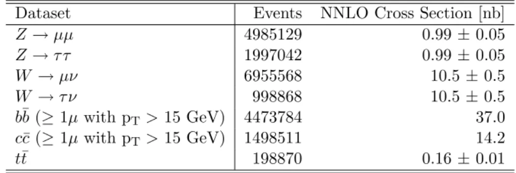
7.2 Data samples . . . . 56

7.2.1 Collision data . . . . 56

7.2.2 Monte Carlo data . . . . 57

7.3 Event selection . . . . 58

7.3.1 Good detector operating conditions . . . . 58

7.3.2 Trigger requirements . . . . 58

7.3.3 Primary vertex requirement . . . . 59

7.3.4 Event cleaning . . . . 59

7.4 Selection of physics objects . . . . 60

7.4.1 Muon selection . . . . 60

7.4.2 Electron selection . . . . 60

7.4.3 Hadronic τ decay selection . . . . 60

7.4.4 Lepton isolation . . . . 61

7.4.5 Requirement on Missing Transverse Energy . . . . 61

7.5 Z → τ τ event selection . . . . 65

7.5.1 Di-lepton veto . . . . 65

7.5.2 W background suppression cuts . . . . 65

7.5.3 Hadronic τ jet cleaning . . . . 69

7.5.4 Visible mass of the Z → τ τ final state . . . . 72

Contents ix

7.5.5 Results of the selection . . . . 72

7.6 Background estimation . . . . 80

7.6.1 Normalization of the W + jet background prediction to the data . . . . . 80

7.6.2 Normalization of the Z + jet background prediction to the data . . . . . 82

7.6.3 Estimation of the multi-jet background from data . . . . 82

7.7 Calculation of the Z → τ τ cross section . . . . 87

7.7.1 Results . . . . 88

7.7.2 Combination of the results and comparison with theoretical predictions . 89 7.8 Estimation of systematic uncertainties . . . . 92

7.8.1 Lepton reconstruction, isolation and trigger efficiency . . . . 92

7.8.2 τ trigger efficiency . . . . 92

7.8.3 Hadronic τ identification and misidentification rate . . . . 93

7.8.4 Lepton momentum resolution . . . . 93

7.8.5 Energy scale uncertainty . . . . 93

7.8.6 Cross section and luminosity . . . . 94

7.8.7 Systematic uncertainties on the background estimation . . . . 94

7.8.8 Systematic uncertainty on the acceptance . . . . 94

Conclusion and outlook 95

List of Figures 97

List of Tables 101

Acknowledgements 103

Bibliography 105

x Contents

You want to know how I did it?

This is how I did it, Anton:

I never saved anything for the swim back

Chapter 1

Introduction

The Standard Model describes with high accuracy the experimental observations in elementary particle physics. However there are aspects of the theory that are not confirmed experimentally yet. An important issue is the origin of the masses of elementary particles. In order to preserve the gauge invariance of the theory, fundamental particles are required to be massless. The Higgs mechanism gives masses to the particles without destroying the local gauge invariance by introducing a new scalar field, the Higgs boson field. The existence of the Higgs boson is not yet confirmed by experiments: its discovery or exclusion is one of the main goals of the experiments at the Large Hadron Collider (LHC) at CERN.

A brief introduction to the Standard Model is given in Chapter 2 together with a description of the phenomenology of the hadron collider physics.

The LHC is a proton proton collider with a maximal centre-of-mass energy of 14 TeV and a designed luminosity of 10 ³⁴ cm ⁻² s ⁻¹ . It is designed to discover and study new phenomena like supersymmetric particles and to give answers to open questions in our current understanding of the elementary particles and their interactions like the origin of particle masses and the existence of the Higgs boson.

One of the two general-purpose detectors of the LHC is the ATLAS detector. A brief description of the Large Hadron Collider and of the ATLAS detector is given in Chapter 3.

In Chapter 4, the muon spectrometer of the ATLAS experiment is described in detail. The muon spectrometer measures the momenta of muons emerging from the high energy interactions with a resolution of better than 10% up to 1 TeV. Final states with muons play an important role for the measurements in this thesis.

The main subject of this thesis is the measurement of the cross section of Z → τ τ production in proton-proton collisions at a centre-of-mass energy of 7 TeV with the ATLAS experiment.

The measurement of the inclusive Z cross section in τ τ final states can confirm the measurement in the electron and muon pair final states. The search for a low mass Higgs boson decaying into τ pairs requires knowledge of the Z → τ τ cross section. In addition, the selection of a clean sample of Z → τ τ events is instrumental for studies of the performance of the reconstruction of hadronic τ decays. In Chapter 5, the reconstruction of the electrons, muons and hadronic τ decays needed for the Z → τ τ event selection is described.

1

2 Chapter 1. Introduction

The measurement of inclusive Z → τ τ production can be performed in several final states depending on the decay modes of the τ leptons. The semileptonic final state with one τ lepton decaying into an electron or muon and neutrinos (τ _e , τ _µ ) and the other one into hadrons plus neutrino (τ _h ) is described in this thesis. The study of the muon reconstruction performance with the so-called tag-and-probe method using Z → µµ events is described in Chapter 6. It is mainly addressed to the Z → τ τ → τ _µ τ _h production, although many of the results can be extended to other processes involving muons.

The Z → τ τ decays are studied with data collected by the ATLAS experiment during 2011 corresponding to an integrated luminosity of 1.5 fb ⁻¹ . The selection of signal events, the estimation of the main backgrounds from data and the determination of the cross section including systematic uncertainties are described in Chapter 7.

The results presented in this thesis have been approved by the ATLAS Collaboration and

are published in [1].

Chapter 2

The Standard Model

The study of elementary particle physics began more than 100 years ago with the discovery of the electron. The analysis of the cosmic rays composition stimulated the curiosity of the scientific community at that time since the cosmic radiation was the only source of high energy particles. High energy accelerators were then developed, revealing a variety of new particles and exploring the structure of subnuclear matter.

The large variety of experimental data can be accounted for by the Standard Model of particle physics. The fundamental interactions relevant in particle physics are the electromagnetic, the weak and the strong force. At low energies these interactions appear to be completely unrelated.

For example, they have very different coupling strengths which give rise to interaction cross sections which differ by about 12 orders of magnitude. At very high energies, the coupling constants may, however, converge to a single value and interactions between elementary particles may be explained in terms of a single unified force.

In the 1960s a major breakthrough along the road to unification of the forces was made by Glashow [2], Weinberg [3] and Salam [4] when they unified the electromagnetic and weak interactions reinforcing the belief in the existence of a single unified theory of the fundamental interactions. The most significant theoretical step in this direction was the realization that all fundamental interactions are invariant under local gauge transformations.

In the Standard Model, all the interactions are described by three gauge symmetry groups, SU(3) _C ⊗ SU(2) _L ⊗ U(1) _Y

for the strong interaction (Quantum Chromodynamics) and the unified weak and electromagnetic interactions (Electroweak Theory). The electroweak SU (2) L ⊗ U (1) Y gauge symmetry is broken via the Higgs mechanism which predicts the existence of the Higgs field.

2.1 Particles and interactions

According to the Standard Model, matter is composed of fundamental particles with spin

⁄

(fermions): six quarks and six leptons with different masses and electric charges. Leptons exist

3

4 Chapter 2. The Standard Model

as free particles while quarks (a part from the top quark) are grouped into baryons consisting of 3 quarks or mesons, bound states of a quark and an anti-quark.

Interactions between particles are described by the exchange of a virtual spin 1 boson specific for the interaction. Three fundamental interactions are described by the Standard Model. The strong interaction is responsible for binding the quarks together within mesons and baryons and is mediated by eight massless particles, the gluons. The electromagnetic interaction is mediated by one massless boson, the photon. The weak interaction is, for example, responsible for the β decays of nuclei with the associated emission of neutrinos and is mediated by the massive W ^± and Z ⁰ bosons. The gravitational interaction is the weakest of all interactions. It cannot yet be described by a quantum field theory and, therefore, is not part of the Standard Model.

The elementary particles and interactions of the Standard Model are listed in Table 2.1.

Table 2.1: The fundamental particles and interactions described by the Standard Model.

Spin

⁄

Particle Q/|e|

Leptons e µ τ -1

ν e ν µ ν τ 0

Quarks u c t +2/3

d s b -1/3

Spin 1 Interaction Q/|e|

Gluon, g Strong 0

Photon, γ Electromagnetic 0 W ^± ,Z ⁰ Weak ±1, 0

Spin 0 Q/|e|

Higgs 0

2.2 Symmetries and conservation laws

The invariance of the equations that describe the physical system under symmetry transforma- tions is related to the conservation of physical quantities according to the Noether Theorem [5].

An example of such symmetry transformations are translations in space and time which corre- spond to the 4-momentum conservation.

The fundamental principle which determines the interactions of the Standard Model is the gauge symmetry, the invariance under continuous phase transformations of the matter field.

2.3 Quantum Chromodynamics

Quantum Chromodynamics (QCD) describes the strong interactions between colored quarks and gluons based on the SU(3) _C gauge symmetry. The color charge of the quarks can have three values called red, blue and green. The interaction is mediated by eight gluons carrying color and an anti-color quantum number and belonging to a SU(3) _C octet. A characteristic of the gluons in the SU(3) C gauge theory is their self-interaction due to their color charges.

At small distances, the interaction potential between quarks is Coulomb like, while it in- creases linearly at large distances leading to quark confinement :

V (r) = − 4 3

α S

r + kr

2.4. The Electroweak interaction 5

where α _S is the strong coupling and k is a phenomenological parameter. Free colored states do not exist. Increasing the distance between two color-charged particles leads to a linear increase in binding energy and eventually to the creation of quark-antiquark pairs from the vacuum.

These new quarks are grouped together with the initial partons in color-neutral bound states, the hadrons, which are observed. This process is called hadronization.

Quarks interact weakly at small distances and at high energies allowing for perturbative calculation of cross sections. This feature is called asymptotic freedom and is typical of non- Abelian gauge field theories, where the gauge bosons carry charges of the gauge groups and thus have self-coupling.

2.4 The Electroweak interaction

All leptons and quarks interact via the weak force. The original Fermi theory of the weak interaction describing nuclear β decay assumed point-like coupling between four fermions. A serious difficulty arises when the Fermi theory is applied to scattering processes at high energies.

The cross-section for elastic ν e -e scattering, for instance, is proportional to G ² s, where G is the weak Fermi coupling constant and s is the square of the centre-of-mass energy. The unitary violation at high energies can be avoided by introducing an intermediate gauge boson, the W ^± , as mediator of the weak interaction. The amplitude for this process to lowest order in perturbation theory is of the form

M = g

√

2 (J ^µ ) ^† 1 M _W ² − q ²

√ g

2 (J µ ) (2.1)

with the weak gauge coupling constant g and the mass of the W ^± boson M W . It is a product of a weak isospin current (J ^µ ) ^† , a charge-raising weak current J _µ , both of which behave like vectors and axial-vectors under Lorentz and parity transformations (V-A structure), and the W boson propagator. Processes with charge-changing currents are called charged current weak interactions and are mediated by the exchange of charged bosons, W ^± . The introduction of the charged weak bosons solved the unitarity violation of weak charged current processes. Weak neutral current processes like ν ν ¯ → W ⁺ W ⁻ required the introduction of an additional neutral gauge boson, Z ⁰ , to remove the unitary problem.

The Feynman graphs for electromagnetic and weak interactions between quarks and leptons show a strong similarity between them.

In 1960, Glashow [2], Weinberg [3] and Salam [4] described the electromagnetic and weak interactions within the framework of an unified electroweak gauge theory. In this theory, the weak coupling g is related to the electric charge by the relation

e = g sin θ _W (2.2)

where θ _W is the Weinberg mixing angle which has to be determined experimentally.

The electroweak theory requires four massless gauge bosons arranged in a weak isospin (I)

triplet W µ ⁽¹⁾ , W µ ⁽²⁾ , W µ ⁽³⁾ of the SU (2) L group, and a weak hypercharge (Y) singlet B µ of the

6 Chapter 2. The Standard Model

U (1) _Y group.

The weak SU (2) _L charge current interaction involves only left-handed fermions, while the electroweak neutral current U (1) Y interaction allows for both chirality.

The weak hypercharge Y is connected to the third component of the weak isospin I ₃ and the electric charge Q by the Gell-Mann-Nishijima relation for the electroweak theory:

Y = 2Q − 2I 3 . (2.3)

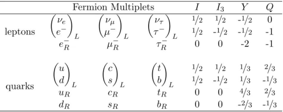
Leptons and quarks are arranged in multiplets of the electroweak gauge group. The quantum numbers of left- and right-handed fermions are summarized in Table 2.2.

The weak gauge boson field W _µ ^± and Z _µ ⁰ are massive while the photon field A µ remains massless. The physical boson fields (W _µ ^± , Z _µ ⁰ , A _µ ) are related to the components of the weak isospin triplet (W µ ⁽¹⁾ , W µ ⁽²⁾ , W µ ⁽³⁾ ) and weak hypercharge singlet (B µ ) by the following relations:

W _µ ⁺ = W µ ⁽¹⁾ √ + iW µ ⁽²⁾

2 , W _µ ⁻ = W µ ⁽¹⁾ √ − iW µ ⁽²⁾

2 , (2.4)

Z _µ ⁰ = cos θ _W W _µ ⁽³⁾ − sin θ _W B _µ , A _µ = sin θ _W W _µ ⁽³⁾ + cos θ _W B _µ . (2.5) Spontaneous breaking of the SU (2) L ⊗U (1) Y symmetry is required to provide masses to the gauge bosons, preserving the local gauge invariance of the Lagrangian and the renormalisability of the theory. This is achieved by the introduction of a new scalar field and the Higgs mechanism [6, 7, 8]

(see section 2.5).

Table 2.2: Fermion multiplets of the electroweak gauge group with their quantum numbers.

Fermion Multiplets I I 3 Y Q

leptons

ν e

e ⁻

L

ν µ

µ ⁻

L

ν τ

τ ⁻

L

1 / 2 1 / 2 - ¹ / 2 0

1 / 2 - ¹ / 2 - ¹ / 2 -1

e ⁻ _R µ ⁻ _R τ _R ⁻ 0 0 -2 -1

quarks

u d

L

c s

L

t b

L

1 / 2 1 / 2 1 / 3 2 / 3 1 / 2 - ¹ / 2 1 / 3 - ¹ / 3

u _R c _R t _R 0 0 ⁴ / 3 2 / 3

d R s R b R 0 0 - ² / 3 - ¹ / 3

2.5 The Higgs mechanism

The invariance of the electroweak Lagrangian under local gauge transformations demands mass-

less gauge bosons (W ^± and Z ⁰ ) and fermions, while the observed particles are massive. The

SU (2) _L ⊗ U(1) _Y gauge symmetry is spontaneously broken providing masses to the weak gauge

bosons and the fermions (Higgs mechanism).

2.5. The Higgs mechanism 7

The electroweak gauge symmetry is spontaneously broken by requiring the ground state of the system - the vacuum - to acquire a non-zero expectation value making it non-invariant under the gauge transformations.

At high energies (much greater than 100 GeV), the masses become negligible and the gauge symmetry is restored. At low energy, the symmetry is broken such that the weak W and Z bosons become massive, while the photon remains massless.

The Higgs mechanism introduces four scalar fields ϕ i arranged in a complex weak isospin doublet with hypercharge Y = 1:

ϕ = ϕ ⁺ ϕ ⁰

!

= 1

√ 2

ϕ 1 + iϕ ⁰ ₁ ϕ ₂ + iϕ ⁰ ₂

!

. (2.6)

The scalar Lagrangian invariant under SU (2) L ⊗ U (1) Y is

L = ( D µ ϕ) ^† ( D ^µ ϕ) − µ ² ϕ ^† ϕ − λ(ϕ ^† ϕ) ² (2.7) with the covariant derivative

D µ = ∂ _µ − gI · W _µ − (g ⁰ /2)Y B _µ . (2.8) with the weak charged and neutral current coupling constants g = _cos ^e _θ

W

and g ⁰ = _sinθ ^e

W

respectively. The first term in 2.7 is the kinetic term, while the second and third terms represent the self-interaction potential of the scalar field.

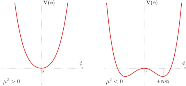
Figure 2.1 shows the potential for µ ² > 0 (left) and µ ² < 0 (right). The extremum at ϕ = 0 is not a minimum in the case of µ ² < 0 but there are minima for |ϕ| = ±υ = ± p

−µ ² /λ, where υ is the vacuum expectation value of the scalar field.

0

2

> 0

>

V()

+v 2 0

2

< 0

>

V()

/√

Figure 2.1: The Higgs potential for µ ² > 0 (left) and µ ² < 0 (right) [9]. In the latter case, the selection

of a particular ground state breaks the electroweak gauge symmetry of the Lagrangian.

8 Chapter 2. The Standard Model

The SU (2) _L ⊗ U (1) _Y symmetry is spontaneously broken when one of the ground states for µ ² < 0 is chosen. One can choose the vacuum state by selecting a specific direction in the space of the four scalar fields:

ϕ = 1

√ 2

0 υ

!

. (2.9)

Perturbation theory can be formulated in terms of excitations from the new ground state defined as the scalar Higgs boson field H(x). After a SU (2) _L gauge transformation eliminating the complex phase of the scalar field ϕ it can be parametrized as

ϕ(x) = 1

√ 2

0 υ + H(x)

!

. (2.10)

Equations 2.4, 2.5 and 2.10 are introduced into the Lagrangian 2.7, and the following expression for the kinetic term is obtained:

( D µ ϕ) ^† ( D ^µ ϕ) = g ² υ ²

8 (W _µ ⁺ W ^+µ + W _µ ⁻ W ^−µ ) + g ² υ ² 8 cos ² θ W

Z _µ Z ^µ . (2.11) which are mass terms for the W _µ ^± and Z µ fields. The gauge bosons W ^± and Z ⁰ acquire masses through the interaction with the Higgs field. The masses are given by the following relation:

m _Z cos θ _W = m _W = gυ

2 . (2.12)

The masses of the fermions are generated by the couplings of the fermions f to the Higgs field, which requires an additional term in the Lagrangian

L = −m _f f f ¯ − (g _f / √

2) ¯ f f H. (2.13)

for each fermion. The Lagrangian contains the fermion masses m _f = g _f υ/ √

2 and the fermion couplings g _f to the Higgs boson which are proportional to the fermion mass. Neutrinos do not couple to the Higgs boson in the original formulation of the theory without right-handed neutrino states.

2.6 Phenomenology of Z ⁰ boson productions at hadron colliders

The Glashow-Salam-Weinberg theory predicts the existence of the W ^± and Z ⁰ bosons and their properties. In 1983, the three weak gauge bosons have been discovered by the UA1 and UA2 experiments at CERN [10, 11, 12, 13] with the predicted properties.

The Z ⁰ boson can decay into fermion-antifermion pairs. In comparison to the W ^± produc-

tion, the Z ⁰ production cross section is about one-tenth. The Z ⁰ boson decays into lepton pairs

provide a clean signature for identification and can be reconstructed accurately. For this reason,

the measurement of the Z ⁰ decays is very important both for the test of the Standard Model

and for detector calibration.

2.6. Phenomenology of Z ⁰ boson productions at hadron colliders 9

A precise measurement of the Z ⁰ mass was performed by the four experiments (ALEPH, DELPHI, L3 and OPAL) [14] at the LEP, an electron-positron collider [15]:

M _Z

= 91.188 ± 0.002 GeV.

The branching ratios corresponding to the partial decay widths of the Z ⁰ are listed in Table 2.3.

Table 2.3: Partial widths and branching ratios decays [14].

Modes partial width (MeV) BR(Z ⁰ → X)%

e ⁺ e ⁻ 83.91 ± 0.12 3.363 ± 0.004 µ ⁺ µ ⁻ 83.99 ± 0.18 3.366 ± 0.007 τ ⁺ τ ⁻ 84.08 ± 0.22 3.367 ± 0.008 Hadrons 1744.4 ± 2.0 69.91 ± 0.06 Neutrinos 499.0 ± 1.5 20.00 ± 0.06

The cross section for Z production in proton proton collisions is calculated to NNLO in pertur- bation theory. The fundamental process is the q q ¯ → Z interaction:

σ _Z ^{q¯ q} = 8π 3

G F M _Z ²

√ 2 (g _V ² + g _A ² )δ(Q ² − M _Z ² ) (2.14) where Q ² = x _a x _b s, x _a and x _b the momentum fractions of the five quarks involved, s their centre- of-mass energy squared, g _V ² +g _A ² = (1 − 4|e _q | sin ² θ _W + 8e ² _q sin ⁴ θ _W )/8, e _q is the quark charge and θ W is the Weinberg angle. The Z ⁰ production cross section in proton-proton collisions is the convolution of the relation 2.14 with the quark and antiquark distribution functions q(x, Q ² ) in the proton, which give the probability to encounter a parton a with momentum fraction x _a :

σ ^pp→ZX = X

q

Z

dx _a dx _b [q(x _a , Q ² )¯ q(x _b , Q ² ) + a ↔ b]σ _Z ^{q¯ q} . (2.15) In addition to the primary “hard” interaction, many “soft” QCD interactions occur among the colliding and the spectator partons. The confinement of quarks and gluons requires that outgoing colored partons from the soft interactions undergo hadronization into colorless hadrons.

The Z ⁰ production cross section depends on the parton density functions (PDFs) of the

proton: different parametrization of the PDFs predict different Z boson production rates. The

differences between the predictions are taken into account as theoretical uncertainties.

10 Chapter 2. The Standard Model

Chapter 3

The ATLAS experiment at the Large Hadron Collider

In this chapter an overview of the ATLAS experiment at the Large Hadron Collider (LHC) [16]

at CERN is given.

On 20 November 2009, the LHC started to collide protons at a centre-of-mass energy of 900 GeV. On 30 March 2010, the LHC achieved with 7 TeV the highest center-of-mass energy ever reached at colliders. The LHC experiments collected data at 7 TeV in 2010 and 2011. From 2014, after further improvements of the accelerator, the LHC will run at its designed centre-of- mass energy of 14 TeV. The lower energy of 7 TeV is, however, sufficient to perform precision measurements of the Standard Model processes at the highest energies and to search for the Higgs boson and new physics beyond the Standard Model.

3.1 The Large Hadron Collider

The Large Hadron Collider (LHC) is the highest-energy particle accelerator. It is designed to accelerate proton beams up to an energy of 7 TeV per beam. For safety reasons, it started operation at a beam energy of only 3.5 TeV.

The LHC was built to test predictions of the Standard Model at the highest energies, to verify the existence of the Higgs boson and to search for new phenomena beyond the Standard Model.

The LHC is installed in a tunnel of 26.7 km circumference which housed the Large Electron Positron Collider (LEP) [15] until the year 2002.

In order to produce rare events with sufficient rate, the LHC is designed to reach a maximum luminosity of 10 ³⁴ cm ⁻² s ⁻¹ . The protons are kept on their circular path by superconducting dipole magnets which are cooled with liquid helium at 1.9 K temperature.

The event rate for a process with cross section σ is given by:

N = σ Z

Ldt = σL,

11

12 Chapter 3. The ATLAS experiment at the Large Hadron Collider

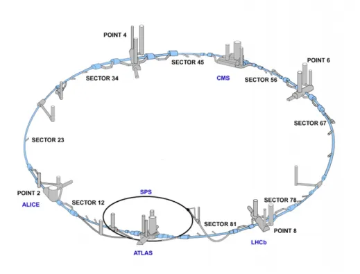
Figure 3.1: View of the LHC system.

where L is the instantaneous luminosity and L the integrated luminosity. The instantaneous luminosity is a parameter of the collider and depends on the beam shape and on the number of protons in each beam. At the design luminosity, the bunch crossing frequency is 40 MHz.

Figure 3.1 shows the LHC ring with the four detectors located at the interaction points:

The ATLAS Detector (A Toroidal LHC ApparatuS) [17] is one of the general purpose experiments. Data taken with the ATLAS detector are used for this thesis.

The CMS Detector (Compact Muon Solenoid) [18] is the second general purpose experiment.

Like ATLAS, it is designed to fully exploit the discovery potential of the LHC.

The ALICE Detector (A Large Ion Collider Experiment) [19] is designed to study the strong interaction and the Quark-Gluon Plasma (QGP) in heavy-ion (Pb-Pb) collisions.

The LHCb Detector (Large Hadron Collider beauty) [20] is a dedicated B-physics experi-

ment. The aim of the experiment is the search for new physics via precision measurements of CP

violating effects in B hadron decays and in rare decays, which are mostly produced in forward

direction with respect to the beam.

3.2. The ATLAS detector 13 Table 3.1: LHC beam parameters for the peak luminosity.

Unit Injection Collision Number of particles / bunch - 1.15 · 10 ¹¹

Number of bunches / beam - 2808

Circulating beam current (A) 0.582

Proton Energy (GeV) 450 7000

RMS transverse beam size (µm) 375.2 16.7

Stored beam energy (MJ) 23.3 362

Bunch crossing frequency (MHz) - 40

3.2 The ATLAS detector

ATLAS is composed of dedicated sub-detectors to fulfill the required tasks:

• The inner tracking system measures the tracks and momenta of charge particles and allows for the identification of electrons. In addition, decay vertices of particles are reconstructed accurately.

• The calorimeters identify electrons, photons and hadron jets and measure their energy and direction. With their good hermeticity and angular coverage they also allow for the measurement of missing transverse energy.

• The muon spectrometer identifies muons and measures precisely their momenta.

• A highly selective trigger system is required to suppress the huge background at the LHC.

3.2.1 The coordinate system

For the ATLAS detector the following right-handed coordinate system has been defined.

The z direction is parallel to the beam pipe with the origin located at the center of the detector. The x direction points to the center of the LHC ring, while the y axis points upwards.

The azimuthal angle φ and the polar angle θ are defined with respect to the z axis. Instead of the polar angle, the pseudorapidity η is frequently used at colliders:

η = −ln tan(θ/2).

Distances in the η-φ plane are given by

∆R = p

∆η ² + φ ² . 3.2.2 The magnet system

The ATLAS magnet system [21] consists of four superconducting magnets.

14 Chapter 3. The ATLAS experiment at the Large Hadron Collider

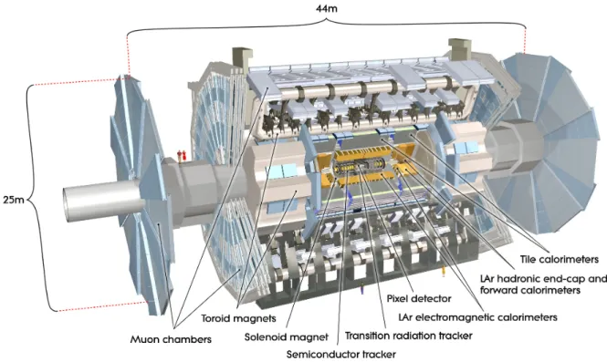
Figure 3.2: View of the ATLAS detector.

The central solenoid magnet surrounds the inner detector and provides a magnetic field strength of 2 T. The solenoid magnet operates at a temperature of 4 K. The solenoid coil extends 5.8 m in length and 2.6 m in diameter. Particles created at the interaction point are deflected by the solenoidal magnetic field in the R-φ plane.

Three air-core toroid magnets provide the magnetic field in the muon spectrometer. Each system (one in the barrel and two in the end-caps) is composed of eight coils. The air-core struc- ture is chosen to minimize the contribution of the multiple scattering to the muon momentum resolution. Details about the magnet system in the muon spectrometer are given in Chapter 4.

3.2.3 The Inner Detector

At the design luminosity of 10 ³⁴ cm ⁻² s ⁻¹ , the LHC proton beams will collide in ATLAS every 25 ns. At each bunch crossing, approximately 1000 tracks will emerge from the interaction point within |η| < 2.5. In the inner detector, fast and highly granular detectors are used to provide precise momentum measurement of charged particles as well as accurate reconstruction of secondary vertices close to the beam pipe.

The inner detector of ATLAS [22] is 7 m long and 2.30 m in diameter (Fig. 3.4). It is

composed of three sub-detectors, namely the silicon pixel detector, the semiconductor tracker

(SCT) and the transition radiation tracker (TRT). The goal of this detector is the reconstruction

and momentum measurement of charged particle tracks, for transverse momenta p T > 0.5 GeV

3.2. The ATLAS detector 15

Figure 3.3: View of the ATLAS magnet system.

within |η| < 2.5. In the solenoidal magnetic field of 2 T, a transverse momentum resolution of σ _p

/p _T = 0.05%p _T ⊕ 1%

is achieved. In addition, high precision in the reconstruction of secondary vertices is needed, in particular for the identification of b quark decays.

The pixel sub-detector is mounted close to the interaction point. It has very high granularity to achieve high spatial resolution close to the interaction point. The pixel detector is composed of three barrel layers at radii of 5, 9 and 12 cm, and five disks in each end-cap with radial extension from 11 to 20 cm completing the solid angle coverage. The innermost layer in the barrel, called b-layer, is crucial for the vertex location capabilities of the inner detector, especially for the reconstruction heavy flavor decays. Each pixel is 50 µm wide in R-φ and 400 µm long in z. The pixel detector provides an excellent position resolution of 10 µm in R-φ and 115 µm in z(R) in the barrel (endcap). Three space points are measured for a typical track crossing the pixel detector.

The pixel detector is surrounded by the semiconductor tracker (SCT) which is composed of four double layers of silicon strip detectors and typically provides four space points per track.

Each double layer contains strips aligned along the z direction and strips rotated by a stereo angle of 40 mrad with respect to the beam line providing z coordinate information. The strips have a pitch of 80 µm and are 12 cm long. The spatial resolution achieved by the SCT is 17 µm in R-φ and 580 µm in z (R) for the barrel (endcap) region.

The outermost tracking detector, the Transition Radiation Tracker (TRT), is composed of

36 layers of 4 mm diameter straw drift tubes. The small diameter allows for low occupancy and

high tracking efficiency and spacial resolution even at the high particle densities and rates at the

16 Chapter 3. The ATLAS experiment at the Large Hadron Collider

LHC. Electron identification is performed by using a Xe/CO ₂ /O ₂ gas mixture which is sensitive to the transition radiation photons created in radiator foils between the straws. Ultra-relativistic electrons passing through the numerous dielectric boundaries of these foils produce transition radiation which enhances ionization signal in the gas mixture. The large number of track points provides efficient track reconstruction within the TRT acceptance (|η| < 2.0). Each straw in the barrel part of the TRT provide an R-φ coordinate measurement with a precision of 130 µm.

Figure 3.4: Views of the ATLAS inner detector.

3.2.4 The Calorimeter System

The calorimeters are important for the reconstruction of many final states involving electrons, photons and hadron jets. In addition, they provide information about the missing transverse energy of the events and allow for the identification of hadronic τ decays.

The ATLAS detector contains an electromagnetic [23] and an hadron calorimeter [24]. Fi- gure 3.5 gives an overview of the ATLAS calorimeter system. All calorimeters are sampling calorimeters and provide full solid angle coverage up to |η| = 4.9.

The electromagnetic calorimeter uses liquid Argon as active medium and lead absorber plates

which, like the readout electrode boards, are accordion-shaped. The electromagnetic (EM)

calorimeter consists of a barrel part extending up to |η| = 1.5 and two end-caps (EMEC) up

to |η| = 3.2 which are complemented by two forward calorimeters in the region up to |η| =

4.9. The total thickness of the EM calorimeter is more than 24 radiation lengths (X ₀ ) in the

barrel and 26 radiation lengths in the end-caps. In the range |η| < 1.8, the calorimeter is

equipped with a presampling detector in front which provides an estimation of the energy losses

of electrons and photons before entering the calorimeter. The EM calorimeter is segmented

longitudinally along the particle direction in several layers in order to measure the longitudinal

shower profiles. Within |η| < 2.5 (the inner detector acceptance), there are three principal

shower samplings. The first layer is equipped with readout strips with a pitch of 4 mm in

η. This assures a precise position measurement in this direction and allows for good particle

3.2. The ATLAS detector 17

Table 3.2: Parameters for the ATLAS calorimeters. The energy resolutions are from test beam mea- surements [25, 27].

Name η range Absorber / active material Energy resolution

(stochastic) (constant)

EM <1.5 lead / LAr (10.1±0.4)%/ √

E (0.2±0.1)%

EMEC 1.5 - 3.2 lead / LAr (10.1±0.4)%/ √

E (0.2±0.1)%

Tile <1.7 steel / scint (52.0±1.0)%/ √

E (3.0±0.1)%

HEC 1.5 - 3.2 copper / LAr (70.6±1.5)%/ √

E (5.8±0.2)%

FCal1 3.2 - 4.9 copper / LAr (28.5±1.0)%/ √

E (3.5±0.1)%

FCal2+3 3.2 - 4.9 tung. / LAr (94.2±1.6)%/ √

E (7.5±0.14)%

identification. This layer acts as “preshower” detector with a thickness of 6 X 0 . The second layer is segmented into towers of size ∆η × ∆φ = 0.025 × 0.025. With a thickness of 16 X 0 , this is the largest which absorbs most of the electromagnetic energy of a shower. The third layer has coarser granularity and a thickness varying from 2 X 0 to 12 X 0 . This layer is used to estimate energy leakage of the EM showers into the subsequent hadron calorimeter. In the range 2.5

< |η| < 3.2, the electromagnetic end-cap (EMEC) calorimeters have a coarser granularity and only two samplings. In the forward range |η| > 3.2, a different type of liquid Argon calorimeters (FCAL) measures both the electromagnetic and the hadronic components of showers. They are longitudinally segmented into three different layers, each with a granularity of ∆η × ∆φ ≈ 0.2

× 0.2.

The hadron calorimeters (HCAL) surround the electromagnetic calorimeter. Their thickness of 11 interaction lengths is important to minimize the punch-through of hadrons into the muon spectrometer. Different technologies are used in different η-regions. For |η| < 1.6, an iron- scintillating-tile calorimeter is used in the barrel and extended barrel. The scintillation light is read out by photomultiplier tubes located behind each calorimeter module. In the region 1.5

< |η| < 3.2, liquid Argon is used as active material in combination with copper absorber plates used to increase the stopping power of the hadron calorimeter. The forward calorimeter uses Argon as active material embedded in a tungsten absorber matrix and extends the acceptance up to |η| = 4.9. The hadron end-cap and the forward calorimeter is placed in the same cryostat together with the EMEC calorimeter.

3.2.5 The Muon Spectrometer

The muon spectrometer [28] has been designed to fulfill the following requirements:

• Stand-alone identification and reconstruction of muons with high efficiency and a momen- tum resolution of better than 10% up to energies of 1 TeV. Multiple scattering is minimized by employing air-core toroid magnets.

• Coverage up to |η| = 2.7.

18 Chapter 3. The ATLAS experiment at the Large Hadron Collider

Figure 3.5: View of the ATLAS calorimeter system.

• Single and multiple muon trigger information with programmable momentum thresholds.

• Reliable operation and stable performance over a long period in a high irradiation envi- ronment.

Details about the muon spectrometer are given in Chapter 4.

3.3 Trigger and data acquisition

The majority of collisions at the LHC at a rate of 40 MHz is not interesting for the physics program and cannot be stored. On the other hand, interesting events must be kept.

The trigger selects interesting events out of the overwhelming background. The trigger selec-

tion proceeds in three consecutive levels, namely L1, L2 and the Event Filter. Each level refines

the trigger decision of the previous step. The first level (L1) is completely hardware based and

uses only limited amount of detector information in order to provide decisions within less than

2.5 µs. It uses information provided by the muon spectrometer and the calorimeters exploiting

not the full granularity. Events with high-p T muons, electrons, photons, jets and hadronically

decaying τ leptons as well as with large total and missing transverse energy are selected. The

associated Regions-of-Interest (RoI), i.e. the regions in the detector where interesting patterns

have been identified, are passed to the second trigger level (L2) at a rate of 75 kHz. The L2

selection criteria are chosen such that the event rate is reduced to 3.5 kHz at an event processing

time of 40 ms. For events selected by the L2 trigger, the full detector information is collected by

3.4. Luminosity monitoring 19

the Event Builder and passed to the Event Filter (EF). This last step is entirely software based.

Offline event reconstruction algorithms are employed and the final trigger decision is provided at an event processing time on the order of four seconds leading to a final event rate of 200 Hz recorded on mass-storage devices for further processing and physics analyses. The data volume recorded by the experiments at the LHC cannot be stored and processed at one local computing center alone. Therefore, after initial processing at CERN, the recorded data are distributed to many computing centers outside of CERN which together form the LHC Computing Grid (LCG), a worldwide computing framework [29].

3.4 Luminosity monitoring

The measurement of the cross sections of physics processes requires the knowledge of the lumi- nosity delivered by the LHC. An ATLAS run contains several Luminosity Blocks (LBs). A LB is a time interval (on the order of a minute) for which the integrated luminosity is determined.

By dividing a run into several LBs, ATLAS can process data more efficiently by removing any LBs affected by failures of detector components. Over each LB, the instantaneous luminosity is essentially constant.

The main detector for the ATLAS luminosity monitoring is LUCID (LUminosity measure- ment using ˇ Cerenkov Integrating Detector). LUCID also identifies individual bunch crossings.

LUCID detectors are placed at z = ± 17 m from the interaction point. The detectors consist of twenty 15 mm diameter drift tubes filled with C 4 F 10 . The drift tubes are arranged around the beam pipe at a radial distance of 10 cm.

The absolute luminosity is measured by ALFA (Absolute Luminosity For ATLAS) which is

located at a distance of 240 m from the interaction point. ALFA measures the elastic scattering

rate of proton-proton collisions which is related to the total cross section.

20 Chapter 3. The ATLAS experiment at the Large Hadron Collider

Chapter 4

The ATLAS Muon Spectrometer

Muon final states provide a clean and robust signature for many physics processes including those involving decays of new heavy particles. The muon spectrometer is a stand-alone detector which allows for the trigger and track measurement of the muons independently of the inner detector.

The acceptance of the muon spectrometer is |η| < 2.7.

Three superconducting air-core toroid magnets deflect the muons in the R-η plane.

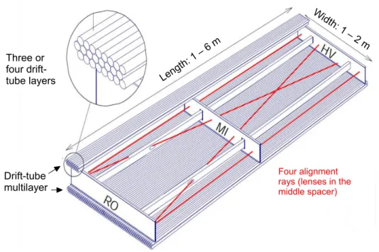
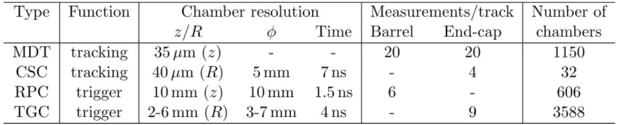
The muon spectrometer is equipped with three layers of Monitored Drift Tube (MDT) cham- bers in the barrel region, arranged in cylindrical layers around the beam axis. In the end-caps, MDT chambers are used together with Cathode Strip Chambers (CSC), arranged in wheels perpendicular to the beam axis.

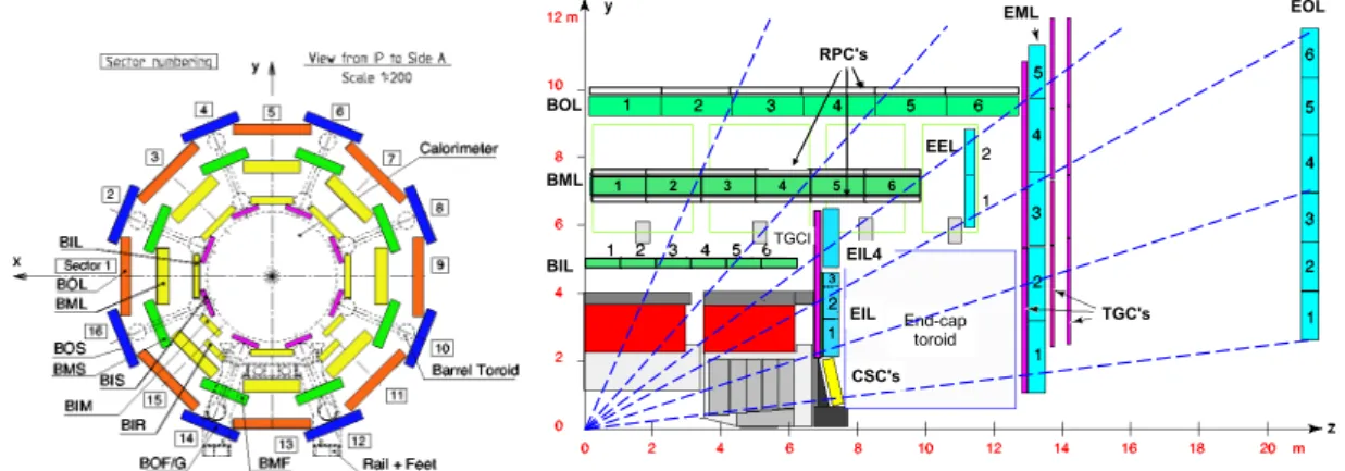
Resistive Plate Chambers (RPC) in the barrel middle and outer layers, and Thin Gap Cham- bers (TGC) in the end-cap inner and middle layers, complement the precision tracking chambers to provide measurement of the non-bending coordinate φ and to trigger on high-momentum muons. The acceptance of the muon trigger system is |η| < 2.4.

Figure 4.1: Cross sections of the muon spectrometer in the x-y plane (left) and in the y-z bending plane in the magnetic field (right).

21

22 Chapter 4. The ATLAS Muon Spectrometer

4.1 The toroid magnets

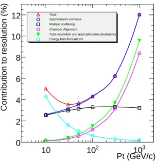
High momentum resolution is important for the precise reconstruction of muon final states. At low p T values, the muon momentum resolution is still dominated by multiple scattering (see Fig. 4.2) which is minimized by using air-core magnets for the muon spectrometer.

The magnet system is composed of three superconducting toroid magnets and covers the pseudorapidity range |η| < 2.7. The barrel toroid is 25 m long with an inner (outer) diameter of 9.4 (20.1) m. The end-cap toroids are placed at the ends of the barrel. They are 5 m long with an inner (outer) diameter of 1.65 (10.7) m. The toroidal magnetic fields provide a bending power of 3 Tm in the barrel and of 6 Tm in the end-caps.

4.2 The muon precision tracking chambers

The precision tracking chambers in the barrel are mounted in three cylindrical layers at radii of 5, 7.5 and 10 m. The overall coverage of the barrel detectors is |η| < 1. In the end-caps, the precision chambers are arranged in four disks at distances of 7, 10, 14 and 22 m from the interaction point. The coverage of the end-caps is 1 < |η| < 2.7. The precision chambers provide uniform coverage up to |η| = 2.7 within a gap at η = 0 where cables and services for the inner detector and the calorimeters are placed.

Figure 4.2 shows the different contributions to the muon momentum resolution. At high p T

values, the chamber resolution and alignment are the dominant contribution.

Pt (GeV/c)

10 10 ² 10 ³

Contribution to resolution (%)

0 2 4 6 8 10

12

Tube resolution and autocalibration (stochastic) Energy loss fluctuations

Figure 4.2: Contributions to the muon momentum resolution as a function of the transverse momentum.

4.2. The muon precision tracking chambers 23

4.2.1 Monitored Drift Tube (MDT) Chambers

The MDT chambers are the main muon tracking chambers both in the barrel and end-caps regions. A total of 1150 chambers covers an active area of 5500 m ² .

The basic elements of the MDT chambers are drift tubes with a diameter of 29.97 mm. The tube consists of aluminum with a wall thickness of 400 µm. The drift tubes are filled with Ar/CO ₂ (93/7) gas mixture at a pressure of 3 bar. At the center of each tube, a gold-plated tungsten-rhenium anode wire of 50 µm of diameter is located at a potential of 3080 V with respect to the tube wall creating a radial electric field.

When a muon traverses the drift gas, ion-electron pairs are created along its path. Secondary ionization is caused by the electrons produced in the primary ionization. Since secondary inte- ractions happen very close to the primary ionization, ion-electron pairs are grouped in clusters along the muon path. In the applied electric field, the electrons and ions drift towards the anode (wire) and cathode (tube wall), respectively, with average drift velocities. Near the wire, the electric field is high enough to accelerate the drifting electrons such that they ionize the Argon atoms of the gas creating an avalanche process. The electron amplification factor, the gas gain, depends on the gas mixture and pressure, and on the electric field strength near the wire. Since the avalanche is produced very close to the wire, the electron signal induced on the anode is very short and cannot be detected by the read-out electronics. Only the current signal induced by the secondary ions drifting from the avalanche region to the tube wall can be measured.

The determination of the position of a track in a drift tube is based on the measurement of the drift time of the primary ionization charge to the sense wire. It is defined as the time difference between the rising edge of the induced signal and the proton bunch crossing time of the LHC with corrections applied for the muon flight time from the interaction point to the muon detector and the signal propagation time along the wire. The drift time is converted into the drift radius, the distance of minimum approach between the muon trajectory and the anode wire, through the relation drift-time-space (r-t relation).

Gas mixture, pressure and the voltage applied to the drift tubes lead to a maximum drift time of about 700 ns. The corresponding gas gain is 2×10 ⁴ which is chosen to prevent aging of the drift tubes.

The drift tubes are arranged in several layers grouped into two multilayers mounted on an aluminum support frame. Each multilayer contains three tube layers in the middle and outer stations and four layers in the inner stations. Figure 4.3 shows the structure of an MDT chamber.

Each drift tube is read out at one end by a low-impedance preamplifier with programmable threshold, a shaper and a discriminator. An ADC measured the integrated signal charge. The drift tubes provide an average spatial resolution of 80 µm. The corresponding chamber resolution is 35 µm.

4.2.2 Cathode Strip Chambers (CSC)

The CSCs are gas ionization chambers consisting of four layers measuring the position of charged

particles via currents induced on pickup strips. They are installed in the region 2.0 < |η| < 2.7

24 Chapter 4. The ATLAS Muon Spectrometer

Figure 4.3: Schematics of an MDT chamber.

where the counting rate reaches 1700 Hz/cm ² . The ionization electron clusters are accelerated towards the anode wires, where the avalanche process occurs. The charge avalanche induces currents on two sets of cathode strips (192 strips orthogonal and 48 strips parallel to the wires) for each chamber. Each strip carries a fraction of the total induced current. The centroid of the charge of the affected adjacent strips measures the track coordinate. The drift time is 30 ns.

Spatial resolutions of 40 µm and 5 mm are achieved in R and φ, respectively.

4.3 Muon trigger chambers

The trigger chambers have to fulfill the following requirements:

• Bunch crossing identification requires a time resolution of better than the LHC bunch spacing time of 25 ns.

• High momentum muons are selected using a programable p _T threshold.

• Measurement of the bending and the non-bending coordinates with a resolution of 1 cm.

The ATLAS muon spectrometer employs Resistive Plate Chambers (RPC) in the barrel and Thin Gap Chambers (TGC) in the end-caps. Figure 4.4 shows the ATLAS muon trigger scheme.

In the barrel region (|η| < 1.05), three layers of RPCs are used, two (RPC1 and RPC2) beneath

and above the MDT chambers in the middle stations and the third (RPC3) together with the

outer MDT chambers. The trigger requires coincidences within predefined regions pointing to

4.3. Muon trigger chambers 25

Figure 4.4: The ATLAS muon trigger scheme.

the interaction region in both projections: coincidences in RPC1 and RPC2 for the low p _T trigger and with RPC3 in addition for the high p T trigger. In the end-cap region (1.05 < |η| <

2.4), three TGC trigger layers are installed in the middle chamber layer. The TGC layer in the inner end-cap layer is not used for the muon trigger but only for the measurement of the second coordinate.

Table 4.1 shows the performance of the four different sub-systems in the muon spectrometer.

Precision and trigger chambers provide the measurement of the position of muon tracks with good resolution in three dimensions.

Table 4.1: Performance of the chambers in the muon spectrometer.

Type Function Chamber resolution Measurements/track Number of

z/R φ Time Barrel End-cap chambers

MDT tracking 35 µm (z) - - 20 20 1150

CSC tracking 40 µm (R) 5 mm 7 ns - 4 32

RPC trigger 10 mm (z) 10 mm 1.5 ns 6 - 606

TGC trigger 2-6 mm (R) 3-7 mm 4 ns - 9 3588

26 Chapter 4. The ATLAS Muon Spectrometer

4.3.1 Resistive Plate Chambers (RPC)

The RPCs consist of a gas gap between two resistive Bakelite plates at a relative potential of 9.8 kV covered by two orthogonal series of pick-up strips. The η strips run parallel to the MDT wires and measure the track bending coordinate. The φ strips are orthogonal to the wires and provide the second coordinate.

The two Bakelite plates of 2 mm thickness are kept parallel using polycarbonate spacers of 12 mm diameter and 2 mm thickness. The gas mixture is C ₂ H ₂ F ₄ /Iso-C ₄ H ₁₀ /SF ₆ (94.7/5/0.3).

A uniform electric field of 4.9 kV/mm creates a discharge for a passing muon track.

4.3.2 Thin Gap Chambers (TGC)

The TGCs are multi-wire proportional chambers operating in saturation mode at a voltage of 2.9 kV. The distance between the wires is larger than the cathode-to-anode distance like in the CSCs. The wire-to-wire distance is 1.4 mm. The gas used is a mixture of 55% CO ₂ and 45%

n-C ₅ H ₁₂ (n-pentane). The anode wires are arranged parallel to the MDT wires. Pickup strips

provide the trigger information and the measurement of the non-bending coordinate.

Chapter 5

Reconstruction of physics observables

In this chapter, the main observables used for the ATLAS data analyses are described. Main emphasis is given to observables relevant for the Z → τ τ event selection.

5.1 Monte Carlo event generators and detector simulation

Several Monte Carlo generators are available to generate the physics processes as input for the ATLAS detector simulation. The simulation of physics processes in proton-proton collisions starts with the simulation of the hard scattering process followed by parton showering and the hadronization. In addition to the primary hard interaction also the underlying event, i.e.

interactions between the proton-remnants, are simulated. The events generated by the Monte Carlo generators are passed through the detailed simulation of the ATLAS [30] detector based on the GEANT4 [31] package for the description of the detector response.

Three Monte Carlo generators are employed for the analysis:

PYTHIA [32] is a general-purpose leading order (LO) generator for interactions in proton- proton collisions. This generator includes leading order matrix elements and simulates initial and final state QCD radiation as well as the underlying event and hadronization.

MC@NLO [33] is a Fortran package which combines a Monte Carlo event generator inclu- ding next to leading order (NLO) corrections for QCD processes. MC@NLO makes use of the Fortran HERWIG event generator [34] for the simulation of parton shower and hadronization processes.

ALPGEN [35] is a leading-order generator for physics processes at hadron colliders involving multi-parton interactions.

27

28 Chapter 5. Reconstruction of physics observables

5.2 Pile-up simulation

The cross section for inelastic pp interactions at the LHC at the center-of-mass energy of 7 TeV is 70 mb [36]. At the design luminosity of 10 ³⁴ cm ⁻² s ⁻¹ , the average number of minimum-bias events per bunch crossing is 23. Most of the particles produced in such interactions do not come from interesting physics processes. Due to the large number of protons per bunch, at each bunch crossing multiple inelastic pp interactions overlay the interesting physics processes selected by the trigger system. This effect is referred to as in-time pile-up.

The average number of interactions per bunch crossing scales linearly with the luminosity.

In addition, the electronic signals are integrated over several bunch crossings leading to the so called out-of-time pileup. The out-of-time pile-up depends on the time between bunch crossings and on the electronic integration times which differs for the different detector subsystems.

The effect of the in-time pile-up increases the observed energy measured in the calorimeters.

The out-of-time pileup decreases the observed energy in the calorimeters, due to the negative tail in the LAr pulse shape and also increases the noise.

Usually, Monte Carlo samples are produced before or during a given data taking period. By that design, only a best-guess of the data pileup conditions can be put into the simulation. Since 2011 data taking, LHC is running with bunch trains with an in-train bunch separation of 50 ns, then also the out-of-time pile-up effect needs to be taken into account.

At the analysis level, simulated events need to be re-weighted according to the pile-up con- ditions found in data. The commonly used variables for the re-weighting procedure in Monte Carlo are:

• number of primary vertices to measure the activity in the current bunch-crossing: sensitive only to in-time pileup.

• average interaction per bunch-crossing (µ) calculated from luminosity for each luminosity block (LB): average of in-time and out-of-time pileup. The µ value is calculated with the average across all bunch crossing IDs (BCIDs) in the LB. An alternative procedure calculates the µ values for each BCID.

5.3 Particle reconstruction and identification

5.3.1 Electrons

Reconstruction and identification of electrons is needed in many physics analyses. A good

understanding of the combined performance of the inner detector and calorimeters allows a

good rejection against jets and background electrons from photon conversion. The definition

of electrons is performed in two steps: reconstruction of the electron track and calorimeter

deposition and identification. Three different algorithms have been developed for the electron

reconstruction. The main algorithm is dedicated to high p _T isolated electrons and requires

measurements both in the inner detector and LAr calorimeter. A second algorithm is mostly

dedicated to low p T electrons and electrons in jets. This algorithm is seeded by inner detector

5.3. Particle reconstruction and identification 29

tracks. The third algorithm is used for the reconstruction of forward electrons where no track matching is required due to the limited coverage of the inner detector.

In the following, only the first algorithm is described, since this is used for the electron selection in the Z → τ τ analysis presented in this thesis.

Reconstruction The main reconstruction algorithm for isolated electrons is based on clusters in the electromagnetic calorimeter associated to tracks reconstructed in the inner detector. Seed clusters with energies greater than 2.5 GeV are formed by a sliding window algorithm. A window of size N η × N φ (3×5) cells is slid across the η-φ grid of the LAr calorimeter to find energy depositions above a predefined threshold. Those seeds are used to build clusters by scanning the calorimeter layers for associated energy deposits and determining their energy and position. Reconstructed tracks are matched to the seed clusters by extrapolating the last point measured in the inner detector to the second layer of the LAr calorimeter. The match is performed comparing η and φ coordinates of the track and cluster candidates. If the track candidate has no hits in the silicon tracker, the match with the cluster is performed only in the φ coordinate, since the η coordinate measured by the TRT is not accurate enough. Matching tracks and clusters are considered as electron candidates. The electromagnetic cluster is then redetermined using a 3×7 (5×5) sliding window in the barrel (end-cap). The energy of the electron candidate is calculated as the weighted average of the cluster energy and the observed track momentum. The φ and η are taken from the track parameters. If there is no silicon detector hits, the η coordinate is taken from the reconstructed cluster position.

Identification The identification procedure aims at a good separation of isolated electrons and jets (faking electrons). The variables used for the identification are taken from track and cluster parameters. According to the signal efficiency and background rejection required for specific physics analyses, loose, medium or tight selection criteria are used. The loose identification is performed using the shower profile of the cluster in the second layer of the calorimeters and the energy deposition leakage into the hadronic calorimeter. The medium identification uses in addition information from the first layer of the calorimeter and track quality and tighter track- cluster matching requirements. The tight selection further applies cuts on the ratio between the energy deposition in the calorimeter and the momentum of the electron track and requires b-layer hits and the electron identification in the TRT using multivariate analysis methods.

Details on the electron identification together with performance of the identification algo- rithms can be found in [37].

5.3.2 Muons

The ATLAS muon spectrometer is designed to reconstruct and identify muons with better than 95% efficiency over a wide transverse momentum and solid angle range (|η| < 2.7) and with a muon momentum resolution of better than 10% for transverse momenta up to 1 TeV.

The so-called stand-alone muon reconstruction uses only track segments in the muon spec-

trometer up to |η| < 2.7. The muon trajectory in the bending plane (R-η) is calculated from