TheOPALCollaboration τ Leptons AMeasurementofthe τ MassandtheFirstCPTTestwith

arXiv:hep-ex/0005009v1 4 May 2000

EUROPEAN ORGANIZATION FOR NUCLEAR RESEARCH

CERN-EP-2000-056 April 26, 2000

A Measurement of the τ Mass

and the First CPT Test with τ Leptons

The OPAL Collaboration

Abstract

We measure the mass of the τ lepton to be 1775.1 ± 1.6(stat.) ± 1.0(sys.) MeV using τ pairs from Z ⁰ decays. To test CPT invariance we compare the masses of the positively and negatively charged τ leptons. The relative mass difference is found to be smaller than 3.0 × 10 ^{− 3} at the 90 % confidence level.

(Submitted to Physics Letters B)

The OPAL Collaboration

G. Abbiendi ² , K. Ackerstaff ⁸ , C. Ainsley ⁵ , P.F. Akesson ³ , G. Alexander ²² , J. Allison ¹⁶ ,

K.J. Anderson ⁹ , S. Arcelli ¹⁷ , S. Asai ²³ , S.F. Ashby ¹ , D. Axen ²⁷ , G. Azuelos ^18,a , I. Bailey ²⁶ , A.H. Ball ⁸ , E. Barberio ⁸ , R.J. Barlow ¹⁶ , J.R. Batley ⁵ , S. Baumann ³ , T. Behnke ²⁵ , K.W. Bell ²⁰ , G. Bella ²² , A. Bellerive ⁹ , S. Bentvelsen ⁸ , S. Bethke ^14,i , O. Biebel ^14,i , I.J. Bloodworth ¹ , P. Bock ¹¹ , J. B¨ohme ^14,h ,

O. Boeriu ¹⁰ , D. Bonacorsi ² , M. Boutemeur ³¹ , S. Braibant ⁸ , P. Bright-Thomas ¹ , L. Brigliadori ² , R.M. Brown ²⁰ , H.J. Burckhart ⁸ , J. Cammin ³ , P. Capiluppi ² , R.K. Carnegie ⁶ , A.A. Carter ¹³ , J.R. Carter ⁵ , C.Y. Chang ¹⁷ , D.G. Charlton ^1,b , C. Ciocca ² , P.E.L. Clarke ¹⁵ , E. Clay ¹⁵ , I. Cohen ²² ,

O.C. Cooke ⁸ , J. Couchman ¹⁵ , C. Couyoumtzelis ¹³ , R.L. Coxe ⁹ , M. Cuffiani ² , S. Dado ²¹ , G.M. Dallavalle ² , S. Dallison ¹⁶ , R. Davis ²⁸ , A. de Roeck ⁸ , P. Dervan ¹⁵ , K. Desch ²⁵ , B. Dienes ^30,h ,

M.S. Dixit ⁷ , M. Donkers ⁶ , J. Dubbert ³¹ , E. Duchovni ²⁴ , G. Duckeck ³¹ , I.P. Duerdoth ¹⁶ ,

P.G. Estabrooks ⁶ , E. Etzion ²² , F. Fabbri ² , M. Fanti ² , A.A. Faust ²⁸ , L. Feld ¹⁰ , P. Ferrari ¹² , F. Fiedler ⁸ , I. Fleck ¹⁰ , M. Ford ⁵ , A. Frey ⁸ , A. F¨ urtjes ⁸ , D.I. Futyan ¹⁶ , P. Gagnon ¹² , J.W. Gary ⁴ , G. Gaycken ²⁵ , C. Geich-Gimbel ³ , G. Giacomelli ² , P. Giacomelli ⁸ , D.M. Gingrich ^28,a , D. Glenzinski ⁹ , J. Goldberg ²¹ ,

C. Grandi ² , K. Graham ²⁶ , E. Gross ²⁴ , J. Grunhaus ²² , M. Gruw´e ²⁵ , P.O. G¨ unther ³ , C. Hajdu ²⁹ G.G. Hanson ¹² , M. Hansroul ⁸ , M. Hapke ¹³ , K. Harder ²⁵ , A. Harel ²¹ , C.K. Hargrove ⁷ , M. Harin-Dirac ⁴ , A. Hauke ³ , M. Hauschild ⁸ , C.M. Hawkes ¹ , R. Hawkings ²⁵ , R.J. Hemingway ⁶ , C. Hensel ²⁵ , G. Herten ¹⁰ ,

R.D. Heuer ²⁵ , M.D. Hildreth ⁸ , J.C. Hill ⁵ , P.R. Hobson ²⁵ , A. Hocker ⁹ , K. Hoffman ⁸ , R.J. Homer ¹ , A.K. Honma ⁸ , D. Horv´ ath ^29,c , K.R. Hossain ²⁸ , R. Howard ²⁷ , P. H¨ untemeyer ²⁵ , P. Igo-Kemenes ¹¹ , D.C. Imrie ²⁵ , K. Ishii ²³ , F.R. Jacob ²⁰ , A. Jawahery ¹⁷ , H. Jeremie ¹⁸ , C.R. Jones ⁵ , P. Jovanovic ¹ ,

T.R. Junk ⁶ , N. Kanaya ²³ , J. Kanzaki ²³ , G. Karapetian ¹⁸ , D. Karlen ⁶ , V. Kartvelishvili ¹⁶ , K. Kawagoe ²³ , T. Kawamoto ²³ , P.I. Kayal ²⁸ , R.K. Keeler ²⁶ , R.G. Kellogg ¹⁷ , B.W. Kennedy ²⁰ , D.H. Kim ¹⁹ , K. Klein ¹¹ , A. Klier ²⁴ , T. Kobayashi ²³ , M. Kobel ³ , T.P. Kokott ³ , S. Komamiya ²³ , R.V. Kowalewski ²⁶ , T. Kress ⁴ , P. Krieger ⁶ , J. von Krogh ¹¹ , T. Kuhl ³ , M. Kupper ²⁴ , P. Kyberd ¹³ , G.D. Lafferty ¹⁶ , H. Landsman ²¹ , D. Lanske ¹⁴ , I. Lawson ²⁶ , J.G. Layter ⁴ , A. Leins ³¹ , D. Lellouch ²⁴ ,

J. Letts ¹² , L. Levinson ²⁴ , R. Liebisch ¹¹ , J. Lillich ¹⁰ , B. List ⁸ , C. Littlewood ⁵ , A.W. Lloyd ¹ , S.L. Lloyd ¹³ , F.K. Loebinger ¹⁶ , G.D. Long ²⁶ , M.J. Losty ⁷ , J. Lu ²⁷ , J. Ludwig ¹⁰ , A. Macchiolo ¹⁸ ,

A. Macpherson ²⁸ , W. Mader ³ , M. Mannelli ⁸ , S. Marcellini ² , T.E. Marchant ¹⁶ , A.J. Martin ¹³ , J.P. Martin ¹⁸ , G. Martinez ¹⁷ , T. Mashimo ²³ , P. M¨attig ²⁴ , W.J. McDonald ²⁸ , J. McKenna ²⁷ , T.J. McMahon ¹ , R.A. McPherson ²⁶ , F. Meijers ⁸ , P. Mendez-Lorenzo ³¹ , F.S. Merritt ⁹ , H. Mes ⁷ , A. Michelini ² , S. Mihara ²³ , G. Mikenberg ²⁴ , D.J. Miller ¹⁵ , W. Mohr ¹⁰ , A. Montanari ² , T. Mori ²³ , K. Nagai ⁸ , I. Nakamura ²³ , H.A. Neal ^12,f , R. Nisius ⁸ , S.W. O’Neale ¹ , F.G. Oakham ⁷ , F. Odorici ² ,

H.O. Ogren ¹² , A. Oh ⁸ , A. Okpara ¹¹ , M.J. Oreglia ⁹ , S. Orito ²³ , G. P´ asztor ⁸ , J.R. Pater ¹⁶ , G.N. Patrick ²⁰ , J. Patt ¹⁰ , P. Pfeifenschneider ¹⁴ , J.E. Pilcher ⁹ , J. Pinfold ²⁸ , D.E. Plane ⁸ , B. Poli ² ,

J. Polok ⁸ , O. Pooth ⁸ , M. Przybycie´ n ^8,d , A. Quadt ⁸ , C. Rembser ⁸ , H. Rick ⁴ , S.A. Robins ²¹ , N. Rodning ²⁸ , J.M. Roney ²⁶ , S. Rosati ³ , K. Roscoe ¹⁶ , A.M. Rossi ² , Y. Rozen ²¹ , K. Runge ¹⁰ , O. Runolfsson ⁸ , D.R. Rust ¹² , K. Sachs ⁶ , T. Saeki ²³ , O. Sahr ³¹ , W.M. Sang ²⁵ , E.K.G. Sarkisyan ²² ,

C. Sbarra ²⁶ , A.D. Schaile ³¹ , O. Schaile ³¹ , P. Scharff-Hansen ⁸ , S. Schmitt ¹¹ , M. Schr¨ oder ⁸ , M. Schumacher ²⁵ , C. Schwick ⁸ , W.G. Scott ²⁰ , R. Seuster ^14,h , T.G. Shears ⁸ , B.C. Shen ⁴ , C.H. Shepherd-Themistocleous ⁵ , P. Sherwood ¹⁵ , G.P. Siroli ² , A. Skuja ¹⁷ , A.M. Smith ⁸ , G.A. Snow ¹⁷ , R. Sobie ²⁶ , S. S¨ oldner-Rembold ^10,e , S. Spagnolo ²⁰ , M. Sproston ²⁰ , A. Stahl ³ , K. Stephens ¹⁶ , K. Stoll ¹⁰ ,

D. Strom ¹⁹ , R. Str¨ ohmer ³¹ , B. Surrow ⁸ , S.D. Talbot ¹ , S. Tarem ²¹ , R.J. Taylor ¹⁵ , R. Teuscher ⁹ , M. Thiergen ¹⁰ , J. Thomas ¹⁵ , M.A. Thomson ⁸ , E. Torrence ⁹ , S. Towers ⁶ , T. Trefzger ³¹ , I. Trigger ⁸ , Z. Tr´ ocs´ anyi ^30,g , E. Tsur ²² , M.F. Turner-Watson ¹ , I. Ueda ²³ , P. Vannerem ¹⁰ , M. Verzocchi ⁸ , H. Voss ⁸ ,

J. Vossebeld ⁸ , D. Waller ⁶ , C.P. Ward ⁵ , D.R. Ward ⁵ , P.M. Watkins ¹ , A.T. Watson ¹ , N.K. Watson ¹ , P.S. Wells ⁸ , T. Wengler ⁸ , N. Wermes ³ , D. Wetterling ¹¹ J.S. White ⁶ , G.W. Wilson ¹⁶ , J.A. Wilson ¹ ,

16 23 18 8

1 School of Physics and Astronomy, University of Birmingham, Birmingham B15 2TT, UK

2 Dipartimento di Fisica dell’ Universit` a di Bologna and INFN, I-40126 Bologna, Italy

3 Physikalisches Institut, Universit¨ at Bonn, D-53115 Bonn, Germany

4 Department of Physics, University of California, Riverside CA 92521, USA

5 Cavendish Laboratory, Cambridge CB3 0HE, UK

6 Ottawa-Carleton Institute for Physics, Department of Physics, Carleton University, Ottawa, Ontario K1S 5B6, Canada

7 Centre for Research in Particle Physics, Carleton University, Ottawa, Ontario K1S 5B6, Canada

8 CERN, European Organization for Nuclear Research, CH-1211 Geneva 23, Switzerland

9 Enrico Fermi Institute and Department of Physics, University of Chicago, Chicago IL 60637, USA

10 Fakult¨at f¨ ur Physik, Albert Ludwigs Universit¨ at, D-79104 Freiburg, Germany

11 Physikalisches Institut, Universit¨ at Heidelberg, D-69120 Heidelberg, Germany

12 Indiana University, Department of Physics, Swain Hall West 117, Bloomington IN 47405, USA

13 Queen Mary and Westfield College, University of London, London E1 4NS, UK

14 Technische Hochschule Aachen, III Physikalisches Institut, Sommerfeldstrasse 26-28, D-52056 Aachen, Germany

15 University College London, London WC1E 6BT, UK

16 Department of Physics, Schuster Laboratory, The University, Manchester M13 9PL, UK

17 Department of Physics, University of Maryland, College Park, MD 20742, USA

18 Laboratoire de Physique Nucl´eaire, Universit´e de Montr´eal, Montr´eal, Quebec H3C 3J7, Canada

19 University of Oregon, Department of Physics, Eugene OR 97403, USA

20 CLRC Rutherford Appleton Laboratory, Chilton, Didcot, Oxfordshire OX11 0QX, UK

21 Department of Physics, Technion-Israel Institute of Technology, Haifa 32000, Israel

22 Department of Physics and Astronomy, Tel Aviv University, Tel Aviv 69978, Israel

23 International Centre for Elementary Particle Physics and Department of Physics, University of Tokyo, Tokyo 113-0033, and Kobe University, Kobe 657-8501, Japan

24 Particle Physics Department, Weizmann Institute of Science, Rehovot 76100, Israel

25 Universit¨ at Hamburg/DESY, II Institut f¨ ur Experimental Physik, Notkestrasse 85, D-22607 Ham- burg, Germany

26 University of Victoria, Department of Physics, P O Box 3055, Victoria BC V8W 3P6, Canada

27 University of British Columbia, Department of Physics, Vancouver BC V6T 1Z1, Canada

28 University of Alberta, Department of Physics, Edmonton AB T6G 2J1, Canada

29 Research Institute for Particle and Nuclear Physics, H-1525 Budapest, P O Box 49, Hungary

30 Institute of Nuclear Research, H-4001 Debrecen, P O Box 51, Hungary

31 Ludwigs-Maximilians-Universit¨ at M¨ unchen, Sektion Physik, Am Coulombwall 1, D-85748 Garching, Germany

a and at TRIUMF, Vancouver, Canada V6T 2A3

b and Royal Society University Research Fellow

c and Institute of Nuclear Research, Debrecen, Hungary

d and University of Mining and Metallurgy, Cracow

e and Heisenberg Fellow

f now at Yale University, Dept of Physics, New Haven, USA

g and Department of Experimental Physics, Lajos Kossuth University, Debrecen, Hungary

h and MPI M¨ unchen

i now at MPI f¨ ur Physik, 80805 M¨ unchen.

1 Introduction

We have measured the mass of the τ lepton, m τ , using data taken by the OPAL detector during LEP running at the Z ⁰ resonance. The first test of CPT invariance using τ leptons is performed by measuring the masses of the positively and negatively charged τ leptons separately. To determine the τ mass we use two pseudomass techniques, previously established by ARGUS [1]

and CLEO [2], which rely on the reconstruction of the mass, energy, and direction of the hadronic system in hadronic τ decays.

In the OPAL detector charged particle tracks are reconstructed by a central detector consist- ing of a silicon microvertex detector, a vertex chamber, a large jet chamber, and z-chambers.

Photons coming from the decay of neutral pions are measured using a hermetic lead glass calorimeter located outside of the solenoid and an iron–streamer tube sandwich calorimeter is used to measure hadronic showers. This hadronic calorimeter is used in conjunction with muon chambers mounted around it to separate muons from hadrons in the event selection and decay mode identification. The OPAL detector is described in detail elsewhere [3].

2 The Pseudomass Method

In a hadronic τ decay, the mass of the τ lepton is related to the 4-momentum of the resulting hadronic system ¹ by the formula

m ² _ν = (p τ − p h ) ² = m ² _τ − 2E τ E h + 2 | ~p τ || ~p h | cos ψ + m ² _h , | ~p τ | = p

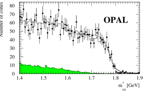
E _τ ² − m ² _τ (1) where p τ (p h ), p ~ τ (~p h ), and E τ (E h ) are the 4-momentum, 3-momentum, and energy of the τ (hadronic system). The neutrino mass, m ν , is set to zero and the τ energy is taken to be the beam energy, thus permitting the mass of the τ lepton to be reconstructed if the angle ψ between the direction of the τ and the hadronic system were known. Due to the high boost at LEP energies, ψ is limited to a few degrees, with the exact limit on ψ depending on m h . A pseudomass, m ^∗ _cn (one value per cone ² ), is defined by taking ψ to be zero. It gives the true mass when ψ = 0 and is smaller than the true mass in any other case. The distribution of m ^∗ _cn for τ → 3 π ^± ν τ decays, presented in fig. 1 is a broad distribution with a sharp cutoff at the τ mass. Further, the details of the shape of the distribution are determined by the dynamics of the decay with the general tendency that the more massive the hadronic system, the closer the pseudomass is to the cutoff. However, the position of the cutoff only depends on the mass of the τ lepton. The τ mass is extracted from this position. From fig. 1 a small tail of pseudomass above the cutoff is evident. It is caused by three effects: background, resolution, and initial state radiation, the latter weakens the assumption E τ = E beam . More details can be found in [1].

1

Here ‘hadronic system’ is defined as the sum of all the hadrons produced in the decay. The sum of their momenta gives the momentum of the hadronic system.

2

Cones with a half-opening angle of 35

are defined around the leading particles in the event. In most cases

a cone contains the decay products of exactly one τ.

m cn

* [GeV]

Number of cones

OPAL

0 10 20 30 40 50 60 70 80

1.4 1.5 1.6 1.7 1.8 1.9

Figure 1: The distribution of the pseudomass m ^∗ _cn from the τ → 3 π ^± ν τ class. The points with error bars are data and the open histogram is the Monte Carlo prediction including the background from misidentified τ decays (shaded area) normalized to the data. The solid line shows the parameterization in the fit window (1.6 to 2.0 GeV) after the final unbinned maximum likelihood fit to the data. The events have been binned for the presentation only.

In τ pair events where both τ leptons decay hadronically, a second pseudomass, m ^∗ _ev , can be defined, which is derived from the event as a whole, not just from one of the two cones.

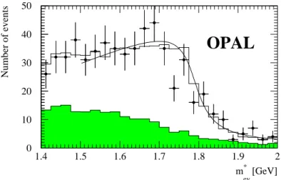
In such events the acollinearity α, i.e. the angle between the hadronic systems from the two decays, carries additional information on the τ mass (see fig. 2). This acollinearity restricts the decay angles of the τ leptons through the relation ψ ₊ + ψ ⁻ + α ≥ π, where ψ ₊ and ψ ⁻ are the decay angles of the positive and negative τ in the laboratory frame, respectively. If the sum of these three angles were known, the mass of the τ lepton could be reconstructed on an event by event basis. Since this information is unavailable the pseudomass, m ^∗ _ev , is calculated instead, assuming that the sum of the three angles is 180 degrees and that the masses of the positive and negative τ are equal. The m ^∗ _ev distribution shows similar features to m ^∗ _cn . An example is shown in fig. 3. Again, the cutoff at high values, from which the τ mass is extracted, is clearly visible. More details can be found in [2].

α τ

00000 00000 11111 11111

τ ^ψ

h

h ⁺

ψ

+

-

+

- ^-

Figure 2: Illustration of the relevant angles: ψ + and ψ ⁻ are the opening angles between the τ lepton and its hadronic decay products. α is the angle between the hadrons of the two τ leptons. In the absence of radiation, the τ leptons are produced collinear.

2

m

*

[GeV]

Number of events

OPAL

0 10 20 30 40 50

1.4 1.5 1.6 1.7 1.8 1.9 2

Figure 3: The distribution of the pseudomass m ^∗ _ev from the class of τ → π ^± ν τ decays recoiling against τ → π ^± π ⁰ ν τ . The points with error bars are data and the open histogram is the Monte Carlo prediction including the background from misidentified τ decays (shaded area) normalized to the data. The solid line shows the parameterization in the fit window (1.5 to 2.0 GeV) after the final unbinned maximum likelihood fit to the data. The events have been binned for the presentation only.

3 Selection and Classification

The selection of τ pair events is performed as described in [4] using the data recorded during the years 1990 to 1995 at center-of-mass energies at and around the Z ⁰ mass. A total of 159 373 τ pairs are identified within a geometrical acceptance limited to polar angles ³ of | cos θ | < 0.95.

The overall efficiency including the geometrical acceptance is 89 %. The purity of the sample is 98 %. The background consists mainly of electron and muon pairs.

Each selected event is split into two narrow cones of particles, one for each τ . All 1-prong and 3-prong cones ⁴ with a minimum momentum of 5 % of the beam momentum are then subjected to a likelihood classification in order to identify the decay mode of the two τ leptons using the same procedure as in [5]. Table 1 summarizes the decay modes considered.

For the calculation of the pseudomasses m ^∗ _cn and m ^∗ _ev , all tracks are assumed to origi- nate from charged pions. Neutral pions are reconstructed from showers in the electromagnetic calorimeter with the algorithm described in [5]. The number of neutral pions reconstructed in a cone does not necessarily match the number of π ⁰ expected from the decay mode identified by the likelihood selection. For example, there might only be a single π ⁰ reconstructed in a cone identified as a τ → π ^± 2 π ⁰ ν τ decay. In such a case the missing neutral pions are ignored in the calculation of the 4-momentum of the hadronic system. If there are too many π ⁰ reconstructed, we exclude those with the lowest energies.

3

We use a righthanded coordinate system with the z-axis pointing in the direction of the electron beam and the x-axis pointing towards the center of LEP.

4

A 1- or 3-prong cone is a cone containing 1 or 3 charged tracks.

1-prong modes 3-prong modes

eff. % pur. % decays eff. % pur. % decays

τ → π ^± ν τ 76.2 % 64.5 % 41148 τ → 3 π ^± ν τ 71.5 % 83.8 % 24832 τ → π ^± π ⁰ ν τ 60.2 % 77.1 % 58518 τ → 3 π ^± π ⁰ ν τ 61.6 % 64.2 % 11636 τ → π ^± 2 π ⁰ ν τ 45.1 % 40.9 % 26093

Table 1: Efficiency, purity, and number of decays selected by the likelihood identification in the decay modes explored in this analysis. In addition to these modes, the likelihood identifies leptonic decays and various modes with one charged hadron plus additional tracks from photon conversions or Dalitz decays. All numbers refer to the full range of pseudomasses. The purity in the region of the cutoff is substantially better.

π ^± π ^± π ⁰ π ^± 2π ⁰ 3 π ^± 3π ^± π ⁰

no ID – – cn

◗ ◗

◗ ◗

– cn

◗ ◗

◗ ◗

– cn

◗ ◗

◗ ◗

– cn

◗ ◗

◗ ◗

π ^± ev ev ev – cn

◗ ◗

◗ ◗

– cn

◗ ◗

◗ ◗

π ^± π ⁰ ev cn cn

◗ ◗

◗ ◗

cn cn

◗ ◗

◗ ◗

ev π ^± 2 π ⁰ cn cn

◗ ◗

◗ ◗

cn cn

◗ ◗

◗ ◗

cn cn

◗ ◗

◗ ◗

3 π ^± cn cn

◗

◗ ◗

◗

cn cn

◗

◗ ◗

◗

3 π ^± π ⁰ cn cn

◗ ◗

◗ ◗

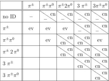
Table 2: The assignment of the various decay modes from the likelihood identification into classes analyzed by either m ^∗ _cn (cn) or m ^∗ _ev (ev). The row labeled ‘no ID’ combines the cones where no identification was possible with those identified as leptonic decays and all other channels not used in the analysis. τ → 3 π ^± ν τ includes τ → π ^± K ⁰ ν τ . For τ → π ^± ν τ versus τ → 3 π ^± ν τ see text.

The pseudomass used to analyze an event depends on its identified decay modes. This choice of method can either be m ^∗ _cn applied to one or both cones of the event independently or m ^∗ _ev applied to the whole event. Table 2 illustrates the association of the decay modes of the τ to the two methods. The association has been optimized to give the smallest possible statistical error on m τ , a process which results in decays with high hadronic masses typically being assigned to the m ^∗ _cn method, leaving the lighter hadronic masses for m ^∗ _ev . Every decay or event is only analyzed by one method to avoid statistical correlations.

A slightly more complicated procedure is used for events with a τ → 3 π ^± ν τ decay recoiling against a τ → π ^± ν τ . The 3-prong cone is initially subjected to the m ^∗ _cn method and the 1- prong cone neglected (see Tab. 2). If m ^∗ _cn turns out to be below the fit window described in the following section, the event is analyzed through m ^∗ _ev instead. This procedure could also be applied to other combinations of decay modes, but the gain in overall resolution is only marginal.

4

class method entries result in MeV

π ^± π ⁰ m ^∗ _cn 1467 1777.6 ± 7.2

π ^± 2 π ⁰ m ^∗ _cn 1311 1801.7 ± 12.6

3 π ^± m ^∗ _cn 2680 1776.1 ± 1.9

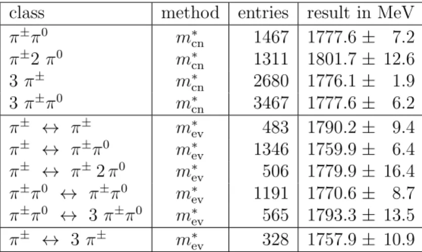
3 π ^± π ⁰ m ^∗ _cn 3467 1777.6 ± 6.2 π ^± ↔ π ^± m ^∗ _ev 483 1790.2 ± 9.4 π ^± ↔ π ^± π ⁰ m ^∗ _ev 1346 1759.9 ± 6.4 π ^± ↔ π ^± 2 π ⁰ m ^∗ _ev 506 1779.9 ± 16.4 π ^± π ⁰ ↔ π ^± π ⁰ m ^∗ _ev 1191 1770.6 ± 8.7 π ^± π ⁰ ↔ 3 π ^± π ⁰ m ^∗ _ev 565 1793.3 ± 13.5 π ^± ↔ 3 π ^± m ^∗ _ev 328 1757.9 ± 10.9

Table 3: The 10 classes of the analysis. The method applied, number of entries in the fit window, and a result (statistical error only) from a fit to each class alone are specified. The

‘π ^± ↔ 3 π ^± ’ class only contains those events not used in the ‘3 π ^± ’ class (see text).

In the following steps of the analysis the distributions of m ^∗ _cn are handled in exactly the same way as those of m ^∗ _ev . We define the following classes (see Tab. 2):

• Four classes corresponding to the decay modes τ → π ^± π ⁰ ν τ , τ → π ^± 2 π ⁰ ν τ , τ → 3 π ^± ν τ , and τ → 3 π ^± π ⁰ ν τ which are analyzed with the m ^∗ _cn method;

• Five classes for the different combinations of decay modes analyzed with the m ^∗ _ev method;

• One class for the τ → π ^± ν τ versus τ → 3 π ^± ν τ decays described in the previous para- graph.

Each class is further subdivided into subclasses according to the expected resolution. This avoids having information from well reconstructed entries degraded by the overlay of those entries with poorer resolution. There is a total of 25 subclasses, between one and five per class. The criteria used for the classification of the expected resolution is the quality of the reconstruction of the hadronic system, features like the presence of z-chamber or silicon hits on the tracks, the number and momentum of the reconstructed neutral pions, the probability of a vertex fit or the polar angle of the cone. The best resolution ⁵ in the pseudomass m ^∗ _cn of 17 MeV is achieved in the τ → 3 π ^± ν τ class, and this class also has the largest weight in the final result. For m ^∗ _ev , the best resolution is 21 MeV in the τ → π ^± ν τ versus τ → π ^± ν τ class.

Table 3 gives some more information on the classes. Figures 1 and 3 correspond to the subclass with the best resolution.

5

The resolution is defined as the r.m.s of the difference between true and reconstructed pseudomass from

simulated events that fall into the fit window.

4 Extraction of the τ Mass

The value of the τ mass is extracted from the pseudomass distribution by means of unbinned maximum likelihood fits. The distributions are parameterized by a step function multiplied by a polynomial of up to third order. For each subclass one of the following step functions is chosen, depending on which gives the best description of the data:

f (x) =



 

 

 

 

 

 

 

  1 2

1 − x

√ 1 + x ²

1 1 + e ^x 1 π

π

2 − arctan (x)

(2)

The variable x is related to the pseudomass by x = b i (a i + δ + m ^∗ ) where a i and b i are fit parameters and m ^∗ is the pseudomass, the measured quantity. The index i labels the sub- classes. The parameter δ is a common shift of all distributions. The order of the polynomial is increased from zero until a reasonably good parameterization of the distribution is achieved. ⁶ Only events in the vicinity of the cutoff are used for the fits. The upper end of the fitting window is 2 GeV for all subclasses. The values of the lower bound range from 1.4 to 1.6 GeV, depending on the subclass. For each subclass the lower bound is decreased from 1.6 GeV until no further significant reduction of the expected statistical error is observed. After the initial parameterization of the m ^∗ distributions, the fit windows are reduced by 50 MeV on each side to ensure a stable parameterization in all areas that might be reached in the course of the following fits. The type of step function, the order of the polynomial, and the size of the fitting window are determined for each subclass separately from a Monte Carlo simulation [6].

The functional dependence of the pseudomass distribution on m τ is very simple in the vicinity of the cutoff. In this region the shape of the distribution does not depend on m τ . On a variation of m τ the whole distribution is shifted along the pseudomass axis by an amount identical to the shift in m τ . We will use this relation to extract the result, although it is not strictly correct away from the cutoff. We have checked that the fit windows are small enough so as not to introduce a systematic bias from this procedure.

The τ mass is extracted in three steps. In the first step, the distributions from simulated events are fitted for each subclass separately in order to fix the parameters of the fit function, i.e. the position and width of the step function (a i , b i ), and the coefficients of the polynomials.

In the second step the same simulated distributions are simultaneously fitted using the slightly reduced fit window. A common shift δ _MC is the only free parameter in this fit with all other parameters fixed to the values obtained in the first step. In the third step, the same common fit is applied to the data, but with δ data as the free parameter. The result is calculated from m τ = m ^MC _τ + δ _data − δ _MC with m ^MC _τ = 1777 MeV the τ mass used in the simulation. The result is 1775.1 MeV with a statistical error of 0.4 MeV from the Monte Carlo and 1.6 MeV from the data. Results were also determined for each class separately as a cross check, the results are shown in table 3.

6

We histogram the data and apply a χ

test to decide on the quality of the description.

6

5 Systematic Uncertainties

The most significant contributions to the overall systematic uncertainty are described in this section.

• The dominant systematic uncertainty comes from the calibration of the tracking chambers and the electromagnetic calorimeter. We use muons and electrons of 45 GeV from Z ⁰ decays and Bhabha scattering to check these calibrations. We find uncertainties in the momentum scale of the tracking chambers relative to the Monte Carlo of 0.1 % and for the calorimeter of less than 0.3 %. Several different scenarios are employed to extrapolate these uncertainties to the momentum and energy ranges relevant to τ decays. The most pessimistic scenario, a scaling of 1/p T by a factor, gives a systematic error from the tracking of 900 keV. The uncertainty in the calibration of the calorimeter is found to have a negligible impact (250 keV), since it only effects channels with neutral pions.

• Uncertainties in modeling the resolution of the tracking chambers result in an error of 40 keV on the measurement of m τ . The resolution of the electromagnetic calorimeter has a negligible impact.

• In order to estimate the systematic error contribution from the modeling of the dynamics of the τ decays, we have varied the mass and width of the a 1 meson in the 3π ^± final state by ± 100 MeV and changed the fraction of ωπ events in the 4π final state by ± 20 %. The first two variations each change the result by 100 keV, while the third has a negligible impact. We also tested two different models for the τ → 3 π ^± ν τ decay [7]. Using these models the result changes by less than 100 keV.

• In the derivation of the pseudomass formulae the assumption E τ = E beam is used, which is only true in the absence of initial state radiation. Low energy photons from initial state radiation have only a negligible effect on the measurement, while a variation of ± 1 % of the rate of hard initial state radiation results in an uncertainty on the measurement of 70 keV.

• The uncertainty in the calibration of the beam energy of LEP has a negligible effect. An error of 2 MeV on the beam energy changes the result by less than ± 40 keV.

• The calculation of the pseudomasses assumes that the ν τ has zero mass. A value of 18.2 MeV, the current limit on the τ neutrino mass [8], increases the result by 110 keV.

No systematic error is assigned.

• Systematic uncertainties related to background from misidentified τ decays are negligible, since their pseudomass distributions show no significant structure in the region of the cutoff. Background from non-τ sources is also negligible.

• To address possible biases from the parameterization of the pseudomass distributions, we increased the lower edge of the window for all channels, in steps of 25 MeV, to 1.6 GeV.

Furthermore, we fitted the distributions with the type of step function giving the second best description of the data. Both studies showed consistent results.

Adding in quadrature all systematic uncertainties including the statistical error from the Monte

6 CPT Test

To test CPT invariance we compare the masses of the positively and negatively charged τ leptons. The pseudomass method m ^∗ _cn allows a separate measurement for the positive and the negative τ lepton, whereas the m ^∗ _ev method implicitly assumes the two masses to be identical and therefore the m ^∗ _cn method is used for all decays. The measurement does not use any Monte Carlo simulation which reduces the systematic uncertainties.

For the CPT analysis the m ^∗ _cn distributions are separated according to the net charges of the cones. To extract the result we use a procedure similar to the one used to measure m τ . In the first step, the distributions of the positive or negative τ leptons are fitted subclass by subclass to fix the parameterizations. Then all the distributions of the positive τ leptons are fitted simultaneously with the parameters fixed to the values from the first fit, allowing only for a common shift in mass δ ⁺ . Then negative τ leptons are fitted the same way with δ ⁻ as the free parameter. If CPT invariance is conserved, the two shifts must be equal. We obtain the result δ ⁺ − δ ⁻ = 0.0 ± 3.0 MeV.

In a τ pair event produced in e ⁺ e ⁻ collisions, a mass difference between the positive and negative τ will also create a difference in energy between the two τ. Although in principle this invalidates the assumption E τ = E beam , this effect is numerically negligible.

Most sources of systematic errors affect the result for the positive and negative lepton in the same way, so that their contributions cancel. The largest error in the mass difference comes from possible differences in the calibration between positively and negatively charged tracks which is limited to less than 0.2 % by studying muon pairs. This implies a systematic uncertainty on the mass difference of 1 MeV. All other systematic errors are negligible and the total systematic error is small compared to the statistical error. It is added in quadrature to the statistical error.

The m ^∗ _cn method uses the momentum and mass of the hadronic system measured from the curvature of the tracks in the magnetic field of the detector. These tracks originate mainly from pions with a small fraction coming from kaons. The charge and the charge to mass ratio of these particles have to be known in order to convert the observed curvature into a momentum measurement. However, without assuming CPT invariance, it is no longer obvious that the charge and mass are the same for positively and negatively charged pions ⁷ . Experimentally, the relative pion mass difference has been measured to be (2 ± 5) × 10 ^{− 4} which is below our sensitivity, but the pion charge difference has not been measured separately. However, the pion charges could be different due to a charge difference between the τ ⁺ and the τ ⁻ or because of charge non-conservation. A charge difference between π ⁺ and π ⁻ as large as 5 % would invalidate our measurement.

This is the first test of CPT invariance with τ leptons. The result is m ⁽ τ

⁾ − m ⁽ τ

⁾

m ( τ ) = (0.0 ± 1.8) × 10 ^{− 3} . (3)

where m(τ ) is the charge-independent result from the previous section. This result implies that the relative τ mass difference is smaller than 3.0 × 10 ^{− 3} at the 90 % confidence level.

7

A common deviation of the charge of positive and negative pion from the charge of the electron or the τ would not spoil the measurement. Only a difference between π

and π

is relevant.

8

7 Summary

We have measured the mass of the τ lepton from the pseudomass distributions of the hadronic τ decays recorded by the OPAL detector at LEP and obtained a result of

m τ = 1775.1 ± 1.6(stat.) ± 1.0(sys.) MeV (4) where the first error is statistical and the second systematic. The result is compared to other measurements in fig. 4. Using the pseudomass m ^∗ _cn we obtain an independent measurement of the mass of the positive and negative τ. The two numbers are consistent and a limit of 3.0 × 10 ^{− 3} on the relative mass difference is be placed at the 90 % confidence level. This is the first test of CPT invariance in τ physics.

1755 1760 1765 1770 1775 1780

ARGUS 1776.3 ±2.8 CLEO 1778.2 ± 1.4 BES 1776.96 ^+0.31 _–0.27 OPAL 1775.1 ±1.9

m _τ [MeV]

1755 1760 1765 1770 1775 1780

Figure 4: Comparison of our result with the results from ARGUS [1], CLEO [9], and BES [10].

The shaded band indicates the current world average [8], which does not include the OPAL result.

Acknowledgments

We particularly wish to thank the SL Division for the efficient operation of the LEP accelerator at all energies and for their continuing close cooperation with our experimental group. We thank our colleagues from CEA, DAPNIA/SPP, CE-Saclay for their efforts over the years on the time-of-flight and trigger systems which we continue to use. In addition to the support staff at our own institutions we are pleased to acknowledge the

Department of Energy, USA, National Science Foundation, USA,

Particle Physics and Astronomy Research Council, UK,

Natural Sciences and Engineering Research Council, Canada,

Minerva Gesellschaft,

Benoziyo Center for High Energy Physics,

Japanese Ministry of Education, Science and Culture (the Monbusho) and a grant under the Monbusho International Science Research Program,

Japanese Society for the Promotion of Science (JSPS), German Israeli Bi-national Science Foundation (GIF),

Bundesministerium f¨ ur Bildung und Forschung, Forschung und Technologie, Germany, National Research Council of Canada,

Research Corporation, USA,

Hungarian Foundation for Scientific Research, OTKA T-029328, T023793 and OTKA F-023259.

References

[1] ARGUS Collaboration, H. Albrecht et al. , Phys. Lett. B 292 (1992) 221.

[2] CLEO Collaboration, R. Ballest et al. , Phys. Rev. D 47 (1993) 3671.

[3] OPAL Collaboration, K. Ahmet et al. , Nucl. Instr. and Meth. A 305 (1991) 275;

P.P. Allport et al. , Nucl. Instr. and Meth. A 324 (1993) 34;

P.P. Allport et al. , Nucl. Instr. and Meth. A 346 (1994) 476.

[4] OPAL Collaboration, G. Alexander et al. , Phys. Lett. B 266 (1991) 201, OPAL Collaboration, R. Akers et al. , Phys. Lett. B 328 (1994) 207.

[5] OPAL Collaboration, J. Allison et al. , Z. Phys. C 66 (1995) 31;

OPAL Collaboration, K. Ackerstaff et al. , Eur. Phys. J. C 7 (1999) 571.

[6] KORALZ, Version 4.02, S. Jadach, B. F. L. Ward, and Z. W¸as, Comp. Phys. Comm. 79 (1994) 503.

TAUOLA, Version 2.5, S. Jadach, Z. W¸as, R. Decker, and J. H. K¨ uhn, Comp. Phys. Comm.

76 (1993) 361.

[7] J. H. K¨ uhn and A. Santamaria, Z. Phys. C 48 (1990) 445;

N. Isgur, C. Morningstar and C. Reader, Phys. Rev. D 39 (1989) 1357.

[8] Particle Data Group, C. Caso et al. , Euro. Phys. J. C 3 (1998) 1.

[9] CLEO Collaboration, A. Anastassov et al. , Phys. Rev. D 55 (1997) 2559, ibid. D 58 (1998) 119904.

[10] BES Collaboration, J.Z. Bai et al. , Phys. Rev. D 53 (1996) 20.

10