ATLAS NOTE

(1)

ATLAS NOTE

ATLAS-CONF-2013-31

March 11, 2013

Minor revision: March 17, 2013

Study of the spin properties of the Higgs-like boson in the H → WW⁽^∗⁾ → eνµνchannel with 21 fb⁻¹ of √

s = 8TeV data collected with the ATLAS detector

The ATLAS Collaboration

Abstract

Recently, the ATLAS collaboration reported the observation of a new neutral particle in the search for the Standard Model Higgs boson. The measured production rate of the new particle is consistent with the Standard Model Higgs boson if it has a mass of about 125 GeV.

This note reports on the compatibility of the observed excess in the H → WW^(∗) → eνµν search with either a spin-0 or a spin-2 particle with positive charge-parity. Analysis of the LHC collision data collected in 2012 with the ATLAS detector results in the exclusion of a benchmark spin-2 model at 95% confidence level, in favour of the Standard Model Higgs boson.

Revised bands on figure 13, no change in results with respect to the version of March 11, 2013

c

Reproduction of this article or parts of it is allowed as specified in the CC-BY-3.0 license.

(2)

1 Introduction

The observation of a new particle in the search for the Standard Model (SM) Higgs boson [1] is only the first step in understanding the nature of electroweak symmetry breaking, and much work remains to characterise its physical properties. This new particle is consistent with the prediction from the SM in terms of production rate in different search channels. The decay to pairs of vector bosons whose net electric charge is zero identifies the new particle as a neutral boson. The Landau-Yang-theorem forbids the decay of a spin-1 particle into a pair of photons [2, 3]; the spin-1 hypothesis is therefore strongly disfavoured by the observation in the diphoton channel. Studies of theH→ZZ→````process have excluded spin-parity states J^P = 0⁻ and J^P = 1⁺ at a 98% confidence level in favor of a SM Higgs boson [4]. This analysis aims at determining the spin of the Higgs-like boson assuming positive charge-parity, by studying theH→WW^(∗)→eνeµνµfinal states¹with no reconstructed high transverse momentum (p_T) jets. This channel is the most sensitive channel in the overall H → WW^(∗) → `ν`ν (` = e, µ) analysis [5]. Other channels are not expected to add much in terms of spin sensitivity due to the presence of large backgrounds which cannot be removed without greatly reducing the acceptance of the spin-2 model considered in this analysis.

The spin of the new particle will manifest itself in the angular decay characteristics and the momenta of the decay particles [6]. The decay H → `ν`νprovides a relatively large signal yield, which allows for a shape analysis of kinematic distributions despite the poor invariant mass resolution due to the two unobserved neutrinos in the events.

The study presented in this note uses √

s = 8 TeV proton-proton collision data corresponding to an integrated luminosity of 20.7 fb⁻¹, collected with the ATLAS detector in 2012. Two hypotheses are tested against the observed excess of events in theH→WW^(∗) →`ν`νsearch (previously documented in Ref. [1]), namely a SM Higgs boson with J^P = 0⁺, from now on referred to as 0⁺, and a generic J^P = 2⁺_mgraviton-like tensor with minimal couplings [7], from now on referred to as 2⁺_m, as explained in Section 2. In that section a summary of the Monte Carlo (MC) simulation and data samples is also presented. Discriminating variables for spin determination in the H → WW^(∗) → eνµν channel are described in Section 3. The selections that define the data sample used in this analysis are presented in Section 4, followed by an investigation into the agreement between data and MC simulations in Section 5.

The spin analysis is based on a multivariate classifier known as a boosted decision tree (BDT), which is described in Section 6. The impact of systematic uncertainties on the determination is investigated in Section 7. Finally, the fitting procedure and results are presented in Section 8.

2 Data and simulated samples

The data used for this analysis were collected in 2012 using the ATLAS detector, a multi-purpose particle physics experiment with a forward-backward symmetric cylindrical geometry and near 4πcoverage in solid angle [8]. ATLAS consists of an inner tracking detector surrounded by a thin superconducting solenoid, electromagnetic and hadronic calorimeters, and an external muon spectrometer incorporating large superconducting air-core toroid magnets. The combination of these systems provides charged particle measurements together with efficient and precise lepton measurements over the pseudo-rapidity² range|η|< 2.5. Jets are reconstructed over the full coverage of the calorimeters,|η| < 4.9. This nearly- hermetic calorimetry coverage also provides a precise measurement of the missing transverse energy

1For simplicity, the notation used for particles and anti-particles is the same.

2ATLAS uses a right-handed coordinate system with its origin at the nominal interaction point (IP) in the centre of the detector, and thez-axis along the beam line. Thex-axis points from the IP to the centre of the LHC ring, and they-axis points upwards. Cylindrical coordinates (r, φ) are used in the transverse plane,φbeing the azimuthal angle around the beam line. The pseudo-rapidity is defined in terms of the polar angleθasη=−ln tan(θ/2).

(3)

(E^miss_T ).

Data were selected using inclusive single-muon and single-electron triggers. The two main triggers require the transverse momentum, p_T, of the lepton to exceed 24 GeV and that the lepton be isolated from nearby tracks.

In this analysis, the SM signal contribution includes only the dominant gluon fusion (ggF) production process. Thet¯tHand associated production mechanisms are negligible due to their much smaller cross sections, and thus are not considered. Since the analysis is only performed using events with no high pT

jets, the vector boson fusion process is also negligible.

For the J^P = 2⁺ signal, the most general amplitude of the decay into two identical vector bosons contains 10 different terms and 10 effective coupling constantsg_1..10which are in general complex numbers [7]:

A(H→VV)= Λ⁻¹

2g₁t_µνf^∗1,µαf^∗2,να+2g₂t_µνq_αq_β

Λ² f^∗1,µαf^∗2,νβ +g₃q˜^βq˜^α

Λ² t_βν(f^∗1,µνf_µα^∗2+ f^∗2,µνf_µα^∗1)+g₄q˜^νq˜^µ

Λ² t_µνf^∗1,αβf_αβ^∗(2) +m²_V 2g₅t_µν₁^∗µ₂^∗ν+2g₆q˜^µq_α

Λ² t_µν(₁^∗ν₂^∗α−₁^∗α₂^∗ν)+g₇q˜^µq˜^ν Λ² t_µν₁^∗₂^∗

!

+g₈q˜_µq˜_ν

Λ² t_µνf^∗1,αβf˜_αβ^∗(2)+g₉t_µαq˜^αµνρσ₁^∗ν₂^∗ρq^σ +g₁₀t_µαq˜^α

Λ² _µνρσq^ρq˜^σ(₁^∗ν(q₂^∗)+₂^∗ν(q₁^∗))

#

, (1)

whereq,q₁ andq₂ denote the 4-momenta of the spin-2 particle and of vector bosons, respectively, and

˜

q=q₁−q₂. The field strength tensor of the gauge boson with momentumqiand polarisationiis denoted f^(i),µν. The resonance wave function is given by a symmetric traceless tensort_µνandΛis the mass scale associated with physics beyond the Standard Model.

The large number of free parameters in the couplings of a spin-2 particle makes it very difficult to exclude a generic spin-2 model. Instead, in this analysis a simple model is tested, namely a graviton- like tensor with minimal couplings, 2⁺_m, where the only non-vanishing constants areg₁ = g₅ = 1. Two different production processes,qq → Handgg → H, are included for the 2⁺_mmodel, with an arbitrary defaultqqfraction, f_q_q_¯ = 25%. As will be discussed later, the analysis is performed for various values of fqq¯. Due to the lack of a definite prediction for the production cross section for 2⁺_mevents, the overall yield (proportional to cross section times branching ratio) of the signal events is fitted directly from the observed data.

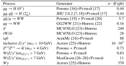
The Monte Carlo generators used to model signal and background processes are listed in Table 1 and further details can be found in Ref. [5]. The p_T spectrum for the 0⁺ggF production in Powheg[9] is weighted to agree with the prediction from HqT [10]. Heavy quark mass effects in the ggF production are also included [11]. For the decay of the new particle (either 0⁺or 2⁺_m), only theH→WW⁽^∗⁾→eνµν decay channel is considered, including the small contributions from leptonicτdecays.

In all the MC simulations, the CT10 PDF set [12] is used for the Powhegand MC@NLO samples, and CTEQ6L1 [13] is used for the Alpgen, MadGraph, and Pythia8 samples. Acceptances and efficiencies are obtained from a full simulation [14] of the ATLAS detector using Geant4 [15]. The simulation incorporates a model of the event pile-up conditions in the 2012 data, including both the effects of multiple pp collisions in the same bunch crossing (“in-time” pile-up) and in nearby bunch crossings (“out-of-time” pile-up).

(4)

Process Generator σ· B(pb) gg→H(0⁺) Powheg[16]+Pythia8 [17] 0.44 gg,qq→H(2⁺_m) JHU 2.0.2 [7, 18]+Pythia8 [17] 0.44 qq/g¯ →WW Powheg[19]+Pythia6 [20] 5.7

gg→WW GG2WW [21]+Herwig[22] 0.16

tt¯ MC@NLO [23]+Herwig 240

tW/tb MC@NLO [23]+Herwig 28

tqb AcerMc[24]+Pythia6 88

inclusiveZ/γ^∗(m``>10 GeV) Alpgen[25]+Herwig 16·10³ Z^(∗)Z^(∗)→4l(m``>4 GeV) Powheg+Pythia8 0.73 W(Z/γ^∗)(m(Z/γ^∗)>7 GeV) Powheg+Pythia8 0.83 W(Z/γ^∗)(m(Z/γ^∗)<7 GeV) MadGraph[26–28]+Pythia6 11

Wγ Alpgen[25]+Herwig 370

Table 1: Monte Carlo generators used to model the signal and background processes, and the corresponding cross sections at √

s = 8 TeV (given m_H = 125 GeV in the case of the signal processes).

Leptonic decays of W/Z bosons are always assumed. The quoted cross sections include the branching ratios and are summed over lepton flavours (third column) [9,29]. The exception is top quark production, for which inclusive cross sections are quoted.

3 Spin-sensitive variables

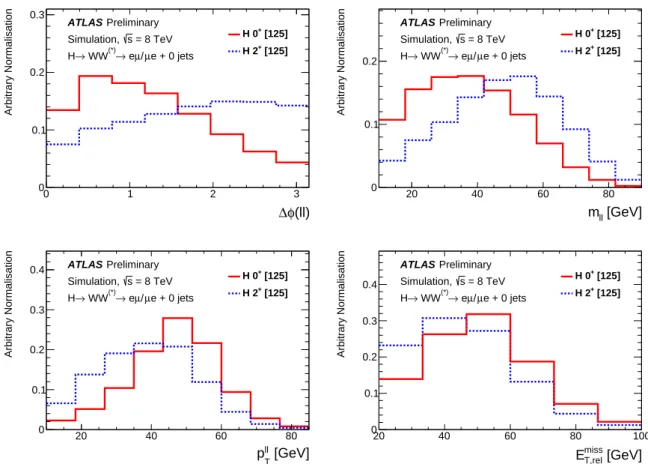
Spin correlations between the decay products affectH → WW^(∗) → `ν`νevent topologies by shaping angular distributions of the leptons as well as the lepton momenta and missing transverse energy. Two of the most sensitive variables for measuring spin are the dilepton invariant mass,m_``, and the azimuthal separation of the two leptons,∆φ``. In addition to these variables, 0⁺and 2⁺_m have markedly different E^miss_T,rel spectra³, and different distributions of the dilepton transverse momentum,p^``_T. Distributions of all these quantities for 0⁺and 2⁺_m particles are shown in Fig. 1 for signal events withE^miss_T > 20 GeV, no jets, and two opposite-charge leptons. At this level of selection there are clear differences in the shapes of the variables. As will be seen, this motivates a different set of selection criteria compared to the rate measurement [5], which is optimised for a 0⁺ signal. However, in order to reduce the background contributions, further selections are applied which dilute the differences between 0⁺and 2⁺_mparticles.

4 Event selection

Collision events with reconstructed leptons within |η| < 2.5 are selected using lepton identification criteria identical to the production rate measurement [5]. AH →WW^(∗) →`ν`νcandidate sample is then selected by requiring two opposite-charge leptons, with no additional leptons above p_T >15 GeV in the event. The leading lepton is required to have p_T > 25 GeV and the sub-leading leptonp_T >15 GeV. At least one of the lepton candidates must match a trigger object. Only events with different flavour leptons (eµorµe, where the order indicates which lepton has largerp_T) are selected.

There are three major sources of background after the dilepton selection cuts, namely inclusiveZ/γ^∗ (referred to as Drell-Yan), diboson, and top quark (t¯tand single top) production processes. W bosons produced in association with hadronic jets can also be a large source of background if a jet is misidentified as a lepton, but the requirement of two high-pT, isolated leptons greatly reduces the background sources

3E^miss_T,rel ≡ E^miss_T ·sin∆φ, where∆φ is the azimuthal separation between missing transverse energyE^miss_T and the nearest reconstructed object (lepton or jet withpT>25 GeV) or ^π₂radians, whichever is smaller.

(5)

φ(ll)

∆

0 1 2 3

Arbitrary Normalisation

0 0.1 0.2

0.3 ATLAS Preliminary

= 8 TeV s Simulation,

e + 0 jets µ µ/

→ e WW(*)

→ H

[125]

H 0+

[125]

H 2+

[GeV]

mll

20 40 60 80

0 0.1 0.2

Preliminary ATLAS

e + 0 jets µ µ/

→ e WW(*)

→ H

[125]

H 0+

[125]

H 2+

[GeV]

ll

pT

20 40 60 80

0 0.1 0.2 0.3

0.4 ATLAS Preliminary = 8 TeV s Simulation,

e + 0 jets µ µ/

→ e WW(*)

→ H

[125]

H 0+

[125]

H 2+

[GeV]

miss T,rel

E

20 40 60 80 100

0 0.1 0.2 0.3 0.4

e + 0 jets µ µ/

→ e WW(*)

→ H

[125]

H 0+

[125]

H 2+

Figure 1: Distributions of (starting from upper left)∆φ_``,m_``, p^``_T, andE^miss_T,relforJ^P=0⁺(solid red line) and 2⁺_m(dashed blue line) events with two opposite-charge leptons,E^miss_T > 20 GeV, and zero jets. The definitions of these quantities are discussed in the text. The distributions are normalised to unit area.

from fake leptons.

The main Drell-Yan contribution is comprised ofZ → ττ → ``+E^miss_T events. This contribution can be suppressed by requiringE^miss_T,relabove 20 GeV, becauseE_T,rel^missstill tends to be small in these events, owing to the fact that the neutrinos from the τdecays are usually back-to-back. The background in- volving top quarks is suppressed by vetoing events containing jets with p_T > 25 GeV and|η| < 4.5, as reconstructed using the anti-kt algorithm [30] with distance parameterR = 0.4. The jet p_T threshold is increased to 30 GeV in the forward region 2.5<|η|<4.5 to reduce the inefficiency of the jet veto arising from jets produced by pile-up. The lepton selection, E_T,rel^miss and jet veto cuts comprise a set that will be referred to as “pre-selection cuts” in the following text.

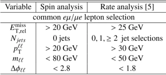
Further lepton topology cuts are then applied to optimise sensitivity for both 0⁺ and 2⁺_m signals simultaneously, namely on the transverse momentum of the dilepton system, p^``_T > 20 GeV, on the invariant mass,m_`` <80 GeV, and on the azimuthal angular difference between the leptons,∆φ`` <2.8 radians. These cuts significantly reduce the amount ofWW continuum and Drell-Yan background. The combination of all of these cuts defines a sample enriched with both 0⁺ and 2⁺_m events. These lepton topology selections are looser than those used in the rate measurement, which assumes a SM scalar Higgs boson. A comparison of the selection for the spin measurement to that used in theH →WW^(∗) →`ν`ν rate measurement is shown in Table 2. This set of cuts will be referred to as “signal region cuts” in the following text.

(6)

Variable Spin analysis Rate analysis [5]

commoneµ/µelepton selection E^miss_T,rel >20 GeV >25 GeV N_jets 0 jets 0,1,≥2 jet selections

p^``_T >20 GeV >30 GeV m_`` <80 GeV <50 GeV

∆φ`` <2.8 <1.8

Table 2: List of selection cuts applied for the H → WW^(∗) → `ν`νspin (left column) and rate (right column) measurements, after the common dilepton selections.

5 Backgrounds

The main background for this analysis after all the topological selection cuts is the SM production of WW pairs followed by smaller backgrounds fromt¯t, single top (tW, tb andtqb),W+jets, Z+jets and WZ/ZZ/Wγ processes. The contributions predicted by MC fromWW, top quark andZ+jets processes are normalised to observed rates in control regions dominated by the relevant background source. The W+jets background is fully estimated from data. The shapes and normalisations of non-WW diboson backgrounds are estimated using simulation and cross-checked in a validation region [5]. The control and validation regions are defined by selections similar to those used in the signal region but with some criteria reversed or modified to obtain signal-depleted samples enriched in a particular background.

The correlations introduced among the different background sources by the presence of other processes in the control regions are fully incorporated in the statistical procedure to test the compatibility between data and the two spin hypotheses as described in Section 8.1. In the following, each background estimate is described after any others on which it depends.

5.1 W+jets background

The W+jets background contribution is estimated using a control sample of events in which one of the two leptons satisfies the identification and isolation criteria required for the signal selection [5], and the other lepton (denoted “anti-identified”) fails these criteria but satisfies a loosened selection. The dominant contribution to this background comes fromW+jets events in which a jet produces an object which is reconstructed as a lepton.

TheW+jets background in the signal region is obtained by scaling the number of events in the data control region by a fake factor. The fake factor is defined as the ratio of the number of fully identified lepton candidates passing all selections to the number that are anti-identified. It is estimated as a function of the anti-identified leptonp_T and using an inclusive dijet data sample.

The uncertainty on the lepton fake factor is the main uncertainty on theW+jets background estimation. It is dominated by differences in jet composition between dijet andW+jets samples as observed in MC simulation. The total relative uncertainty on this background is 45% for mis-identified electrons and 40% for mis-identified muons. This systematic uncertainty is treated as uncorrelated between electrons and muons, reducing the effective uncertainty on the totalW+jets background.

5.2 Z/γ^∗→ ττcontrol sample

TheZ/γ^∗→ττbackground is the dominant source ofZ+jets events in the different lepton flavour channel. In the signal region its contribution is of the same order as theW+jets contribution. In the control

(7)

Events

0 2000 4000 6000 8000 10000 12000 14000 16000 18000 20000 22000 24000

Data SM (sys ⊕ stat)

WW WZ/ZZ/Wγ

t

t Single Top

Z+jets W+jets [125]

H 0+

ATLAS Preliminary

Ldt = 20.7 fb-1

∫

= 8 TeV, s

ν νe µ ν/ µ ν

→e WW(*)

→ H

Njets

0 1 2 3 4 5 6 7

Data / SM 0.6

0.81 1.2 1.4

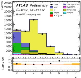
Figure 2: Distribution of number of jets after theE^miss_T,relcut. The lepton flavours are combined. The shaded area represents the uncertainty on the signal and background yields from statistical, experimental, and theoretical sources.

region defined by m_`` < 80 GeV and ∆φ`` > 2.8, in addition to the pre-selection, a Z/γ^∗ → ττpu- rity of more than 90% is expected, as obtained from MC samples. Residual contamination from other backgrounds is subtracted from the data, using simulation and theW+jets estimate from data. The normalisation factor, used to scale the Drell-Yan prediction from simulation, is then obtained from the ratio of the number of events in data, with backgrounds not originating fromZ/γ^∗subtracted, and the number of MC events inZ/γ^∗→ττ. The normalisation factor is 0.92±0.02 (stat). The total uncertainty on the estimate is 8%, which includes both statistical and systematic uncertainties as described in Section 7.

5.3 Top-quark control sample

The number of background events from top quark production in the signal region is normalised to the number of events satisfying modified pre-selection criteria, namely, the selection up to but not including the jet veto. This sample is dominated by top quark events, as shown in Fig. 2. The small contribution of non-top backgrounds to this sample is estimated from simulation except for theW+jets contribution, which is estimated from data. The fraction of top events that survive the jet veto is then estimated in data using a control sample with at least one b-tagged jet, as described in Ref. [5]. The efficiency for the remaining requirements on p^``_T, m_``, and∆φ`` is taken from simulation. The ratio of the resulting prediction to the one from simulation alone is 1.07±0.03 (stat). The total uncertainty on the estimate is 14%, which includes both statistical and systematic uncertainties as described in Section 7. The dominant systematic uncertainty is due to renormalisation and factorisation scale uncertainties.

5.4 WW control sample

The MC prediction for theWW background is normalised using a control region defined with the same selection as the signal region except that the∆φ_``requirement is removed and the upper bound onm_``is replaced with a lower bound,m_``> 80 GeV. Events fromWW contribute about 70% of the total events in this control region. Contributions from sources other thanWW are derived as they are for the signal region, including the top,Z/γ^∗→ττandW+jets backgrounds. The resultingWW normalisation factor applied to the MC prediction is 1.08±0.03, including only the statistical uncertainty. The total uncertainty

(8)

0⁺ 2⁺_m WW WZ/ZZ/Wγ t¯t tW/tb/tqb Z+jets W+jets Total Bkg. Observed jet veto 180±2 130±2 5080±20 420±20 540±10 330±10 4180±40 580±10 11130±50 11493 pT,``>20 GeV 170±1 120±1 4620±20 380±10 520±10 310±10 670±20 460±10 6950±40 7261 m``<80 GeV 170±1 120±1 2210±20 230±10 180±10 120±10 610±20 300±10 3660±30 3964

∆φ``<2.8 170±1 110±1 2190±20 230±10 180±10 120±10 290±20 280±10 3280±20 3615 Z→ττcontrol region 4±1 9±1 100±10 10±1 5±1 3±1 3530±40 100±10 3740±40 3474 WWcontrol region 1±1 2±1 2230±10 150±10 340±10 190±10 60±7 150±10 3110±20 3297

Table 3: The expected numbers of signal (mH =125 GeV) and background events after the requirements listed in the first column, as well as the observed number of events, are shown for the signal region (upper part) along with the control regions for Z/γ^∗ → ττ(middle part) andWW (lower part). The W+jets background is estimated entirely from data, whereas MC predictions normalised to data in control regions are used for theWW, top andZ/γ^∗→ττprocesses. The signal for both spin hypotheses is scaled to the prediction from the SM for a 0⁺ Higgs boson. For the 2⁺_msample aqq¯ fraction of fqq¯ = 25% is used.

Only statistical uncertainties associated with the numbers of events in the MC samples are shown. The yields in this table for theZ/γ^∗→ττandWW control regions are not normalised to the data. However, appropriate normalisation factors are applied to the yields in the signal region.

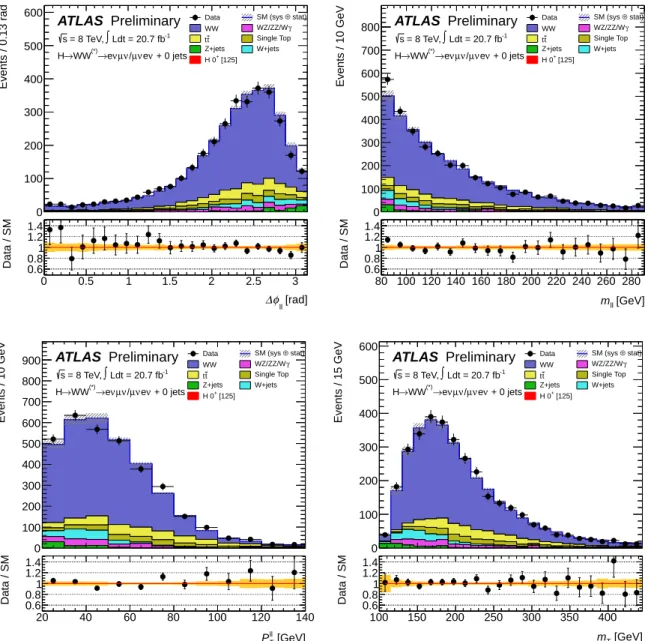
on the predicted WW background in the signal region, including both statistical and systematic effects (described in Section 7) on the yield in the control region and the extrapolation to the signal region, is 10%. Validation of the kinematic distributions, especiallym_``, p^``_T,∆φ_`` and the transverse massm_T in theWW control region, as shown in Figure 3, demonstrates that this background is well-modelled. The transverse massm_Tis defined as

m_T= q

(E^``_T +E_T^miss)²− |p^``_T +E^miss_T |², whereE_T^``= q

|p^``_T|²+m²_``. 5.5 Event yield

The expected numbers of signal and background events at several stages of this selection are presented in Table 3. The rightmost column shows the observed numbers of events in the data. The uncertainties shown for the various background contributions, as predicted from simulation, include only the statistical uncertainties. The excess of data events over the total expected background events is compatible with the observation of the new particle atm_H = 125 GeV [5]. The differences between the observed and the expected events in the control regions are taken into account in the normalisation factors applied to the MC predictions in the signal region. These normalisation factors are applied in all of the following figures.

6 Analysis method

The 0⁺ and 2⁺_mhypotheses are tested using a two-dimensional kinematic shape fit. The discriminants used in the fit are outputs of two different boosted decision trees (BDT), trained separately against all backgrounds to identify 0⁺and 2⁺_mevents, respectively. The BDT for 2⁺_mevents is retrained for each f_q¯_q fraction.

A decision tree is a collection of cuts designed to classify events as signal-like or background-like.

Using cuts on a chosen set of discriminant variables, the events from a training sample of signal and background events are successively split to form a binary tree structure. At this point the tree contains many terminal nodes, each having predominantly signal or background events. A given signal event is correctly identified if it is in a signal-dominated leaf, and vice-versa for background events. Another tree

(9)

Events / 0.13 rad

0 100 200 300 400 500

600 _Data _{SM (sys}_⊕_stat)

WW WZ/ZZ/Wγ

t

t Single Top

Z+jets W+jets [125]

H 0+

Ldt = 20.7 fb-1

∫

= 8 TeV, s

+ 0 jets ν νe µ ν/ µ ν

→e WW(*)

→ H

[rad]

φll

∆

0 0.5 1 1.5 2 2.5 3

Data / SM 0.60.8

1 1.2 1.4

Events / 10 GeV

0 100 200 300 400 500 600 700 800

Data SM (sys ⊕ stat)

WW WZ/ZZ/Wγ

t

t Single Top

Z+jets W+jets [125]

H 0+

Ldt = 20.7 fb-1

∫

= 8 TeV, s

→e WW(*)

→ H

[GeV]

mll

80 100 120 140 160 180 200 220 240 260 280

Data / SM 0.60.8

1 1.2 1.4

Events / 10 GeV

0 100 200 300 400 500 600 700 800

900 ^Data_WW ^{SM (sys} WZ/ZZ/W^⊕γ^stat)

t

t Single Top

Z+jets W+jets [125]

H 0+

Ldt = 20.7 fb-1

∫

= 8 TeV, s

→e WW(*)

→ H

[GeV]

ll

PT

20 40 60 80 100 120 140

Data / SM 0.6

0.8 1 1.2 1.4

Events / 15 GeV

0 100 200 300 400 500

600 Data SM (sys ⊕ stat)

WW WZ/ZZ/Wγ

t

t Single Top

Z+jets W+jets [125]

H 0+

Ldt = 20.7 fb-1

∫

= 8 TeV, s

→e WW(*)

→ H

[GeV]

mT

100 150 200 250 300 350 400

Data / SM 0.6

0.8 1 1.2 1.4

Figure 3: ∆φ_``, m_``, p^``_T andm_T distributions in theWW control region. The lepton flavourse/µand µ/e are combined. The negligible signal shown is formH = 125 GeV. The shaded area represents the uncertainty on the signal and background yields from statistical, experimental, and theoretical sources.

The 0⁺signal is too small to see in these distributions.

(10)

is grown to better separate the signal and background events that were misidentified by the first tree. This proceeds iteratively until there is a collection of a specified number of trees. A weighted average is taken from all these trees to form a BDT output discriminant with values ranging between -1 and 1.

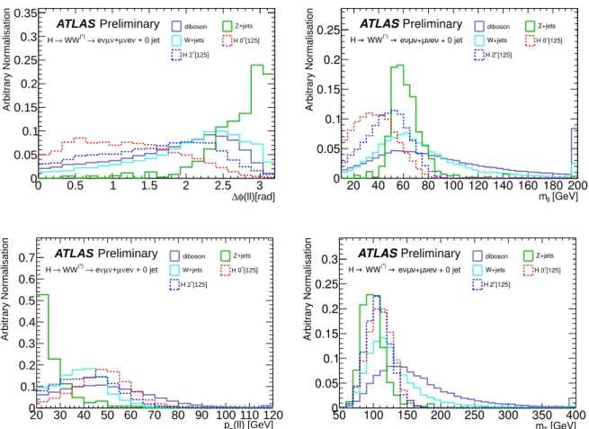
In this analysis, the BDT implementation in TMVAv4.1.3 [31] is used. Four discriminating variables are used in the BDT classifiers, namelym_``, p^``_T,∆φ`` andm_T. The first three variables simultaneously have very good separation power between both signals and all backgrounds and between the 0⁺and 2⁺_m hypotheses, as shown in Figures 1 and 4. The transverse mass provides a good separation for both 0⁺ and 2⁺_msignals from the top andWW backgrounds.

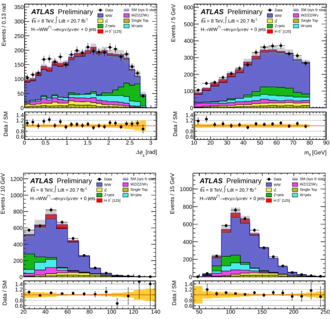
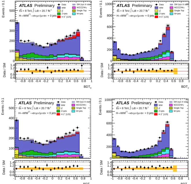
The BDT is trained using a looser event selection, namely after p^``_T > 20 GeV andm_`` < 100 GeV cuts. This looser selection has no impact on the final BDT performance in the signal region, and is utilised to reduce the statistical fluctuations, e.g. in theZ+jets sample used in the training. Two separate BDT classifiers are developed: one classifier using a 0⁺ sample as signal and a second classifier using a 2⁺_m sample. The BDT outputs will be referred to as BDT₀ and BDT₂, respectively. The resultant BDT responses for 0⁺ and 2⁺_m training configurations are shown in Figure 5 for signal and background MC samples. One can see that BDT₂ has less discrimination power than BDT₀. This is because the angular distributions of the leptons for a 2⁺_msignal are more background-like. However, the correlation ofBDT₀andBDT₂in the 2D fit provides improved sensitivity compared to usingBDT₀alone. Further, as will be discussed in Section 7,BDT₂is sensitive to the f_q¯qassumption for the 2⁺_msignal, and therefore can be optimised specifically for different f_q¯q values. Figure 6 shows the distribution of the four BDT training variables in the signal region. The data distributions agree well with the MC prediction if the expected SM 0⁺signal is included in the prediction.

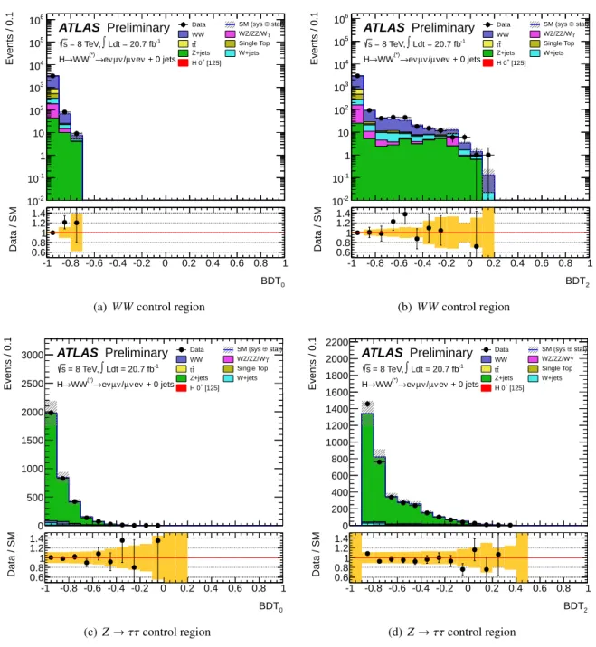
Background processes used in training both classifiers includeWW,t¯tand single top, as well asWZ, ZZ, Wγ, Wγ^∗, W+jets and Z + jets. Each background contribution is weighted by its corresponding cross section. The BDT output discriminant for both classifiers is calculated for each event in the signal and the control samples. Distributions of BDT₀andBDT₂for signal and background processes are shown in Figure 7 for the Z/γ^∗ → ττandWW control regions and in Figure 8 for the signal region.

The background BDT output distributions tend to peak at low values, while the signal output distributions typically peak at high values. The BDT output distributions are well modelled by the simulation.

The resultant two dimensional distribution of both classifiers is then used to test compatibility with the presence of a 0⁺or 2⁺_mparticle in the data.

The BDTs used in this analysis make use of the correlations between the input variables and therefore rely on a good description of these variables and of their correlations. Detailed studies have shown good agreement between data and MC for each input variable and for the correlation coefficients between the different variables. In addition, dedicated studies have been performed to verify that a BDT with the same four input variables can be trained to provide good separation between each of the main SM processes and the others in the background-enriched control regions described above.

7 Systematic uncertainties

The systematic uncertainties relevant for this measurement can be divided into two categories: experimental uncertainties affecting individual objects in the event, and theoretical uncertainties such as the estimation of the effect of higher-order terms through variations of the QCD scale inputs to Monte Carlo calculations. Especially important is the description of the dominantWW background both in terms of normalisation and shape, and also the modelling of the signal.

(11)

(ll)[rad]

φ

0 0.5 1 1.5 2 2.5∆ 3

0 0.05 0.1 0.15 0.2 0.25 0.3 0.35

diboson Z+jets W+jets H 0⁺[125]

[125]

H 2+

+ 0 jet ν νe µ ν+ µ ν

→ e WW(*)

→ H

[GeV]

mll

20 40 60 80 100 120 140 160 180 200

ArbitraryNormalisation

0 0.05 0.1 0.15

0.2

0.25 ^diboson ^Z+jets

W+jets H 0⁺[125]

[125]

H 2+

Preliminary ATLAS

+ 0 jet eν ν +µ ν µ eν

(*)→ WW H→

(ll) [GeV]

pT

20 30 40 50 60 70 80 90 100 110 120

0 0.1 0.2 0.3 0.4 0.5 0.6

W+jets H 0⁺[125]

[125]

H 2+

→ e WW(*)

→ H

[GeV]

mT

50 100 150 200 250 300 350 400

ArbitraryNormalisation

0 0.05 0.1 0.15

0.2 0.25

W+jets H 0⁺[125]

[125]

H 2+

Preliminary ATLAS

+ 0 jet eν ν +µ ν µ eν

(*)→ WW H→

Figure 4: ∆φ_``, m_``, p^``_T andm_T distributions after the pre-selection and p^``_T cuts. The lepton flavours are combined. The signal is shown for 0⁺and 2⁺_mhypotheses at m_H = 125 GeV. The distributions are normalised to unit area.

BDT0

-1 -0.8 -0.6 -0.4 -0.2 0 0.2 0.4 0.6 0.8 1

0 0.05 0.1 0.15 0.2 0.25 0.3 0.35 0.4

backgrounds [125]

H 0+ H 2⁺[125]

→ e WW(*)

→ H

BDT2

-1 -0.8 -0.6 -0.4 -0.2 0 0.2 0.4 0.6 0.8 1

0 0.05 0.1 0.15

0.2 0.25 0.3 0.35

0.4 backgrounds

[125]

H 0+ H 2⁺[125]

→ e WW(*)

→ H

Figure 5: BDT output distributions in the signal region, showing the shape differences between the 0⁺ and 2⁺_msignals and the backgrounds, for the BDT trained with 0⁺signal (left) and trained with 2⁺_msignal (right). The distributions are normalised to unit area.