Technical Report Series Center for Data and Simulation Science

Technical Report Series

Center for Data and Simulation Science

Niklas Wintermeyer, Andrew R. Winters, Gregor J. Gassner, Timothy War- burton

An entropy stable discontinuous Galerkin method for the shallow water equations on curvilinear meshes with wet/dry fronts acceler- ated by GPUs

Technical Report ID: CDS-2018-4

Available at http://kups.ub.uni-koeln.de/id/eprint/8656

Submitted on October 2, 2018

An entropy stable discontinuous Galerkin method for the shallow water equations on curvilinear meshes with wet/dry fronts accelerated by GPUs

Niklas Wintermeyer^a,ú, Andrew R. Winters^a, Gregor J. Gassner^a, Timothy Warburton^b

aMathematisches Institut, Universit¨at zu K¨oln, Weyertal 86-90, 50931 K¨oln

bDepartment of Mathematics, Virginia Tech, 225 Stanger Street, Blacksburg, VA 24061-0123

Abstract

We extend the entropy stable high order nodal discontinuous Galerkin spectral element approximation for the non-linear two dimensional shallow water equations presented by Wintermeyer et al. [N. Wintermeyer, A. R.

Winters, G. J. Gassner, and D. A. Kopriva. An entropy stable nodal discontinuous Galerkin method for the two dimensional shallow water equations on unstructured curvilinear meshes with discontinuous bathymetry.

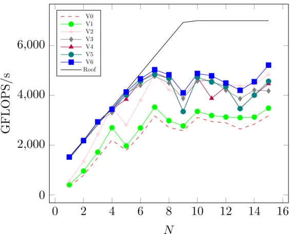
Journal of Computational Physics, 340:200-242, 2017] with a shock capturing technique and a positivity preservation capability to handle dry areas. The scheme preserves the entropy inequality, is well-balanced and works on unstructured, possibly curved, quadrilateral meshes. For the shock capturing, we introduce an artificial viscosity to the equations and prove that the numerical scheme remains entropy stable. We add a positivity preserving limiter to guarantee non-negative water heights as long as the mean water height is non-negative. We prove that non-negative mean water heights are guaranteed under a certain additional time step restriction for the entropy stable numerical interface flux. We implement the method on GPU architectures using the abstract language OCCA, a unified approach to multi-threading languages. We show that the entropy stable scheme is well suited to GPUs as the necessary extra calculations do not negatively impact the runtime up to reasonably high polynomial degrees (around N = 7). We provide numerical examples that challenge the shock capturing and positivity properties of our scheme to verify our theoretical findings.

Keywords: Shallow water equations, Discontinuous Galerkin spectral element method, Shock capturing, Positivity preservation, GPUs, OCCA

1. Introduction

The shallow water equations including a non-constant bottom topography are a system of hyperbolic balance laws

ht+ (hu)x+ (hv)y= 0, (hu)t+3

hu²+1 2g h²

4

x

+ (huv)y=≠ghbx, (hv)t+ (huv)x+3

hv²+1 2g h²

4

y

=≠ghby,

(1.1)

that are useful to model fluid flows in lakes, rivers, oceans or near coastlines, e.g [3, 28, 45]. We compactly write the system (1.1) as

˛

wt+Ò·(f,˛˛g)^T =S˛, (1.2)

úCorresponding author

Email address: nwinterm@math.uni-koeln.de(Niklas Wintermeyer)

with w˛ = (h, hu, hv)^T, f˛ = (hu, hu²+ ¹₂gh², huv)^T and ˛g = (hv, huv, hv² + ¹₂gh²)^T and source term S˛ = (0,≠ghbx,≠ghby)^T. The water height is denoted by h=h(x, y, t) and is measured from the bottom topographyb=b(x, y). The total water height is thereforeH =h+b. The fluid velocities areu=u(x, y, t) and v = v(x, y, t). An important steady state solution of (1.1) is the preservation of a flat lake with no velocity, the so-called “lake at rest” condition

h+b= const,

u=v= 0. (1.3)

A numerical scheme that preserves non-trivial steady state solutions, such as the “lake at rest” problem, is well-balanced, e.g. [17, 32]. Methods that are not well-balanced can produce spurious waves in the magnitude of the mesh size truncation error which pollutes the solution quality. This is particularly problematic because many interesting shallow water phenomena can be interpreted as perturbations from the lake at rest condition [26].

Due to the non-linear nature of the shallow water equations (1.1), discontinuous solutions may develop regardless of the smoothness of the initial conditions. Therefore, solutions to the PDEs (1.1) are sought in the weak sense. Unfortunately, weak solutions are non-unique and additional admissibility criteria are required to extract the physically relevant solution from the family of weak solutions. One important criteria for physically relevant solutions is the second law of thermodynamics, which guarantees that the entropy of a physical system increases as the fluid evolves. In mathematics, a suitable strongly convex entropy function can be used to ensure a numerical approximation obeys the laws of thermodynamics discretely [43]. A numerical scheme that satisfies the second law of thermodynamics is said to be entropy stable. Due to convention, the sign of the mathematical entropy is reversed when compared to the physical entropy.

While the entropy should be (nearly) conserved for smooth solutions, it must be dissipated in the presence of shocks. In order to discuss the mathematical entropy for the shallow water equations a suitable entropy function is the total energye=e(˛w)

e:= 1

2h(u²+v²) +1

2gh²+ghb. (1.4)

We take the derivative of the entropy function with respect to the conservative variablesw˛ to find the set of entropy variables˛q=_{ˆ ˛}^ˆe_w, which are

q₁=gH≠1

2(u²+v²), q₂=u, q₃=v. (1.5)

If we contract the shallow water equations (1.1) from the left with the entropy variables and apply consistency conditions on the fluxes developed by Tadmor [42] we obtain the entropy conservation law

et+F^x+G^y= 0, (1.6)

with the entropy fluxesF =¹₂hu(u²+v²) +ghu(h+b) andG=¹₂hv(u²+v²) +ghv(h+b). In the presence of discontinuities (1.6) becomes the entropy inequality

et+F^x+G^yÆ0. (1.7)

Unfortunately, for high-order numerical methods the discrete satisfaction of (1.7) does not guarantee that the approximation solution will be overshoot free, e.g. [46]. Therefore, the first contribution of this work is to add a shock capturing method that maintains the entropy stability of the nodal discontinuous Galerkin method (DGSEM) on curvilinear quadrilateral meshes developed by Wintermeyer et al. [46]. In particular, artificial viscosity is added into the two momentum equations. The amount of artificial viscosity is selected with the method developed by Persson and Peraire [33]. Even with shock capturing there can still be issues maintaining the positivity of the water height,h, particularly in flow regions wherehæ0. Thus, our second contribution is to incorporate the positivity preserving limiter of Xing et al. [50] in an entropy stable way.

To fulfill the requirements of the positivity limiter, we formally show that the entropy stable numerical fluxes of the entropy stable discontinuous Galerkin spectral element method (ESDGSEM) preserve positive mean

water heights on two-dimensional curved meshes. We then generalize a result from Ranocha [37] to show that the positivity preserving limiter itself is entropy stable on curvilinear meshes.

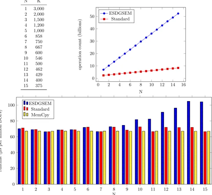
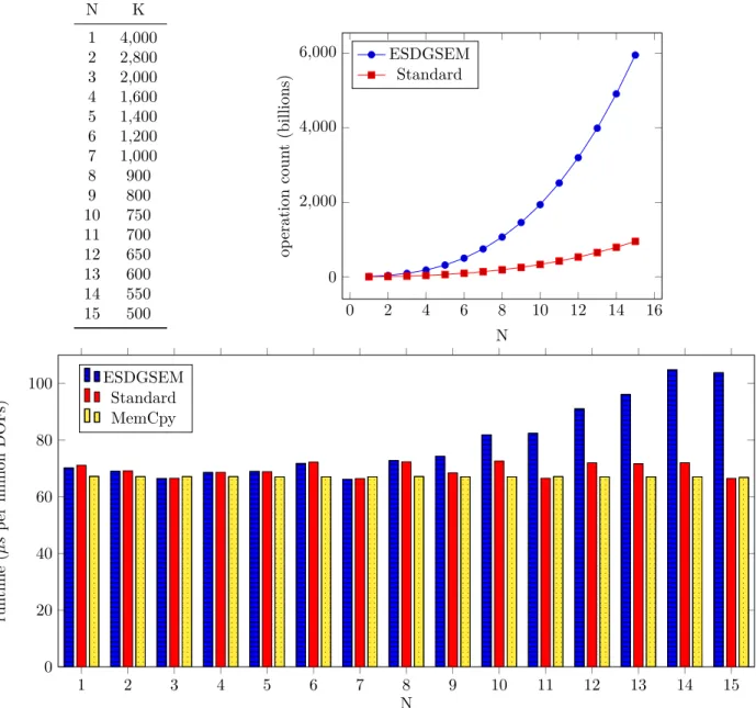
Our third, and final, contribution is to implement the two-dimensional positive ESDGSEM on GPUs.

The entropy stable approximation is built with specific split forms, which are linear combinations of the conservative and advective forms of the shallow water equations [17, 46]. However, the method remains fully conservative [11] albeit with additional computational complexity in the form of an increased number of arithmetic operations, but without the need for more data storage and transfer. Therefore, the ESDGSEM seems a perfect candidate for implementation on GPUs. We demonstrate that this expectation is true through careful analysis and detailed discussion of how to implement the numerical method into a unified approach for multi-threading languages OCCA [30].

This work is organized as follows: In Sec. 2 we briefly provide background details of the ESDGSEM described in [46] that serves as the baseline scheme. Next, shock capturing by way of artificial viscosity is discussed in Sec. 3. A positivity preserving limiter is presented in Sec. 4 that maintains the entropy stability of the DGSEM. Implementation details and analysis of the ESDGSEM compared to the standard DGSEM on GPUs is given in Sec. 5. Numerical results that exercise and test the capabilities of the positive ESDGSEM are provided in Sec. 6. Concluding remarks are given in the final section.

2. Entropy Stable Discontinuous Galerkin Spectral Element Method

We briefly present the ESDGSEM developed in [17, 46, 47] which we will extend in the following sections.

The entropy stable scheme is based on a nodal DG approximation to the split-form shallow water equations on curved quadrilateral meshes. We start with a brief description of the curvilinear transformations and numerical approximations before summarizing the main properties of the ESDGSEM in Lemma 1. We refer to [19, 24] for a more thorough derivation of DG methods and to [6, 16, 46] for a background on the entropy stable split form DG framework.

2.1. Curvilinear mappings

We separate the domain into K non-overlapping elements Ek µ and proceed by constructing a mapping on each element between the computational reference elementE= [≠1,1]²with coordinates (›,÷) and the physical coordinates (x, y). We use a transfinite interpolation with linear blending [24], where the Jacobian is computed by

J =x›y÷≠x÷y›. (2.1)

The gradients in physical spaceÒ=1

ˆ ˆx,_ˆy^ˆ 2T

and computational space ˆÒ=1

ˆ ˆ›,_ˆ÷^ˆ 2T

are related by the chain rule

Ò= 1 J

3 y÷ ≠y›

≠x÷ x›

4Òˆ. (2.2)

With a sufficiently smooth mapping we can use (2.2) to replace the physicalxand y derivatives in (1.2) to obtain the PDE in reference space

Jw˛t+ ˆÒ·(f,˛˜˛˜g)^T =S˛˜, (2.3) where we introduce the contravariant fluxes defined by

˛˜

f(w) =˛ y÷f˛(w)˛ ≠x÷˛g(˛w),

˛˜

g(w) =˛ ≠y›f˛(˛w) +x›˛g(w),˛ (2.4) and the gradient of the bottom topography transforms by (2.2) to create the contravariant source term S˛˜ given by

S˜1= 0,

S˜2=≠gh(y÷bx≠y›by), S˜³=≠gh(≠x÷bx+x›by).

(2.5)

To find the weak form of the balance law in reference space (2.3), we multiply by a smooth test function„ and integrate over the reference element. Then we use integration by parts to move the differentiation of the fluxes, ˆÒ·(f,˛˜˛g)˜ ^T, onto the test function. We replace the fluxes across element interfaces by numerical surface fluxes ˜F^ú and ˜G^ú and obtain the weak form

⁄

E

J w˛„dE +j

ˆE

„1F˛˜^ú,G˛˜^ú2

·˛ndS≠

⁄

E

1f,˛˜˛g˜2

·Òˆ„dE =⁄

E

˛˜

S„dE. (2.6)

Integrating by parts once more yields the strong form

⁄

E

J w˛„dE +j

ˆE

„1F˛˜^ú≠f,˛˜G˛˜^ú≠˛g˜2

·˛ndS +⁄

E

Òˆ ·1f,˛˜˛˜g2^T

„dE =⁄

E

˛˜

S„dE. (2.7)

2.2. Numerical Approximations

We approximate quantities of interest such as variables w˛ and fluxes f˛,˛g by polynomials of degreeN and denote them by capital lettersW˛ or F˛ and G. We use a nodal form of the interpolation with nodes˛ defined at the Legendre-Gauss-Lobatto (LGL) points{›i}^Ni=0 and{÷j}^Nj=0 in the reference square. We write the element-wise polynomial approximation (e.g. for a componentW ofW˛ ) as

w(x, y, t)--_E

k=w(x(›,÷), y(›,÷), t)¥W(›,÷, t) :=

ÿN i=0

ÿN j=0

Wi,j(t)¸i(›)¸j(÷), (2.8) where {Wi,j(t)}^N,Ni,j=0 are the time dependent nodal degrees of freedom and the one-dimensional Lagrange basis functions for the interpolant are

¸j(›) = ŸN i=0,i,j

›≠›i

›j≠›i

, j= 0, . . . , N. (2.9)

Derivatives are approximated element-wise directly from the derivative of the polynomial approximation, e.g.,

ˆ

ˆ›W(›,÷, t) = ÿN

i=0

ÿN j=0

Wi,j(t) ˆ

ˆ›¸i(›)¸j(÷). (2.10)

We introduce the polynomial derivative operatorDwith entries Dij:= ˆ¸j

ˆ›

-- -- -_›=›

i

, i, j= 0, . . . , N, (2.11)

which is used to calculate the derivative with respect to › at the interpolation nodes. It follows from the tensor product ansatz that the same derivative operatorD can be used to evaluate derivatives in› and ÷ direction. We also approximate integrals numerically using LGL quadrature and define the mass matrix M= diag(Ê0,Ê₁, . . . ,ÊN) with LGL quadrature weights on the diagonal. By the tensor product ansatz the two-dimensional quadrature is

⁄1

≠1

⁄1

≠1

w(›,÷) d›d÷¥ ÿN i=0

ÿN j=0

w(›i,÷j)ÊiÊj. (2.12)

We choose the test function„in (2.6)-(2.7) to be a polynomial in the reference element E

„^E= ÿN i=0

ÿN j=0

„^E_i,j¸i(›)¸j(÷). (2.13)

This choice of test functions and the collocation of the interpolation and quadrature nodes enables us to use the Kronecker delta property of the Lagrange interpolating polynomials to greatly simplify the integrals in (2.6). For example, the integral on the time derivative term becomes

⁄

E

JWt¸i(›)¸j(÷) dE¥J^ij(Wt)ijÊiÊj. (2.14) A significant advantage of the LGL quadrature nodes is that the corresponding derivative operatorD(2.11) and the mass matrixMsatisfy the summation-by-parts (SBP) property,

MD+ (MD)^T = diag(≠1,0, . . . ,0,1), (2.15) for all polynomial orders [14]. The SBP property enables us to make a connection between LGL-based discontinuous Galerkin methods and sub-cell finite volume type differencing methods as proposed by Fisher and Carpenter [11]. In [46] we used this relation to develop an entropy stable discontinuous Galerkin spectral element method for the shallow water equations on curvilinear geometries. The SBP property (2.15) also impliesD=≠S+ ˆDwith surface matrixS:= diag1₁

Ê₀,0, . . . ,0,≠ʹN

2andDˆ :=≠M^≠1DM. It also follows that strong and weak form discretizations are equivalent [25]. We rewrite the derivative operatorDin the computations to incorporate the surface parts and a factor of 2 for the interior that stems from the split form approach [16]

D˜ := 2D+S. (2.16)

The full discretization as well as a summary of the main properties of the ESDGSEM can be found in Lemma 1. We refer to [46] for the detailed proofs and derivations. As a notational convenience we introduce jump J·Kand average{{·}}operators which are defined by

JWK:=W⁺≠W^≠, {{W}}:= 1

2!

W⁺+W^≠"

. (2.17)

We note that jumps only occur on element interfaces and have an orientation. The “+” and “≠” states here are strictly related to the normal vector on the interface and the normal is always pointing outward from the “≠” element and into the “+” element. The averages are also used for the evaluation of the interior two point fluxes and have no orientation, but require special compact notation. For example, in the›≠direction, the interior arithmetic mean is

{{·}}(i,m),j =1 2

1(·)_ij+ (·)_mj2

. (2.18)

Lemma 1 (ESDGSEM). The semi-discrete split DG approximation to the two dimensional shallow water equations on curvilinear grids

JW˛t+L˛^›+L˛^÷=S˛˜ (2.19)

with 1

L˛^›2

ij = 1 Êi

3

”iN

ËF˛˜^ú,esÈ

N j≠”_i0ËF˛˜^ú,esÈ

0j

4+ ÿN m=0

D˜imF˛˜_(i,m),j, 1L˛^÷2

ij = 1 Êj

1”N j

ËG˛˜^ú,esÈ

iN≠”0j

ËG˛˜^ú,esÈ

i0

2+ ÿN m=0

D˜jmG˛˜_i,(m,j),

(2.20)

with curvilinear volume fluxes

˛˜

F_(i,m),j :=F˛^#(W˛i,j,W˛m,j){{y÷}}(i,m),j≠G˛^#(W˛i,j,W˛m,j){{x÷}}(i,m),j,

˛˜

G_i,(m,j):=≠F˛^#(W˛i,j,W˛i,m){{x›}}i,(j,m)+G˛^#(W˛i,j,W˛i,m){{y›}}i,(j,m),

(2.21)

where the entropy conserving two-point volume fluxes are defined by

F˛^#(W˛i,j,W˛m,j) :=

Q ca

{{hu}}(i,m),j

{{hu}}(i,m),j{{u}}(i,m),j +g {{h}}²(i,m),j≠¹2g)) h²**

(i,m),j

{{hu}}(i,m),j{{v}}(i,m),j

R db,

G˛^#(W˛i,j,W˛i,m) :=

Q ca

{{hv}}i,(m,j)

{{hv}}i,(m,j){{u}}i,(m,j)

{{hv}}i,(m,j){{v}}i,(m,j)+g {{h}}²i,(m,j)≠¹₂g)) h²**

i,(m,j)

R db.

(2.22)

The numerical interface flux in normal direction is given by

˛˜

F^ú,es=nxF˛^ú,es+nyG˛^ú,es, (2.23) and is a combination of the fluxes inxandy direction

F˛^ú,es=F˛^ú,ec≠1 2Rf

-- _f--Rf^TJ˛qK, G˛^ú,es=G˛^ú,ec≠1

2Rg-- g--R^T_g J˛qK,

(2.24)

which include the entropy conserving fluxes F˛^ú,ec and G˛^ú,ec as well as an entropy stable dissipation term which depends on the scaled flux eigenvalues

-- _f--= 1 2g

Q a

--{{u}}+{{c}}-- 0 0 0 2g--{{h}} {{u}}-- 0 0 0 --{{u}}≠{{c}}--

R b,

-- _g--= 1 2g

Q a

--{{v}}+{{c}}-- 0 0 0 2g--{{h}} {{v}}-- 0 0 0 --{{v}}≠{{c}}--

R b,

(2.25)

and eigenvectors

Rf = Q

a 1 0 1

{{u}}+{{c}} 0 {{u}}≠{{c}}

{{v}} 1 {{v}}

R b,

Rg= Q

a 1 0 1

{{u}} 1 {{u}}

{{v}}+{{c}} 0 {{v}}≠{{c}}

R b,

(2.26)

and the jump in entropy variablesJ˛qKand wave speedc= Ôgh. The entropy conserving interface fluxes are

F˛^ú,ec(W˛ ⁺,W˛ ^≠) :=

Q ca

{{h}} {{u}}

{{h}} {{u}}²+¹₂g )) h²**

{{h}} {{u}} {{v}}

R db,

G˛^ú,ec(W˛ ⁺,W˛ ^≠) :=

Q ca

{{h}} {{v}}

{{h}} {{u}} {{v}}

{{h}} {{v}}²+¹₂g )) h²**

R db,

(2.27)

and the components of the dissipation term can be found in Appendix B. The source term discretization S˛˜ is defined by

( ˜S1)ij := 0, ( ˜S2)ij := g

2!

≠hbx+Si,j^x,ú

"

, ( ˜S³)ij := g

2!

≠hby+Si,j^y,ú

"

,

(2.28)

where the additional interface penalty termsS^·,ú that account for possibly discontinuous bottom topographies can be found in [46] and the derivatives of the bottom topography are discretized in split form

(bx)ij = (y÷)ij

ÿN m=0

2Dimbmj+ ÿN m=0

2Dim(y÷b)mj≠(y›)ij

ÿN m=0

2Djmbim≠ ÿN m=0

2Djm(y›b)im,

(by)ij = (x÷)ij

ÿN m=0

2Dimbmj+ ÿN m=0

2Dim(x÷b)mj≠(x›)ij

ÿN m=0

2Djmbim≠ ÿN m=0

2Djm(x›b)im.

(2.29)

The scheme described above is called the ESDGSEM and has the following properties:

1.1 Discrete conservation of the mass and discrete conservation of the momentum if the bottom topography is constant.

1.2 Guaranteed dissipation of the total discrete energy, which is an entropy function for the shallow water equations. Hence it fulfills the discrete entropy inequality (1.7).

1.3 Discrete well-balanced property for arbitrary bottom topographies.

Proof. See [46]. ⌅

The semi-discrete ESDGSEM is only complete when equipped with a suitable time integrator. We previously used a low storage Runge-Kutta scheme in [46] but have now switched to a strong stability preserving Runge-Kutta scheme (SSPRK). This choice is necessary for the positivity preservation proof in Section 4. We use the SSPRK method that is frequently used in wet/dry shallow water schemes as in [50]

and shock capturing schemes as in [39]. The three stage scheme is W⁽¹⁾=Wⁿ+ tR(Wⁿ), W⁽²⁾= 3

4Wⁿ+1 4

1W⁽¹⁾+ tR1 W⁽¹⁾22

, Wⁿ⁺¹= 1

3Wⁿ+2 3

1W⁽²⁾+ tR1 W⁽²⁾22

,

(2.30)

whereRdenotes the spatial ESDGSEM operator R=≠1 J

1L˛^›+L˛^÷≠S˛˜2

. (2.31)

3. Artificial Viscosity

The entropy stable scheme is more robust compared to a standard DGSEM for the shallow water equations [17, 46], but it is not oscillation free in the presence of shocks. These oscillations might lead to unphysical solutions and cause simulations to crash if the water height becomes negative. We discuss the addition of a positivity limiter in the next section. Usually, such positivity preserving limiters are coupled with some form of TVB limiter [52] or artificial viscosity [28] to keep oscillations in check. Our main requirement for the additional smoothing or limiting is to preserve the entropy stability of the scheme. In [15] the authors prove that under certain conditions, adding artificial viscosity to the scheme maintains the entropy stability.

We choose the gradient variables carefully and use the discretization by Bassi and Rebay [1] to fulfill these conditions analogous to the strategy in [15]. For our shock capturing, we only add artificial viscosity to the momentum equations. While the smoothing is weaker without direct artificial viscosity in the continuity equation, we trivially maintain conservation of mass and have a straight forward mapping to the entropy variables, which leads to an easy proof of the requirements for the entropy stability via a theorem from [15]. In fact, we choose the entropy variables q1=uand q2=v as gradient variables, leading to a simple one-to-one mapping from gradient variables to entropy variables. We scale the gradient by the water height

hand a viscosity parameter‘to obtain the viscous fluxes. The viscosity parameter is dynamically computed for each element and is based on a smoothness measure of the water height within the element. We give details on the computation of the viscosity parameter in Appendix A. The modified shallow water equations with artificial viscosity are

ht+ (hu)x+ (hv)y = 0,

(hu)t+ (h u²+g h²/2)x+ (huv)y =≠g h bx+Ò·1 h‘ ˛U2

, (hv)t+ (huv)x+ (h v²+g h²/2)y =≠g h by+Ò·1

h‘ ˛V2 , U˛ =Òu,

V˛ =Òv,

(3.1)

or in compact flux form

˛

wt+Ò·(f,˛˛g)^T =S˛+Ò·(f˛^v,˛g^v)^T, U˛ =Òu,

V˛ =Òv,

(3.2)

with viscous fluxes f˛^v(w,˛ U˛,V˛) = h‘(0,U¹,V¹)^T and ˛g^v(˛w,U˛,˛V) = h‘(0,U²,V²)^T. We include the new viscous fluxes into the flux divergence and get

Jw˛t=≠Òˆ ·(f˛˜+f˛˜^v,˛g˜+˛g˜^v)^T +S˛˜, JU˛ =3

y÷ ≠y›

≠x÷ x›

4Òˆu,

J˛V=3

y÷ ≠y›

≠x÷ x›

4Òˆv,

(3.3)

where we transform the physical gradient operator with the metrics of the element mappings.

Analogous steps as in Sec. 2 are then used to find the weak and strong form and their discretizations for the continuity and momentum equations. We multiply the transformed gradient equations by the same test function„and integrate over the domain to find the weak form

⁄

E

J U˛„dE≠ j

ˆE

„U^ú˛ndS +⁄

E

u

3 y÷ ≠y›

≠x÷ x›

4Òˆ„dE = 0,

⁄

E

J ˛V„dE≠ j

ˆE

„V^ú˛ndS +⁄

E

v

3 y÷ ≠y›

≠x÷ x›

4Òˆ„dE = 0,

(3.4)

where U^ú and V^ú are the numerical interface states for the gradient equations. We discretize the weak form gradient equations (3.4) and use the Lagrange property to simplify. For example, the volume integral approximations for theU˛ equations are

⁄1

≠1

⁄1

≠1

u 3

y÷

ˆ

ˆ›(¸i(›)¸j(÷))≠y›

ˆ

ˆ÷(¸i(›)¸j(÷))4

d›d÷¥ ≠ ÿN m=0

Dˆimumjy÷mjÊiÊj+ ÿN n=0

Dˆjnuiny›inÊiÊj,

⁄1

≠1

⁄1

≠1

u 3

≠x÷

ˆ

ˆ›(¸i(›)¸j(÷)) +x›

ˆ

ˆ÷(¸i(›)¸j(÷))4

d›d÷¥ ÿN m=0

Dˆimumjx÷mjÊiÊj≠ ÿN n=0

Dˆjnuinx›inÊiÊj. (3.5)

Similarly, the surface integrals forU˛ are approximated by j

ˆE

„U^ú˛n₁dS¥ ≠”_i0U_i0^úy÷i0Êj+”iNU_iN^ú y÷i0Êj≠”_j0U_0j^úy›0jÊi+”jNU_{N j}^ú y›N jÊi, j

ˆE

„U^ú˛n2dS¥ ≠”i0U_i0^úx÷i0Êj+”iNU_iN^ú x÷i0Êj≠”j0U_0j^úx›0jÊi+”jNU_{N j}^ú x›N jÊi.

(3.6)

We summarize the ESDGSEM with artificial viscosity and state the full discretizations of all the new viscous terms and gradient equations in Theorem 1 and proof that the resulting method is entropy stable.

Theorem 1(Entropy stability of ESDGSEM with artificial viscosity).The ESDGSEM (2.19)with additional viscous terms as in (3.1)is

JW˛t+L˛^›+L˛^÷=S˛˜+L˛^v›+L˛^v÷. (3.7) The viscous termsL˛^v›,L˛^v÷ are discretized in strong form by

(L˛^v›)ij = ÿN m=0

Dim(F˛˜^v)mj+ 1 Êi

1”iNF˛˜_{N j}^v,ú≠”i0F˛˜_0j^v,ú2

≠ 1 Êi

1”iNF˛˜_{N j}^v ≠”i0F˛˜_0j^v2 , (L˛^v÷)ij =

ÿN m=0

Djm(G˛˜^v)im+ 1 Êj

1”N jG˛˜^v,_iN^ú≠”0jG˛˜^v,_i0^ú2

≠ 1 Êj

1”N jG˛˜^v_iN≠”0jG˛˜^v_i02 .

(3.8)

The curvilinear viscous fluxes are defined with the BR1 approach as

˛˜

F^v= y÷F˛^v≠x÷G˛^v,

˛˜

G^v= ≠y›F˛^v+x›G˛^v,

(3.9) with viscous fluxes

F˛^v=h‘(U1,V1)^T,

G˛^v=h‘(U2,V2)^T, (3.10)

and the viscous flux interface coupling is computed with

˛˜

F^v,ú=ÓÓF˛˜^vÔÔ ,

˛˜

G^v,ú=ÓÓG˛˜^vÔÔ .

(3.11)

The gradients U˛ =Òuand˛V=Òv are computed by (U1)ij= (y÷)ij

ÿN m=0

Dˆimumj≠(y›)ij

ÿN m=0

Dˆjmuim+(y÷)ij

Êi

!”iNU_{N j}^ú ≠”_i0U_0j^ú"+(y›)ij

Êj (”N jU_iN^ú ≠”_0jU_i0^ú) (U2)ij=≠(x÷)ij

ÿN m=0

Dˆimumj+ (x›)ij

ÿN m=0

Dˆjmuim+(x÷)ij

Êi

!”iNU_{N j}^ú ≠”_i0U_0j^ú"+(x›)ij

Êj (”N jU_iN^ú ≠”_0jU_i0^ú) (V1)ij= (y÷)ij

ÿN m=0

Dˆimvmj≠(y›)ij

ÿN m=0

Dˆjmvim+(y÷)ij

Êi

!”iNV_{N j}^ú ≠”i0V_0j^ú"+(y›)ij

Êj

(”N jV_iN^ú ≠”0jV_i0^ú)

(V²)ij=≠(x÷)ij

ÿN m=0

Dˆimvmj+ (x›)ij

ÿN m=0

Dˆjmvim+(x÷)ij

Êi

!”iNV_{N j}^ú ≠”i0V_0j^ú"+(x›)ij

Êj

(”N jV_iN^ú ≠”0jV_i0^ú), (3.12) where the numerical statesU^ú andV^ú are chosen according to BR1 as the average values

U^ú={{u}},

V^ú={{v}}. (3.13)

The ESDGSEM with artificial viscosity (3.7)and viscous terms discretized as in(3.8)and(3.12), is entropy stable.

Proof. In [15] the authors show that viscous terms discretized by Bassi and Rebay [1] are entropy stable if the viscous fluxes can be rewritten as the product of a symmetric, positive definite block matrixB^‘and the gradient of the entropy variables

f¡^v(˛w, Òw) =˛ B^‘Ò˛q, (3.14)

with state vectorsf^¡v =3 f˛^v

˛g^v 4

œR⁶andÒ˛q=3

˛ qx

˛ qy

4

œR⁶ . In the case of the shallow water equations, the block matrixB^‘ can be expressed as

B^‘=3 B11 B12

B21 B22

4

œR^6◊6. (3.15)

The entropy stability requirements for the block matrixB^‘ are then that each blockBij is symmetric B^‘ij=!B^‘ji

"T

, (3.16)

and positive (semi-)definite

ÿd i=1

ÿd j=1

ˆ˛q ˆxi

TB^‘_ij ˆ˛q

ˆxj Ø0, ’˛q. (3.17)

The choice of gradient variables and fluxes in (3.1) make the block matrix very simple in this case

B^‘=‘h Q cc cc cc a

0 0 0 0 0 0 0 1 0 0 0 0 0 0 1 0 0 0 0 0 0 0 0 0 0 0 0 0 1 0 0 0 0 0 0 1

R dd dd dd b

. (3.18)

We check the requirement (3.17) to find ÿ2

i=1

ÿ2 j=1

ˆ˛q ˆxi T

B^‘ij

ˆ˛q

ˆxj = (˛qx)^TB^‘₁₁˛qx+ (˛qy)^TB^‘₂₂˛qy

=‘h!

u²_x+v_x²+u²_y+v_y²"

Ø0.

(3.19)

⌅ The artificial viscosity reduces the amount and magnitude of oscillations as shown in the numerical results section, specifically in a dam break example in Section 6.5.

4. Positivity Preserving Limiter

The artificial viscosity from Sec. 3 greatly reduces the oscillations, but in cases with wet/dry regions, this is sometimes not enough as even small oscillations may render a numerical scheme unstable if they lead to negative water heights. A mechanism is needed, that strictly enforces the positivity of the water height h without destroying accuracy, conservation, well-balancedness or entropy-stability of the ESDGSEM. In, e.g., [35, 49, 50, 52] the authors have developed a positivity preserving limiter and applied it to the shallow water equation. The limiter is based on a linear scaling around element averages and thus relies on non- negative average water heights in all elements. It is then proved that non-negative average water heights are guaranteed to be preserved for an Euler time step. The proof relies on the specific choice of the numerical

flux. Numerical fluxes that preserve non-negative water heights for finite volume schemes are called positivity preserving [52]. For Cartesian meshes, this property directly translates to DG methods by way of selecting any positivity preserving numerical interface fluxes, e.g. [50]. In [52] it is proven that the Lax-Friedrichs numerical flux [35] is positivity preserving and the same is noted for the Godunov flux [10], Boltzmann type flux [34] and the Harten-Lax-van-Leer flux [18]. The positivity preserving property is shown for Euler time integration but naturally extends to SSPRK methods, e.g. (2.30), as these are convex combinations of Euler time steps, see [38] for details.

In this section we prove that the entropy stable numerical flux of the ESDGSEM (2.23) is positivity preserving in the sense that non-negative mean water heights are preserved for one Euler time step. On Cartesian meshes it is possible to prove this similarly to [52], where the update of the mean water height is written in finite volume form. Due to generally different Jacobians of the curvilinear mappings and possible changing normals on opposing sides this is not as straightforward on curved meshes. We directly prove the positivity preservation for curved quadrilateral meshes in Lemma 2. Also, we verify that the positivity preserving limiter is entropy stable in Lemma 3. Both results are then summarized in Theorem 2.

We will now show that the ESDGSEM with Euler time integration preserves a non-negative water height for a sufficiently small time step. For notational convenience we use the notation Wj,s (opposed toWij for internal nodal values) to denote the value of W at node j on interface s, wheresœ{1, . . . ,4} denotes the element local interface number. We also introduce the surface Jacobian J^surf on › = ±1 (s = 2,4) and

÷=±1 (s= 1,3) interfaces by

J^surf:= 

y›y›+x›x›, for÷=±1, J^surf:= 

y÷y÷+x÷x÷, for›=±1. (4.1) Lemma 2 (Preservation of non-negative mean water heights in ESDGSEM). If the water height, h, is non-negative for all LGL nodes then the average water height in the next time step is non-negative for all elements under the additional time step restrictions

tÆ Ê₀aj,s

1Aj,s+ 2{{u˜}}j,s

2,

tÆ -- -- -

Ê0aj,sg hj,s

{{c}}j,sBj,sJ˜uKj,s

-- --

-, only ifhj,s>0,

(4.2)

where we introduce the rotated normal velocity

˜

u:=nxu+nyv (4.3)

for all edge nodes j= 0, . . . , N on all element sides s= 1, . . . ,4, and A:=--{{u˜}}+{{c}}--+--{{u˜}}≠{{c}}--,

B:=--{{u˜}}+{{c}}--≠--{{u˜}}≠{{c}}--. (4.4) For the Legendre Gauss Lobatto nodes, the quadrature weight Ê0 is given byÊ0=¹₂N(N≠1). We also have geometric scaling factors on the interfaces given by aj,s:= ^Jj,s

Jj,s^surf

with volume and surface Jacobians defined in (2.1)and (4.1).

Proof. We first examine the numerical flux. Since the shallow water equations are rotationally invariant, we can calculate the numerical flux in normal direction and then rotate back. We want to guarantee positive water height and, thus, proceed to examine the numerical flux contributions for the water height equation.

The first entry of the entropy stable numerical flux in the normal direction can be simplified to F₁^ú,es(W˛˜⁺,W˛˜^≠) ={{h}} {{u˜}}≠ 1

4g(AJgh+gbK+{{c}}BJu˜K), (4.5)

where ˜u=nxu+nyv and full details on the derivation of (4.5) are given in Appendix B. As the ESDGSEM is a conservative numerical scheme, we can write the update of the element average water height in one Euler time step as

h^tn+1=h^tn≠ t --E--

ÿ4 s=1

ÿN j=0

ÊjJj,s^surfF˜₁^ú,es!

W_j,s^int, W_j,s^ext, nj,s"

=h^tn≠ t --E--

ÿ4 s=1

ÿN j=0

ÊjJj,s^surfF₁^ú,es!W˜_j,s^int,W˜_j,s^ext"

,

(4.6)

whereJj,s^surf is the surface Jacobian at nodej on interfacesdefined in (4.1). We can also write the average water heighth^tn as

h^tn= 1 --E--

ÿN j=0

ÿN i=0

hijJ^ijÊiÊj

= 1 --E--

Nÿ≠1 i=1

Nÿ≠1 j=1

hijJ^ijÊiÊj+1 2 -1 -E--

ÿ4 s=1

Nÿ≠1 j=1

hj,sJ^j,sÊ0Êj+1 2 -1 -E--

ÿ4 s=1

ÿN j=0

hj,sJ^j,sÊ0Êj

= 1 --E--

Nÿ≠1 i=1

Nÿ≠1 j=1

hijJ^ijÊiÊj+1 2 1

--E-- ÿ4 s=1

Nÿ≠1 j=1

hj,sJ^j,sÊ₀Êj

+ 1 2--E--

ÿN j=0

hj,3Jj,3Ê0Êj+ 1 2--E--

ÿN j=0

hj,1Jj,1Ê0Êj

+ 1 2--E--

ÿN i=0

h_j,4Jj,4Ê₀Êj+ 1 2--E--

ÿN i=0

h_j,2Jj,2Ê₀Êj.

(4.7)

Inserting the new expression for the average water height (4.7) into the update scheme (4.6) we find

h^tn+1 = 1 --E--

Nÿ≠1 i=1

Nÿ≠1 j=1

hijJ^ijÊiÊj+1 2 1

--E-- ÿ4 s=1

Nÿ≠1 j=1

hj,sJ^j,sÊ₀Êj

+ 1 --E--

ÿN j=0

Jj,1Ê0Êj

51

2hj,1≠ t

Ê0aj,1F₁^ú,es!W˜_j,1^int,W˜_j,1^ext"6 + 1

--E-- ÿN

j=0Jj,3Ê₀Êj

51

2h_j,3≠ t

Ê₀a_j,3F₁^ú,es!W˜_j,3^int,W˜_j,3^ext"6 + 1

--E-- ÿN

j=0Jj,2Ê0Êj

51

2hj,2≠ t

Ê0aj,2F₁^ú,es!W˜_j,2^int,W˜_j,2^ext"6 + 1

--E-- ÿN

j=0Jj,4Ê₀Êj

51

2h_j,4≠ t

Ê₀a_j,4F₁^ú,es!W˜_j,4^int,W˜_j,4^ext"6 ,

(4.8)

with aj,s := _J^Jsurf^j,s

j,s . We note that for the special case of uniform Cartesian meshes this factor is simply aj,s = y for s= 1,3 and aj,s = xfor s= 2,4. The first two sums are clearly non-negative for meshes with positive Jacobians. We proceed to examine the interface terms

1

2hj,s≠ t

Ê0aj,sF₁^ú,es!W˜_j,s^int,W˜_j,s^ext"

, s= 1, . . . ,4 . (4.9)

We can do this for an arbitrary nodej, sides, and only need to distinguish between internal valuesW^≠ and external values W⁺ on the interface. We thus omit the indicesj and sin the following steps. By inserting

the compact expression for F₁^ú,es from (4.5) and assuming continuous bottom topographies across element interfaces we find

1

2h^≠≠ 1 4g t

Ê0a(4g{{h}} {{u˜}}≠gAJhK≠{{c}}BJu˜K)

= 1

2h^≠≠ 1 4g

t Ê0a

!gh⁺(2{{u˜}}≠A) +gh^≠(2{{u˜}}+A)≠{{c}}BJu˜K"

= 1 4

t

Ê0ah⁺(A≠2{{u˜}}) +1 4h^≠

31≠ t

Ê0a(A+ 2{{u˜}})4 +1

4 3

h^≠+ t

gÊ0a{{c}}BJu˜K 4

(4.10)

We examine the three terms in (4.10) individually. The first term is always non-negative, since

A=--{{u˜}}+{{c}}--+--{{u˜}}≠{{c}}--Ø2--{{u˜}}--. (4.11) For the second term we require an additional time step condition. From

31≠ t

Ê₀a(A+ 2{{u˜}})4 _!

Ø0, (4.12)

we find

tÆ^! Ê₀a

(A+ 2{{u˜}}). (4.13)

For the third term, we cannot generally factor outh^≠, so we need to treat this carefully. We need to show that the last term is not negative in the cases h^≠ = 0 andh⁺ = 0 as well as in the wet case where both water heights are positive. In the case h^≠ = 0, we also have ˜u^≠ = 0 and thus we see Ju˜K = ˜u⁺, and the whole term becomes

t

gÊ₀a{{c}}Bu˜⁺. (4.14)

We note that{{c}}is always non-negative, so we must examine the signs of B and ˜u⁺. The velocity can have an arbitrary sign but from the definition ofB

B=--{{u˜}}+{{c}}--≠--{{u˜}}≠{{c}}--=----1

2u˜⁺+{{c}}

-- --≠

-- --1

2u˜⁺≠{{c}}

--

--, (4.15) we see that the sign ofB matches the sign of ˜u⁺ and thus the whole term is guaranteed non-negative for h^≠ = 0 and h⁺ Ø0. If h^≠ >0 (and thus in general ˜u^≠ ,0), we are allowed to factor out h^≠. Then we require

t gÊ0a

{{c}}BJ˜uK h^≠

Ø ≠! 1. (4.16)

This condition guarantees non negativity for the third term in (4.10) and can only be violated ifBJu˜K<0.

There are two sets of conditions where this is the case. Either we have ˜u^≠ > u˜⁺ and {{u˜}} > 0, which implies ˜u^≠>0. Or, alternatively, we have B <0 andJu˜K>0, which implies 0>u˜⁺ >u˜^≠. In either way, forBJ˜uK<0, we can guarantee non negativity by enforcing the additional time step restriction

tÆ^! -- -- -

gÊ₀a h^≠ {{c}}BJu˜K

-- --

-. (4.17)

This proof for one Euler time step extends to SSPRK methods as used in the ESDGSEM as seen in, e.g.,

[50]. ⌅

While Lemma 2 guarantees a non-negative average water height in the next time step, we still need to ensure point-wise non-negativity. We use the limiter applied to the shallow water equations by Xing et al [50] and developed in [35, 49, 52] which is a linear scaling around the element average

„˛ Wij =◊1

W˛ij≠W˛ E

2+W˛ E, (4.18)