Technical Report Series
Center for Data and Simulation Science
Alexander Heinlein, Christian Hochmuth, Axel Klawonn
Monolithic Overlapping Schwarz Domain Decomposition Methods with GDSW Coarse Spaces for Saddle Point Problems
Technical Report ID: CDS-2018-1
Available at http://kups.ub.uni-koeln.de/id/eprint/8355
Submitted on July 02, 2018
DECOMPOSITION METHODS WITH GDSW COARSE SPACES FOR SADDLE POINT PROBLEMS
ALEXANDER HEINLEIN
† ‡, CHRISTIAN HOCHMUTH
†, AND AXEL KLAWONN
† ‡Abstract. Monolithic overlapping Schwarz preconditioners for saddle point problems of Stokes, Navier-Stokes, and mixed linear elasticity type are presented. For the first time, coarse spaces ob- tained from the GDSW (Generalized Dryja–Smith–Widlund) approach are used in such a setting.
Numerical results of our parallel implementation are presented for several model problems. In partic- ular, cases are considered where the problem cannot or should not be reduced using local static con- densation, e.g., Stokes, Navier-Stokes or mixed elasticity problems with continuous pressure spaces.
In the new monolithic preconditioners, the local overlapping problems and the coarse problem are saddle point problems with the same structure as the original problem. Our parallel implementation of these preconditioners is based on the FROSch (Fast and Robust Overlapping Schwarz) library, which is part of the Trilinos package ShyLU. The implementation is algebraic in the sense that the preconditioners can be constructed from the fully assembled stiffness matrix and information about the block structure of the problem. Parallel scalability results for several thousand cores for Stokes, Navier-Stokes, and mixed linear elasticity model problems are reported. Each of the local problems is solved using a direct solver in serial mode, whereas the coarse problem is solved using a direct solver in serial or MPI-parallel mode or using an MPI-parallel iterative Krylov solver.
Key words. Saddle point problems, Stokes, Navier-Stokes, almost incompressible linear elastic- ity, GDSW, monolithic overlapping Schwarz, algebraic preconditioner, parallel computing, domain decomposition
AMS subject classifications. 65F10, 65M55, 65Y05, 65F08
1. Introduction. Saddle point problems arise in many physical applications, e.g., in the simulation of fluid flow or almost incompressible materials. We consider finite element discretizations of the underlying partial differential equations which can result in large and ill-conditioned linear systems. In addition to the required inf-sup conditions for finite element discretizations of saddle point problems, special care has to be taken when constructing preconditioners for the discrete problem. In particular, the block structure and the coupling blocks have to be handled appropriately to guarantee fast convergence of iterative methods.
In this paper, we propose a monolithic two-level overlapping Schwarz precondi- tioner with discrete harmonic coarse space. Specifically, we extend GDSW (General- ized Dryja–Smith–Widlund) coarse spaces, which were originally introduced for scalar elliptic problems in [18, 19], to general saddle point problems. For elliptic problems, the GDSW coarse basis functions are energy minimal extensions representing the null space of the elliptic operator. In the previous works [20, 21] by Dohrmann and Wid- lund on GDSW preconditioners for saddle point problems, only discontinuous pressure spaces were considered. Consequently, the saddle point problems could be reduced to elliptic problems by static condensation of the pressure. In contrast, our method is inspired by the monolithic Schwarz preconditioners with Lagrangian coarse basis functions introduced by Klawonn and Pavarino in [48, 49], which operates on the full saddle point problem. The coarse basis functions of our new monolithic GDSW
†
Department of Mathematics and Computer Science, University of Cologne, Weyertal 86- 90, 50931 K¨ oln, Germany, alexander.heinlein@uni-koeln.de, christian.hochmuth@uni-koeln.de, axel.klawonn@uni-koeln.de, url: http://www.numerik.uni-koeln.de
‡
Center for Data and Simulation Science, University of Cologne, Germany, url: http://www.cds.
uni-koeln.de
1
preconditioner are discrete saddle point harmonic extensions of interface functions.
One significant advantage of our new method is that it can be applied to arbitrary geometries and domain decompositions, whereas the use of Lagrangian coarse basis functions requires a coarse triangulation. This limits the use of Schwarz methods with Lagrangian coarse spaces for arbitrary geometries.
In [21, 22, 23], different approaches for reducing the dimension of GDSW coarse spaces have been introduced and some of them have been proven to significantly im- prove the parallel scalability compared to standard GDSW coarse spaces; cf. [40].
Alternatively, the parallel scalablity could be improved by solving the coarse level in- exactly using another GDSW preconditioner resulting in a three-level GDSW method;
cf. [39]. For highly heterogeneous multiscale problems, GDSW coarse spaces were en- hanced using local generalized eigenvalue problems in [34, 33], resulting in a method that is robust with respect to the contrast of the coefficients.
As described in [36], in a parallel implementation, GDSW coarse spaces can be constructed in an algebraic fashion directly from the fully assembled matrix. The parallel implementation of our new Schwarz preconditioners with GDSW coarse spaces for saddle point problems is based on the FROSch software [35] in the package ShyLU of the Trilinos library [41]. FROSch is a framework for Schwarz preconditioners in Trilinos and one of its main contributions is a parallel and algebraic implementation of the GDSW preconditioner for elliptic problems; see also [31, 38, 37, 36, 40]. Therefore, the parallel implementation described here is also algebraic, i.e., the preconditioner can be easily built requiring only few input parameters, and will be described in more detail in section 7. The functionality of our new implementation will be added to FROSch in the near future and will therefore be available as open source as part of Trilinos.
In our approach, we solve saddle point problems of the form (1) using the GM- RES Krylov subspace method. We consider the Stokes and Navier-Stokes equa- tions as well as a mixed formulation for linear elasticity in two and three dimen- sions. An extensive overview of numerical methods for saddle point problems is given in [6]. Older approaches for the iterative solution of those saddle point prob- lems are, e.g., the exact and inexact Uzawa algorithm [1, 3, 12, 27, 55, 69], where velocity and pressure are decoupled and solved in a segregated approach. Other physically based approaches are the SIMPLE (Semi-Implicit Method for Pressure Linked Equations) method and its generalizations, i.e., SIMPLEC and SIMPLER;
cf. [25, 51, 52]. Block preconditioners for the (generalized) minimum residual method and conjugate residual method are presented in [26, 56, 60, 62, 66, 46, 49, 47, 50].
Further block preconditioners are the PCD (Pressure Convection-Diffusion) precondi- tioner [61, 45, 29], the LSC (Least-Squares Commutator) preconditioner [24], Yosida’s method [53, 54], the Relaxed Dimensional Factorization (RDF) preconditioner [8] and the Dimensional Splitting (DS) preconditioner [7, 17]. Domain decomposition meth- ods for Stokes and Navier-Stokes problems were studied in [11, 69]. Schwarz pre- conditioners for saddle point problems have already been used for the approximation of the inverse matrices of blocks in [15, 2, 16, 36] and as monolithic preconditioners in [63, 14, 4, 5, 68]. Alternative solvers for saddle point problems are, e.g., multigrid methods; cf. [65, 64, 67, 10, 13, 43, 30]. Let us note that there are several other publications on iterative solvers for saddle point problems.
The paper is arranged as follows. In section 2, we present the model problems. In
section 3, we describe the mixed finite elements used in our discretization. Then, we
recapitulate the definition of two-level Schwarz preconditioners for elliptic problems
in section 4 and explain energy-minimizing GDSW coarse spaces. In section 5, we de-
scribe monolithic two-level Schwarz preconditioners for saddle point problems. First, we introduce a monolithic Schwarz preconditioner with Lagrangian coarse space and the new monolithic GDSW preconditioner. Furthermore, we discuss how we account for a nonunique pressure in the preconditioner in section 6. Details on the parallel and algebraic implementation of the monolithic preconditioner based on the FROSch framework is given in section 7. In section 8, we present numerical results for the three model problems.
2. Saddle point problems. We construct our monolithic preconditioner for the three model problems presented in this section. In the following we assume that Ω ⊂ R d , d = 2, 3 is a polygonal or polyhedral open set.
2.1. Stokes equations. Our first model problem is given by the Stokes equa- tions in two and three dimensions. We seek to determine the velocity u ∈ V g with V g = {v ∈ (H 1 (Ω)) d : v |∂Ω
D= g} and the pressure p ∈ L 2 0 (Ω) of an incompress- ible fluid with negligible advective forces by solving the variational formulation: find (u, p), such that
µ Z
Ω
∇u : ∇v dx − Z
Ω
div v p dx = Z
Ω
f v dx ∀v ∈ (H 0 1 (Ω)) d ,
− Z
Ω
div u q dx = 0 ∀q ∈ L 2 (Ω),
with dynamic viscosity µ and ∂Ω D = ∂Ω.
In our numerical tests, we consider the (leaky) lid-driven cavity Stokes problem;
cf. [28, Sec. 3.1], which we will denote as LDC Stokes problem : let Ω be the unit square or cube in two or three dimensions, respectively. We prescribe the velocity boundary conditions by
d = 2 : g = (1, 0) T if x 2 = 1, g = (0, 0) T if x 2 < 1, d = 3 : g = (1, 0, 0) T if x 3 = 1, g = (0, 0, 0) T if x 3 < 1.
and choose µ = 1 and f ≡ 0.
2.2. Mixed linear elasticity. Second, we consider mixed linear elasticity prob- lems describing the displacement u ∈ V and the pressure p = −λ div u ∈ L 2 0 (Ω) of a body consisting of an almost incompressible material with Lam´ e constants λ and µ.
We fix the body along Γ 0 ⊂ ∂Ω and subject material to the external body force f : find (u, p), such that
2µ Z
Ω
ε(u) : ε(v) dx − Z
Ω
div v p dx = Z
Ω
f v dx ∀v ∈ V,
− Z
Ω
div u q dx − 1 λ
Z
Ω
p q dx = 0 ∀q ∈ L 2 (Ω),
with V = {v ∈ H 1 (Ω) d : v |Γ
0= 0}. The components of the linearized strain tensor ε(u) are ε(u) ij = 1 2 (∂u i /∂x j + ∂u j /∂x i ).
While a pure displacement formulation for the linear elasticity problem suffers
from volume locking in the incompressible limit, the above mixed formulation is a
good remedy; cf. [9, Sec. 6.3]. We consider a three-dimensional model problem: let
Ω be the unit cube, f = (0.1, 0, 0) T , and Γ 0 = ∂Ω. The incompressibility of the
material is modeled by λ approaching infinity or by the Poisson ratio ν = λ/2(λ + µ)
approaching 0.5. In particular, we fix µ = 1.0 and increase λ accordingly for our
numerical tests. Further, we chose a uniformly distributed random right hand side.
Fig. 1 . Velocity of the Navier-Stokes benchmark problem; Re = 20.
2.3. Navier-Stokes equations. Third, we consider the steady-state Navier- Stokes equations modeling the flow of an incompressible Newtonian fluid with kine- matic viscosity ν > 0. We seek to determine the velocity u ∈ V g and the pressure p ∈ Q ⊂ L 2 (Ω) by solving the variational formulation: find (u, p), such that
ν Z
Ω
∇u : ∇v dx + Z
Ω
(u · ∇u) · v dx − Z
Ω
div v p dx = Z
Ω
f v dx ∀v ∈ V 0 ,
− Z
Ω
div u q dx = 0 ∀q ∈ Q,
with V 0 ⊂ (H 1 (Ω)) d . The presence of the convection term u · ∇u leads to a nonlinear system that is solved by Newton’s method or Picard iterations; cf. [28, Sec. 8.3].
We will consider two different Navier-Stokes model problems for the numerical experiments. In both cases, the source function is f ≡ 0.
The first model problem is a regularized lid-driven cavity Navier-Stokes problem, similar to the two-dimensional problem in [28, Sec. 3.1], with ∂Ω D = ∂Ω and Q = L 2 0 (Ω). We refer to as LDC Navier-Stokes problem. The boundary values of the problem are given by
d = 2 : g = (4x 1 (1 − x 1 ), 0) T if x 2 = 1, g = (0, 0) T if x 2 < 1,
d = 3 : g = (16x 1 (1 − x 1 )x 2 (1 − x 2 ), 0, 0) T if x 3 = 1, g = (0, 0, 0) T if x 3 < 1.
The second model problem is the three-dimensional Navier-Stokes benchmark for the flow around a cylinder with circular cross-section, to which we will refer as the Navier-Stokes benchmark; cf. [59], where a detailed description of the simulation setup is given. See Figure 1 for the benchmark geometry and the velocity of the solution of the Navier-Stokes benchmark. The length of the domain is 2.5m, A = 0.41m is the height and width of the domain. Further, ν = 10 −3 m/s, and we define V g = {v ∈ H 1 (Ω) d : v |∂Ω
D= g} , V 0 = {v ∈ H 1 (Ω) d : v |∂Ω
D= 0}, and Q = L 2 (Ω).
The inflow and outflow boundary conditions are u = (16u max x 2 x 3 (A − x 2 )(A − x 3 )/A 4 , 0, 0)
on ∂Ω D
in= {(0, x 2 , x 3 ) ∈ R 3 : 0 < x 2 , x 3 < A} and ν ∂u
∂n − pn = 0 on ∂Ω N = {(2.5, x 2 , x 3 ) ∈ R 3 : 0 < x 2 , x 3 < A},
respectively, with the outward pointing normal vector n and Neumann boundary ∂Ω N .
Then, the maximum velocity across the inflow is u max = 0.45m/s. On the remainder
of the boundary, we set no-slip boundary conditions.
In a dimensionless reformulation of the Navier-Stokes equations, the Reynolds number Re specifies the relative contributions of convection and diffusion. For the LDC Navier-Stokes problem in two and three dimensions, we obtain Re = 1/ν. The Reynolds number of the benchmark problem is Re = 20.
3. Finite element discretization. In general, we will use the terminology of the Stokes and Navier-Stokes equations, and therefore, we refer to u as velocity and to p as pressure. For the discretization of the saddle point problems considered here we use mixed finite elements. Therefore, we first introduce a triangulation τ h of Ω with characteristic mesh size h, which can be non-uniform. Then, we introduce the conforming discrete piecewise quadratic velocity and piecewise linear pressure spaces
V h (Ω) = {v h ∈ (C 2 (Ω)) d ∩ V : v h | T ∈ P 2 ∀ T ∈ τ h } and Q h (Ω) = {q h ∈ C(Ω) ∩ Q : q h | T ∈ P 1 ∀ T ∈ τ h },
respectively, of P2-P1 Taylor-Hood mixed finite elements.
A discrete saddle point problem has the form Ax =
A B T B −t 2 C
u h
p h
= F h
0
= b.
(1)
Note that, in contrast to mixed finite element discretizations with discontinuous pres- sure, the pressure cannot be eliminated by static condensation on the element level for continuous pressure.
For simplicity, we will drop the index h of the discrete variables for the remainder of this paper.
For the model problems considered here, the matrix B T arises from the discretiza- tion of the divergence term
Z
Ω
div v p dx .
Therefore, the null space of B T consists of all constant pressure functions. If t 6= 0 and the matrix C is symmetric positive definite, the pressure is uniquely determined.
Otherwise, the pressure has to be normalized, e.g., by restricting the pressure to the space
Q h = Q h ∩ L 2 0 (Ω),
i.e., to zero mean value. In order to do so, we can introduce a Lagrange multiplier λ to enforce
(2)
Z
Ω
p dx = 0.
This results in the block system
(3) Ax =
A B T 0 B 0 a T
0 a 0
u p λ
=
F
0 0
,
where the vector a arises in the finite element discretization of the integral (2). Al- ternatively, we can use the projection
P = I p − a T (aa T ) −1 a,
(4)
1.000e+00 8.000e+00
2 3 4 5 6 7
subdomains
1.000e+00 8.000e+00
2 3 4 5 6 7
subdomains
0.000e+00 8.000e+00
1 2 3 4 5 6 7
subdomain1
1.000e+00 8.000e+00
2 3 4 5 6 7
subdomains
0.000e+00 8.000e+00
1 2 3 4 5 6 7
subdomain1
1.000e+00 8.000e+00
2 3 4 5 6 7
subdomains
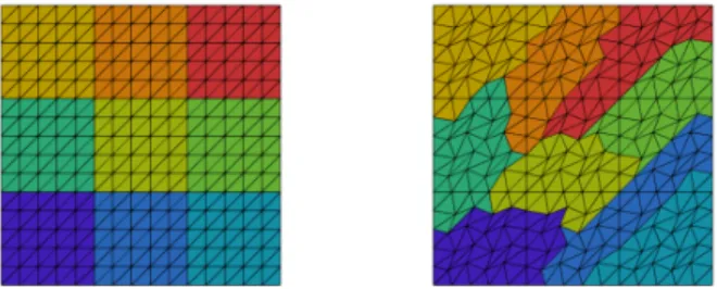
Fig. 2. Structured mesh and domain decomposition (first, second) and unstructured mesh and domain decomposition (third, fourth) of a unit cube: different colors for each subdomain (first, third) and one subdomain with one highlighted layer of overlap (second, fourth). The unstructured mesh is generated as presented in Figure 6 and the unstructured domain decomposition is performed using ParMETIS [44].
onto the space Q h , where I p is the pressure identity matrix.
In our derivations of the new monolithic preconditioners, we concentrate on the case where t = 0 and ∂Ω D = ∂Ω, such that the pressure has to be normalized; we use the projection P given in (4) to do so. In section 6, we will give a brief overview of other approaches to enforce a zero mean value for the pressure. In case of a non- singular global problem, e.g., with natural boundary conditions on ∂Ω N = ∂Ω \ ∂Ω D , the pressure is uniquely determined and we need no further modifications.
We solve the discrete saddle point problem iteratively using a Krylov subspace method.
Since the system becomes very ill-conditioned for small h, we need a scalable precon- ditioner to guarantee fast convergence of the iterative method. Therefore, we will use monolithic two-level Schwarz preconditioners; cf. section 5.
4. Two-level overlapping Schwarz methods for elliptic problems. Before we define monolithic overlapping Schwarz preconditioners for saddle point problems, we recall their definition for elliptic model problems. Therefore, we consider the linear equation system
(5) Ax = b
arising from a finite element discretization of an elliptic problem, e.g., a Poisson or elasticity problem on Ω with sufficient Dirichlet boundary conditions.
Let Ω be decomposed into nonoverlapping subdomains {Ω i } N i=1 with typical diam- eter H and corresponding overlapping subdomains {Ω 0 i } N i=1 with k layers of overlap, i.e., δ = kh; cf. Figure 2 for a visualization of a cubic sample domain. The overlapping subdomains can be constructed from the nonoverlapping subdomains by recursively adding one layer of elements after another to the subdomains. Even if no geometric information is given, this can be performed based on the graph of the stiffness matrix A. Furthermore, let
Γ =
x ∈ (Ω i ∩ Ω j ) \ ∂Ω D : i 6= j, 1 ≤ i, j ≤ N be the interface of the non-overlapping domain decomposition.
We define R i : V h → V i h , i = 1, ..., N , as the restriction from the global finite element space V h = V h (Ω) to the local finite element space V i h := V h (Ω 0 i ) on the overlapping subdomain Ω 0 i ; R i T is the corresponding prolongation from V i h to V h . In addition, let V 0 be a global coarse space.
For the time being, we will use exact local solvers; in section 8, we will also
present results for inexact coarse solvers. For exact local and coarse solvers, the
additive Schwarz preconditioner in matrix-form can be written as B OS−2 −1 = R T 0 A −1 0 R 0
| {z }
coarse level
+
N
X
i=1
R T i A −1 i R i
| {z }
first level
, (6)
where the local and coarse stiffness matrices A i are given by A i = R i AR T i , for i = 0, ..., N.
One typical choice for the coarse basis functions are Lagrangian basis functions on a coarse triangulation. However, a coarse triangulation may not be available for arbitrary geometries and domain decompositions. Therefore, we consider GDSW coarse spaces, which do not require a coarse triangulation.
4.1. The GDSW coarse space. The GDSW preconditioner, which was in- troduced by Dohrmann, Klawonn, and Widlund in [18, 19], is a two-level additive overlapping Schwarz preconditioner with energy minimizing coarse space and exact solvers. Thus, the preconditioner can be written in the form
(7) B GDSW −1 = ΦA −1 0 Φ T +
N
X
i=1
R T i A −1 i R i ,
where A i and R i are defined as before and
A 0 = R 0 AR T 0 = Φ T AΦ
is the coarse problem. This corresponds to (6), whereas we replace R T 0 by Φ, as is standard in the context of GDSW preconditioners.
For the GDSW preconditioner, the choice of the matrix Φ is the main ingredient.
In order to define the columns of Φ, i.e., the coarse basis functions, a partition of unity of energy-minimizing functions and the null space of the operator A are employed.
In particular, the interface Γ is divided into M connected components Γ j , which are common to the same set of subdomains, i.e., into vertices, edges, and, in three dimensions, faces. Now, let Z be the null space of the global Neumann matrix and Z Γ
jthe restriction of Z to the degrees of freedom corresponding to the interface component Γ j . Then, we construct corresponding matrices Φ Γ
j, such that their columns form a basis of the space Z Γ
j.
Let R Γj be the restriction from Γ onto Γ j , then the values of the GDSW basis functions Φ on Γ can be written as
Φ Γ = R T Γ
1
Φ Γ
1... R T Γ
M
Φ Γ
M.
The basis functions of the GDSW coarse space can be written as discrete harmonic extensions of Φ Γ into the interior degrees of freedom:
(8) Φ =
Φ I Φ Γ
=
−A −1 II A T ΓI Φ Γ Φ Γ
.
Note that A II = diag N i=1 (A (i) II ) is a block diagonal matrix containing the local matrices
A (i) II from the non-overlapping subdomains. Its factorization can thus be computed
block by block and in parallel.
The condition number estimate for the GDSW preconditioner κ B −1 GDSW A
≤ C
1 + H
δ 1 + log H
h 2
,
holds also for the general case of Ω decomposed into John domains (in two dimensions), and thus, in particular, for unstructured domain decompositions; cf. [18, 19]
5. Monolithic two-level overlapping Schwarz preconditioners for sad- dle point problems. Monolithic two-level Schwarz preconditioners for saddle point problems are characterized by the fact that the local problems and the coarse problems have the same block structure as the global saddle point problem.
In contrast, block preconditioners typically omit some of the blocks. Conse- quently, the convergence of monolithic preconditioners is typically significantly faster compared to block preconditioners; cf., e.g., [49, 32].
5.1. Schwarz preconditioners with Lagrangian coarse spaces. We first introduce a monolithic two-level overlapping Schwarz preconditioner that is based on the monolithic preconditioner by Klawonn and Pavarino described in [48, 49], where the coarse basis consists of Taylor-Hood mixed finite elements; the same discretization is also used for the fine level. We decompose the spaces V h and Q h into local spaces
V i h = V h ∩ (H 0 1 (Ω 0 i )) d and Q h i = Q h ∩ H 0 1 (Ω 0 i ),
i = 1, ..., N, respectively, defined on the overlapping subdomains Ω 0 i . We define restriction operators
R u,i : V h −→ V i h and R p,i : Q h −→ Q h i ,
to overlapping subdomains Ω 0 i , i = 1, ..., N, for velocity and pressure degrees of free- dom, respectively. Consequently, R T i,u and R T i,p are prolongation operators from local spaces to the global spaces. The monolithic restriction operators
R i : V h × Q h −→ V i h × Q h i , i = 1, ..., N, have the form
R i :=
R u,i 0 0 R p,i
,
In addition to that, we introduce local projections P i : V i h × Q h i −→ V i h × Q h i , where Q h i is the local pressure space with zero mean value:
Q h i = {q h ∈ Q h ∩ L 2 0 (Ω 0 i ) : supp(q h ) ⊂ Ω 0 i } ⊂ Q h i . Similar to the global projection (4), we define local projections
P i = I p,i − a T i (a i a T i ) −1 a i , i = 1, ..., N,
(9)
where I p,i is the local pressure identity operator and a i corresponds to the discretiza- tions of (2) on subdomain Ω 0 i . Further, the local velocity identity operators are I u,i . Then, we can enforce zero mean value on the local problems using the projection
P i :=
I u,i 0 0 P i
.
The monolithic two-level overlapping Schwarz preconditioner with Lagrangian coarse space reads
(10) B ˆ −1 P2−P1 = R T 0 A + 0 R 0 +
N
X
i=1
R T i P i A −1 i R i ,
where A + 0 is a pseudo-inverse of the coarse matrix A 0 = R 0 A 0 R T 0 . Since the pressure may not be uniquely determined by the coarse problem, in general, we have to use a pseudo-inverse. In practice, we restrict the coarse pressure to Q H for the solution of the coarse problem. Otherwise, if A is non-singular, A + 0 = A −1 0 . Also note that, due to the projections P i , the preconditioner ˆ B P2−P1 is not symmetric. The local matrices
A i = R i AR T i , i = 1, ..., N, (11)
are extracted from the global matrix A and have homogeneous Dirichlet boundary conditions for both, velocity and pressure. As we will describe in section 6, there are several ways to treat the pressure in the local overlapping problems. Here, we ensure zero mean value for the pressure of the local contributions using projections P i in addition to the Dirichlet boundary data in the pressure.
Similar to the local problems, the coarse problem with Lagrangian basis func- tions is defined on a corresponding product space V 0 h × Q h 0 , resulting in the coarse interpolation matrix
(12) R T 0 =
R T 0,u 0 0 R T 0,p
,
which contains the interpolations of the coarse Taylor-Hood basis functions. There- fore, a coarse triangulation is needed for the construction of the coarse level. This is problematic for arbitrary geometries and, in particular, cannot be performed in an algebraic fashion.
Since the coarse pressure has zero mean value due to the specific pseudo-inverse A 0 , we can omit a projection of the coarse solution onto Q H .
The local overlapping problems and the coarse problem are saddle point problems of the structure (1). However, the coarse basis functions do not couple the u and p variables; this is different in the monolithic GDSW preconditioner.
5.2. Schwarz preconditioners with GDSW coarse spaces. The new mono- lithic GDSW preconditioner for saddle point problems is a two-level Schwarz precon- ditioners with discrete saddle point harmonic coarse space. Therefore, it can be seen as an extension of the GDSW for elliptic problems, as described in subsection 4.1, to saddle point problems. Its first level is defined as in subsection 5.1, and therefore, the preconditioner can be written as
(13) B ˆ −1 GDSW = φA −1 0 φ T +
N
X
i=1
R T i P i A −1 i R i .
Φ u,u
0Φ p,u
0Φ u,p
0Φ p,p
0Fig. 3. Velocity Φ
u,u0(first) and pressure Φ
p,u0(second) components of a velocity edge basis function in y-direction. Velocity Φ
u,p0(third) and pressure Φ
p,p0(fourth) components of the pres- sure basis function corresponding to the same edge; see (15) for the block structure of Φ. Saddle point harmonic extension for the Stokes equations in two dimensions with 9 subdomains.
The coarse operator reads
A 0 = φ T Aφ,
with the coarse basis functions being the columns of the matrix φ. Here, in contrast to the classical Lagrangian coarse space, the constant pressure functions are not repre- sentable by the coarse space. Therefore, the coarse problem is nonsingular. The coarse space is constructed in a similar way as in subsection 4.1. In a first step, the problem is partitioned into interface (Γ) and interior (I) degrees of freedom. Correspondingly, the matrix A can be written as
A =
A II A IΓ
A ΓI A ΓΓ
.
Each of the submatrices A ∗∗ is a block matrix of the form (1).
The coarse basis functions are then constructed as discrete saddle point harmonic extensions of the interface values φ Γ , i.e., as the solution of the linear equation system
A II A IΓ
0 I
φ I
φ Γ
= 0
φ Γ
. (14)
The interface values of the coarse basis φ Γ =
Φ Γ,u
00 0 Φ Γ,p
0are decomposed into velocity (u 0 ) and pressure (p 0 ) based basis functions.
In particular, the columns of Φ Γ,u
0and Φ Γ,p
0are the restrictions of the null spaces of the operators A and B T to the interface components Γ j , j = 1, ..., M ; cf. subsection 4.1. Typically, the null space of the operator B T consists of all pressure functions that are constant on Ω; cf. section 3. Therefore, the columns of Φ Γ,p
0are chosen to be the restrictions of the constant function 1 to the faces, edges, and vertices.
Note that, in contrast to the Lagrangian coarse basis functions (12), where the basis functions do not couple the velocity and pressure degrees of freedom, the off-diagonal blocks in the block representation
φ =
Φ u,u
0Φ u,p
0Φ p,u
0Φ p,p
0(15)
are, in general, not zero for the discrete saddle point harmonic coarse spaces; cf. Fig- ure 3. This is essential for the scalability of the method: if the blocks Φ u,p
0and Φ p,u
0are omitted, we lose numerical scalability.
N 4 9 16 25 36 u
Dp
D, δ = 1h 23 39 62 83 101 u
Dp
N, δ = 1h 18 28 44 61 79 u
Dp
D, δ = 2h 16 26 37 52 64 u
Dp
N, δ = 2h 12 24 35 44 57
Table 1
LDC Stokes problem in two dimensions, H/h = 8; GMRES iteration counts for both versions of local problems for a one-level Schwarz preconditioner without coarse level. Stopping criterion is a residual reduction of 10
−6. ∗
Dand ∗
Nindicate Dirichlet and Neumann boundary of the local problems, respectively, for the velocity u or the pressure p.
Construction of φ Γ for the model problems. For Stokes and Navier-Stokes prob- lems in two dimensions, each interface node is set to
(16) r u,1 :=
1 0
, r u,2 :=
0 1
, r p,1 :=
1 .
In three dimensions, each interface node is set to
(17) r u,1 :=
1 0 0
, r u,2 :=
0 1 0
, r u,3 :=
0 0 1
, r p,1 :=
1 .
Additionally, we add one basis function for the Lagrange multiplier as will be explained in section 6 for the LDC Stokes, elasticity, and the LDC Navier-Stokes problems;
cf. (20).
For the two-dimensional elasticity problem the coarse basis functions are defined by (16) and further by the linearized rotation
r u,3 :=
−(x 2 − x ˆ 2 ) x 1 − x ˆ 1
.
In the three-dimensional case the coarse basis functions are defined by (17) and by the linearized rotations
r u,4 :=
x 2 − ˆ x 2
−(x 1 − x ˆ 1 ) 0
, r u,5 :=
−(x 3 − x ˆ 3 ) 0 x 1 − x ˆ 1
, r u,6 :=
0 x 3 − x ˆ 3
−(x 2 − ˆ x 2 )
,
with the origin of the rotation ˆ x ∈ Ω. For straight edges in three dimensions, only two linearized rotations are linear independent. Therefore, we only use two rotations for each of these edges. Further, all rotations are omitted for vertices and we add a basis function for the Lagrange multiplier.
6. Treating the pressure. As already mentioned in section 3, there are several ways to make the pressure unique. In particular, imposing Dirichlet boundary condi- tions for the pressure or restricting the pressure to the space L 2 0 (Ω) are possible ways.
As pointed out in subsection 5.1, the local overlapping problems possess homogeneous Dirichlet boundary conditions for the pressure. Additionally, we impose zero mean value by projecting the local pressure onto the subspace L 2 0 (Ω i ), i = 1, ..., N.
Another way of imposing zero mean value locally is to introduce local Lagrange
N 16 64 196 System A using local projections 54 57 58 System A not using local projections 87 196 515 System A with global Lagrange multiplier 56 60 61
Table 2
Iteration counts for the system A with and without local projections as well as for the system A. Latter is the system with global Lagrange multiplier. Two-dimensional LDC Stokes problem, H/h = 50, δ = 6h. Iteration counts for the monolithic preconditioner with GDSW coarse space.
GMRES is stopped when a residual reduction of 10
−6is reached.
multipliers, resulting in local matrices
(18) A i =
A i B i T 0 B i 0 a T i
0 a i 0
, i = 1, ..., N,
where the vector a i arises in the finite element discretization of the integral R
Ω
0ip dx.
In this case, we omit the projections P i in (10).
On the other hand, the matrix A i remains non-singular even if, instead of Dirich- let boundary conditions, Neumann boundary conditions are imposed for the local pressure. Comparing both approaches separately for a monolithic one-level Schwarz preconditioner, we can observe that imposing Neumann boundary conditions performs slightly better; cf. Table 1. However, this approach is not suitable for an algebraic im- plementation since, in general, we do not have access to the local Neumann matrices.
Therefore, we use the variant with Dirichlet boundary conditions.
Further, for the construction of the monolithic Schwarz preconditioners described in section 5, the local projections P i have to be built. In practice, we do not compute the local projection matrices (9) explicitly but just implement the application of P i , i = 1, ..., N, to a vector, requiring access to the local vectors a i ; they could be extracted from the global vector a, which arises in the discretization of (2). If a is not available, geometric information is necessary for the construction of a i .
For the saddle point problem with Lagrange multiplier (3), we can define an algebraic version of the monolithic GDSW preconditioner. Therefore, we omit the local projections P i in (13). The resulting two-level preconditioner is then symmetric.
In addition, we modify the definition of the restriction operators R i such that the Lagrange multiplier is also added to the local problems:
(19) R i =
R i,u 0 0 0 R i,p 0
0 0 1
,
Consequently, the local overlapping matrices are of the form (18).
The construction of the GDSW coarse space is also slightly modified. Since the Lagrange multiplier is shared by all subdomains, we treat the Lagrange multiplier as a vertex of the domain decomposition, which is therefore part of the interface Γ. We add one coarse basis function corresponding to the Lagrange multiplier and modify the definition of φ Γ accordingly:
φ Γ =
Φ Γ,u
00 0
0 Φ Γ,p
00
0 0 Φ Γ,λ
0
=
Φ Γ,u
00 0 0 Φ Γ,p
00
0 0 1
(20)
Then, these interface values are extended saddle point harmonically into the interior degrees of freedom; cf. (14). This monolithic GDSW preconditioner can be built in a purely algebraic fashion from system (3). We observe that both variants, i.e., using local projections and a global Lagrange multiplier, perform equally well; cf.
Table 2. Further, without restricting the the local pressure to L 2 0 (Ω), the numerical scalability of the two-level monolithic Schwarz preconditioner with GDSW coarse space deteriorates.
7. Implementation details. In this section, we present details on our parallel implementation of the two-level monolithic Schwarz preconditioners for saddle point problems; cf. sections 5 and 6. We refrained from a parallel implementation of the Lagrangian coarse spaces for practical reasons. In particular, the Lagrangian coarse space cannot be constructed in an algebraic fashion for arbitrary geometries; cf. sub- section 5.1.
Our parallel implementation is based on the GDSW implementation for elliptic problems in the FROSch framework which is part of the Trilinos package ShyLU. In particular, we used the earlier Epetra version of FROSch which was described in [36]
and Trilinos 12.10.0 [41]. First, we will briefly review the GDSW implementation in [36], and then discuss its extension to GDSW preconditioners for saddle point problems. We will concentrate on the fully algebraic version described in section 6 for discrete saddle point problems of the form (3). We use one subdomain per MPI rank, and in general, we assume that the global matrix A is distributed according to the nonoverlapping subdomains of the decomposition; otherwise, we repartition the matrix based on the graph of the matrix using a mesh partitioner in advance.
7.1. GDSW implementation based on Trilinos. The GDSW implementa- tion described in [36] is partitioned into the two classes SOSSetUp and SOS. The class SOS implements
• the computation of the coarse matrix A 0 ,
• the factorization of the local matrices A i , i = 1, ..., N, and the coarse matrix A 0 , and
• the application of the preconditioner.
The two levels of the Schwarz preconditioner are first applied separately and then summed up. The class SOSSetUp sets up the preconditioner, i.e., it
• identifies the overlapping subdomains, builds the local overlapping matrices A i , i = 1, ..., N, from the global stiffness matrix A, and
• constructs the matrix Φ that contains the coarse basis.
In [36], exact local solvers are used, i.e., the local overlapping matrices A i , i = 1, ..., N, are extracted from the global stiffness matrix and direct solvers are used for the solution of the local problems. The coarse basis functions are constructed as described in subsection 4.1.
As the current GDSW implementation in FROSch, our GDSW implementation was restructured compared to [36]. In particular, it is now partitioned into a class for the first level, AlgebraicOverlappingOperator, and a class for the coarse level, GDSWCoarseOperator. Each of the classes contains both, setup and application of the level. Both levels are coupled in an additive way using a SumOperator. For more details on the new structure of the implementation, we refer to [35].
For our extension of the GDSW implementation to saddle point problems, we
introduce the class BlockMat that implements block operators for Epetra objects; see
subsection 7.2. This class is used for the implementation of the saddle point problem
itself as well as the implementation of the monolithic preconditioner.
1 T e u c h o s :: RCP < SOS :: S u m O p e r a t o r > a d d i t i v e S c h w a r z ; 2 std :: vector < i n t > e x c l u d e R o w (1 ,3) ;
3 std :: vector < i n t > e x c l u d e C o l (1 ,3) ;
4 T e u c h o s :: RCP < SOS :: O v e r l a p p i n g O p e r a t o r > f i r s t L e v e l
5 (new SOS :: A l g e b r a i c O v e r l a p p i n g O p e r a t o r ( s t o k e s M a t r i x , overlap , e x c l u d e R o w , e x c l u d e C o l ) ) ;
6 a d d i t i v e S c h w a r z - > A d d O p e r a t o r ( f i r s t L e v e l ) ;
Fig. 4. Setup of the first level of the monolithic two-level Schwarz preconditioner using the BlockMat for the Stokes matrix stokesMatrix; cf. subsection 7.2. The object additiveSchwarz is a pointer to the SumOperator which handles the additive coupling of the both levels.
7.2. A class for block matrices. To handle the block structure of saddle point problems, we implemented the BlockMat class. It is derived from the class Epetra Operator, which defines an abstract interface for arbitrary operators in Epetra.
To keep the implementation of the BlockMat class as general as possible, we allow for various types of blocks, e.g., Epetra Operator or Epetra MultiVector objects.
Objects derived from Epetra Operator are, e.g., Epetra CrsMatrix objects, precon- ditioners like Ifpack, ML, and the GDSW implementation in [36], or even BlockMat objects.
Therefore, the class BlockMat could also be used to define block precondition- ers, such as block-diagonal or block-triangular preconditioners, with Ifpack, ML, or GDSW preconditioners as blocks; cf. [32]. We use the BlockMat class throughout the implementation of the monolithic preconditioners to maintain the block structure of all occurring matrices.
7.3. Setup of the first level. As for elliptic problems, in the construction of the monolithic Schwarz preconditioner for saddle point problems, we extract the local overlapping matrices A i from the global matrix A.
In our algebraic implementation, we set up the index sets of the overlapping subdomains by adding layers of elements recursively based on the graph of the matrix A. In each recursive step, the nonzero pattern of the subdomain matrices has to be gathered on the corresponding MPI ranks, whereas the values of the matrix entries can be neglected. Even if a Lagrange multiplier is introduced to ensure zero mean value of the pressure, we only consider the submatrix A of A because the Lagrange multiplier couples all pressure degrees of freedom.
Then, the local overlapping submatrices A i , i = 1, ..., N, are communicated and extracted from A using an Epetra Export object based on the aforementioned lo- cal index sets of overlapping subdomains. Then, the matrices are stored in serial Epetra CrsMatrix objects and factorized using direct solvers in serial mode.
A code sample for the setup of the first level is given in Figure 4. The setup is performed by passing the global BlockMat A and a user specified size of overlap.
In addition to that, we specify the rows and columns of the block matrix which are excluded from the identification of the overlapping subdomains, i.e., the rows and columns corresponding to the Lagrange multiplier.
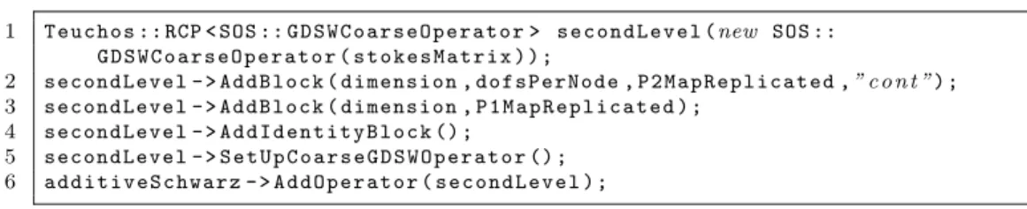
7.4. Setup of the coarse level. For the user interface of the coarse level setup, we refer to lines of code depicted in Figure 5. Each variable, i.e., velocity, pressure, and Lagrange multiplier, is added to the coarse space separately; see lines 2–5.
As described in section 6, we add one coarse basis function with Φ Γ,λ
0= 1,
that corresponds to the Lagrange multiplier, to the coarse space. Therefore, we use
1 T e u c h o s :: RCP < SOS :: G D S W C o a r s e O p e r a t o r > s e c o n d L e v e l (new SOS ::
G D S W C o a r s e O p e r a t o r ( s t o k e s M a t r i x ) ) ;
2 s e c o n d L e v e l - > A d d B l o c k ( d i m e n s i o n , d o f s P e r N o d e , P 2 M a p R e p l i c a t e d ,” c o n t ”) ; 3 s e c o n d L e v e l - > A d d B l o c k ( d i m e n s i o n , P 1 M a p R e p l i c a t e d ) ;
4 s e c o n d L e v e l - > A d d I d e n t i t y B l o c k () ;
5 s e c o n d L e v e l - > S e t U p C o a r s e G D S W O p e r a t o r () ; 6 a d d i t i v e S c h w a r z - > A d d O p e r a t o r ( s e c o n d L e v e l ) ;
Fig. 5. Second level setup of the two-level Schwarz preconditioner using the BlockMat for the Stokes matrix stokesMatrix; cf. subsection 7.2. The setup of the first level and the SumOperator additiveSchwarz is depicted in Figure 4. After adding both levels, additiveSchwarz corresponds to the monolithic GDSW preconditioner.
Communication Avg. apply 1st lvl. Avg. apply 2nd lvl.
Standard 1.42s 0.59s
Modified 1.28s 0.12s
Table 3
LDC Stokes problem in two dimensions with 4 096 subdomains; H/h = 160, δ = 16h. Timings for critical parts w.r.t. communication time of the two-level preconditioner with GDSW coarse problem. Standard communication uses Epetra Import and Epetra Export objects only. Modified communication uses additional communication; cf. subsection 7.4. ‘Avg. apply 1st lvl.’ and ‘Avg.
apply 2nd lvl.’ are times averaged over the number of iterations.
the method AddIdentityBlock() in line 4. The velocity and pressure variables are previously added using the AddBlock(), specifying, i.e., the dimension of the domain, number of degrees of freedom per node, and the ordering of the degrees of freedom in the system. The ordering options are “cont” (continuous), “sep” (separated), and
“user” (user defined). Continuous ordering corresponds to a nodewise ordering and separated ordering corresponds to dimensionwise ordering, whereas in the user defined ordering, Epetra Maps have to be provided by the user to define the ordering of the degrees of freedom. The Epetra Maps P2MapReplicated and P1MapReplicated correspond to the velocity and pressure index sets of the nonoverlapping subdomains, respectively. In combination with the ordering, these maps are used to identify the vertices, edges, and, in three dimensions, faces of the domain decomposition; see [36]
for a detailed description of this process.
For the computation of the discrete harmonic extensions, we extract the ma- trices A (i) II and A (i) IΓ , i = 1, ..., N, from A; since we assume that A is distributed according to the nonoverlapping subdomains, no communication is needed for this step. Now, we factorize each A (i) II in serial mode and solve −A (i) II φ (i) I = A (i) IΓ φ (i) Γ col- umn by column for φ (i) I ; cf. (14). Then, the global Blockmat φ is assembled. When SetUpCoarseGDSWOperator() is called, the coarse matrix is computed as A 0 = φ T Aφ and the resulting globally distributed coarse matrix is reduced to a smaller number of processes using multiple communication steps; cf. [36] for a more detailed discussion.
Here, we used three communication steps in all numerical results; in general, this led to the best total performance. Finally, if a direct coarse solver is used, the coarse matrix is factorized in serial or parallel mode.
7.5. Application of the preconditioner. Our global Epetra Map of the solu-
tion is uniquely distributed. Therefore, the Lagrange multiplier λ is assigned to only
one MPI rank although it belongs to each overlapping subdomain. Also, the coarse
basis function corresponding to the Lagrange multiplier couples all subdomains. Con-
Fig. 6. Structured (left) and unstructured (right) mesh and decomposition, H/h = 5.
sequently, the handling of the Lagrange multiplier in the monolithic preconditioners requires all-to-one and one-to-all communication. As already mentioned in [36], such communication patterns are, in general, not handled well by Epetra Export and Epetra Import objects. One way to overcome this issue is to introduce multiple communication steps. Here, we use MPI Broadcast and MPI Reduce for the commu- nication related to the Lagrange multiplier and Epetra Export and Epetra Import objects for the remaining degrees of freedom. In Table 3, we report the speed up due to separate communication of the Lagrange multiplier. We save 10% and 80%
time in each application of the first and second level, respectively, for the LDC Stokes problem in two dimensions on 4 096 MPI ranks.
Besides this, the application of the monolithic GDSW preconditioner is handled as for elliptic problems; cf. [36].
8. Numerical results. In this section, we present numerical results of our paral- lel implementation of the monolithic GDSW preconditioner. All parallel computations were carried out on the magnitUDE supercomputer at University Duisburg-Essen, Germany. A normal node on the magnitUDE has 64GB of RAM and 24 cores (Intel Xeon E5-2650v4 12C 2.2GHz), interconnected with Intel Omni-Path switches. Intel compiler version 17.0.1 and Intel MKL 2017 were used.
The two- and three-dimensional Navier-Stokes problems are solved with New- ton and Picard iteration, respectively, as we could not observe good convergence with Newton’s method without applying globalization techniques in three dimen- sions. Both methods are started with zero initial guess and the stopping criterion is kr nl (k) k/kr nl (0) k ≤ 10 −8 , with r nl (k) being the k-th nonlinear residual.
When using a direct solver for the coarse problem, we employ GMRES (General- ized minimal residual method) [58] for the solution of the linear systems. We use the stopping criterion kr (k) k ≤ εkr (0) k, where r (k) is the k-th unpreconditioned residual and ε = 10 −6 is the tolerance for Stokes and elasticity problems. For Navier-Stokes problems, we use the tolerance ε = 10 −4 for the linear systems. In case of inexact coarse solves, we employ Flexible GMRES (FGMRES) [57] for the outer iterations;
cf. subsection 8.1.3. For both Krylov methods, we use the implementations in the Trilinos package Belos. As a direct solver, we use MUMPS 5.1.1 through the Trilinos Amesos interface. The local problems are solved in serial mode, whereas in case of exact coarse solves, the coarse problems is solved in serial or parallel mode. For inex- act coarse solves, we iterate with GMRES up to a tolerance ε c . The number of MPI ranks for exact and inexact coarse solves is determined by the formula
(21) 0.5(1 + min{N umP rocs, max{N umRows/10 000, N umN onZeros/100 000}}),
where N umRows and N umN onZeros are the numbers of rows and nonzeros of A 0 ,
δ = 1h δ = 2h
N 4 9 16 25 36 49 64 4 9 16 25 36 49 64
#its. ˆ B
−1GDSW25 33 35 37 38 39 40 21 27 29 32 32 32 33
#its. ˆ B
−1P2−P121 25 27 28 28 29 29 18 29 21 22 22 22 22 Table 4
Iteration counts for LDC Stokes problem in two dimensions, varying number of subdomains N and overlap δ, H/h = 8. Stopping criterion ke
(k)k ≤ 10
−6, e
(k)= x
(k)− x
∗with reference solution x
∗.
# cores 64 256 1 024 4 096 8 100
# its. 66 70 69 68 67
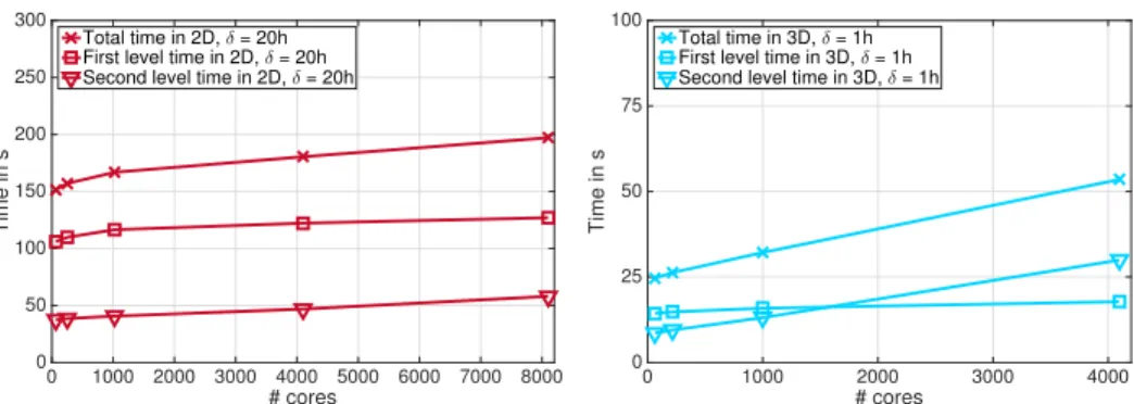
δ = 16h Time 154.7s 166.4s 172.9s 185.5 202.6s Effic. 98% 91% 88% 82% 75%
# its. 55 56 57 56 56
δ = 20h Time 151.7s 157.1s 166.9s 180.5 197.2 Effic. 100% 97% 91% 86% 77%
# its. 50 51 51 51 50
δ = 24h Time 156.6s 160.9s 169.7s 185.1s 199.4 Effic. 97% 94% 89% 82% 76%
Table 5
Iteration counts and weak scalability for two-dimensional LDC Stokes problem, H/h = 160, serial coarse solves. Baseline for the efficiency is the fastest time on 64 cores with overlap δ = 20h.
respectivly; cf. [36]. In our context, this formula tends to be dominated by the number of nonzeros. If not stated otherwise, we use above formula to determine the number of MPI ranks used in the coarse solution phase.
Unstructured meshes are constructed from structured meshes by moving the in- terior nodes; cf. Figure 6. To partition the unstructured meshes in parallel, we use ParMETIS 4.0.3 [44]. For the sake of clarity, we characterize all meshes and decompo- sitions by uniform parameters H and h throughout this section.
In the following numerical results, we report first level, second level, and total times. The first level time is the sum of construction and application time for the first level of the preconditioner, where the application is performed in every outer GMRES or FGMRES iteration. The total time is the sum of both levels.
8.1. Numerical results for Stokes problems. First, we present a comparison of monolithic Schwarz preconditioners with GDSW and standard Lagrangian coarse spaces; cf. subsections 5.1 and 5.2. Further, parallel scalability results for the mono- lithic GDSW preconditioner are presented for serial and parallel direct coarse solves and inexact coarse solves.
8.1.1. Comparison of Lagrangian and GDSW coarse spaces. Iterations counts for the solution of the LDC Stokes problem in two dimensions using mono- lithic Schwarz preconditioners with GDSW and Lagrangian coarse spaces are given in Table 4; the results were computed with Matlab on a structured meshes and do- main decompositions. GMRES terminates if the error e (k) = x (k) − x ∗ of the current iterate x (k) to the reference solution x ∗ of the linear system satisfies ke (k) k ≤ 10 −6 ; as reference solution we used the one obtained by a direct solver.
We observe that the performance of Lagrangian coarse spaces is slightly better
for structured domain decompositions. In contrast, the use of Lagrangian coarse
spaces for unstructured decompositions requires additional coarse triangulations and
0 1000 2000 3000 4000 5000 6000 7000 8000
# cores 0
50 100 150 200 250 300
Time in s
Total time in 2D, δ = 20h First level time in 2D, δ = 20h Second level time in 2D, δ = 20h
0 1000 2000 3000 4000
# cores 0
25 50 75 100
Time in s
Total time in 3D, δ = 1h First level time in 3D, δ = 1h Second level time in 3D, δ = 1h