A TLAS-CONF-2016-093 30 August 2016
ATLAS NOTE
ATLAS-CONF-2016-093
30th August 2016
Search for electroweak production of supersymmetric particles in final states with tau leptons in √
s = 13 TeV p p collisions with the ATLAS detector
The ATLAS Collaboration
Abstract
A search for the electroweak production of charginos and neutralinos in final states with at least two hadronically decaying tau leptons is presented. The analysis uses a dataset of proton–
proton collisions corresponding to an integrated luminosity of 14.8 fb − 1 , recorded with the ATLAS detector at the Large Hadron Collider at a centre-of-mass energy of
√ s = 13 TeV. No significant deviation from the Standard Model expectation is observed. Limits are derived in scenarios of ˜ χ +
1 χ ˜ −
1 pair production and ˜ χ ±
1 χ ˜ 0
2 and ˜ χ +
1 χ ˜ −
1 associated production. Common χ ˜ ±
1 - ˜ χ 0
2 masses up to 580 and 700 GeV respectively are excluded at 95 % confidence level assuming a massless ˜ χ 0
1 .
© 2016 CERN for the benefit of the ATLAS Collaboration.
Reproduction of this article or parts of it is allowed as specified in the CC-BY-4.0 license.
1 Introduction
Supersymmetry (SUSY) [1–7] adds a new symmetry to the Standard Model (SM) of particle physics, and postulates the existence of a super-partner, or sparticle , for each SM particle, whose spin differs by one half unit from the corresponding SM partner. In R -parity [8–12] conserving models, SUSY particles are always produced in pairs, and the lightest supersymmetric particle (LSP) is stable and provides a dark matter candidate [13–15].
In SUSY models, the electroweak sector contains charginos ( ˜ χ ± i , i = 1, 2), neutralinos ( ˜ χ 0 j , j = 1, 2, 3, 4 in order of increasing masses), and sleptons. Charginos and neutralinos are the mass eigenstates formed from the linear superpositions of the SUSY partners of the charged and neutral Higgs bosons and electroweak gauge bosons. The sleptons are the superpartners of the leptons and are referred to as left- or right-handed depending on the chirality of their SM partners. In this note only the ˜ χ ±
1 , the ˜ χ 0
2 , the ˜ χ 0
1 , and the scalar super-partner of the left-handed tau lepton (the stau, H τ ) and of the tau neutrino (the tau sneutrino, ˜ ν τ ) are assumed to be sufficiently light to be produced at the Large Hadron Collider (LHC) [16].
Models with light staus can lead to a dark matter relic density consistent with cosmological observations [17], and light sleptons in general could play a role in the co-annihilation of neutralinos [18,19]. Their mass is expected to be in the O (100 GeV) range in gauge-mediated [20–25] and anomaly-mediated [26, 27]
SUSY breaking models. Scenarios where the production of charginos, neutralinos, and sleptons may dominate at the LHC with respect to the production of squarks and gluinos can be realised in the general framework of the phenomenological Minimal Supersymmetric Standard Model (pMSSM) [28–30].
Simplified models [31–33] characterised by ˜ χ ±
1 χ ˜ 0
2 and ˜ χ +
1 χ ˜ −
1 production are considered in this note. In both simplified models the lightest neutralino is the LSP. The H τ and the ˜ ν τ are assumed to be lighter than the ˜ χ ±
1 and ˜ χ 0
2 . Charginos and neutralinos decay into the lightest neutralino via an intermediate on-shell stau or tau sneutrino, ˜ χ ±
1 → H τν( ν ˜ τ τ) → τν χ ˜ 0
1 , and ˜ χ 0
2 → H ττ → ττ χ ˜ 0
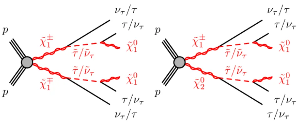
1 (see Figure 1).
The electroweak production of chargino pairs and associated production of chargino and next-to-lightest neutralinos are studied in final states with at least two hadronically decaying tau leptons and missing transverse momentum, using a dataset of
√ s = 13 TeV proton–proton collisions collected with the ATLAS detector in 2015 and 2016, with a combined integrated luminosity of 14.8 fb − 1 . In a previous search from the ATLAS collaboration [34], chargino masses up to 345 GeV were excluded at 95 % confidence level for a massless lightest neutralino in the scenario of direct production of wino-like chargino pairs. In the case of associated production of mass-degenerate charginos and next-to-lightest neutralinos, masses up to 410 GeV were excluded for a massless lightest neutralino. Recent results from the CMS collaboration on similar scenarios include Refs. [35, 36]. In Ref. [35], charginos lighter than 320 GeV are excluded at 95 % confidence level in the case of a massless lightest neutralino. The combined LEP limits on the stau1 and chargino2 masses are m
H τ > 87–93 GeV (depending on m
χ ˜ 0
1 ) and m χ ˜ ±
1 > 103 . 5 GeV [37–39].
1 The stau mass limit from LEP assumes gaugino mass unification, which is not assumed in the results presented here.
2 For the interval 0 . 1 . ∆m( χ ˜ ±
1 , χ ˜ 0
1 ) . 3 GeV, the chargino mass limit set by LEP degrades to 91 . 9 GeV.
˜ χ ± 1
˜ χ ∓ 1
˜ τ /˜ ν τ
˜ τ /˜ ν τ
p p
ν τ /τ τ /ν τ
˜ χ 0 1
ν τ /τ τ /ν τ
˜ χ 0 1
˜ χ ± 1
˜ χ 0 2
˜ τ /˜ ν τ
˜ τ /˜ ν τ
p p
ν τ /τ τ /ν τ
˜ χ 0 1
τ /ν τ τ /ν τ
˜ χ 0 1
Figure 1: Representative diagrams for the electroweak production processes of supersymmetric particles considered in this work: (left) ˜ χ +
1 χ ˜ −
1 and (right) ˜ χ ±
1 χ ˜ 0
2 production.
2 The ATLAS detector
The ATLAS detector [40] is a multi-purpose particle physics detector with forward-backward symmetric cylindrical geometry, and nearly 4 π coverage in solid angle3. It features an inner tracking detector (ID) surrounded by a 2 T superconducting solenoid, electromagnetic and hadronic calorimeters, and a muon spectrometer (MS). The ID covers the pseudorapidity region |η| < 2 . 5 and consists of a silicon pixel detector, a silicon microstrip detector, and a transition radiation tracker. One significant upgrade for the
√ s = 13 TeV running period is the presence of the Insertable B-Layer [41], an additional pixel layer close to the interaction point, which provides high-resolution hits at small radius to improve the tracking performance. The calorimeters are composed of high-granularity liquid-argon (LAr) electromagnetic calorimeters with lead, copper, or tungsten absorbers (in the pseudorapidity region |η | < 3 . 2) and a steel–scintillator hadronic calorimeter (over |η | < 1 . 7). The end-cap and forward regions, spanning 1 . 5 < |η | < 4 . 9, are instrumented with LAr calorimeters for both the electromagnetic and hadronic measurements. The MS surrounds the calorimeters and consists of three large superconducting air-core toroid magnets, each with eight coils, a system of precision tracking chambers ( |η | < 2 . 7), and detectors for triggering ( |η | < 2 . 4). A two-level trigger system is used to sample events [42].
3 Data and simulated event samples
The analysed dataset, after the application of beam, detector and data quality requirements, corresponds to an integrated luminosity of 14.8 fb − 1 of p – p collision data recorded in 2015 and 2016 at
√ s = 13 TeV with the ATLAS detector. The preliminary uncertainty on the combined 2015+2016 integrated luminosity is 2.9 %. It is derived, following a methodology similar to that detailed in Refs. [43] and [44], from a preliminary calibration of the luminosity scale using x − y beam-separation scans performed in May 2016.
3 ATLAS uses a right-handed coordinate system with its origin at the nominal interaction point (IP) in the centre of the detector, and the z -axis along the beam line. The x -axis points from the IP to the centre of the LHC ring, and the y -axis points upwards.
Cylindrical coordinates (r, φ) are used in the transverse plane, φ being the azimuthal angle around the z -axis. Observables
labelled transverse refer to the projection into the x– y plane. The pseudorapidity is defined in terms of the polar angle θ by
η = − ln tan (θ/ 2 ) . The rapidity is defined as y = 0 . 5 ln[ (E + p z )/(E − p z ) ], where E is the energy and p z the longitudinal
momentum of the object of interest.
Monte Carlo (MC) simulated event samples are used to estimate the SUSY signal yields and to aid in evaluating the SM backgrounds. Events with Z /γ ∗ → `` (` = e, µ, τ) and W → `ν produced with accompanying jets (including light and heavy flavours) are generated at next-to-leading order (NLO) in the strong coupling constant with Sherpa 2.2.0 [45, 46]. Matrix elements (MEs) are calculated for up to two partons at NLO and four partons at leading order (LO). The MEs are calculated using the Comix [47] and OpenLoops [48] generators and merged with the Sherpa 2.2.0 parton shower [49] using the ME+PS@NLO prescription [46]. The NNPDF3.0NNLO [50] particle distribution function (PDF) set is used in conjunction with a dedicated parton-shower tuning developed by the Sherpa authors. The W /Z +jets events are normalised to their next-to-next-to-leading order (NNLO) cross sections. A simplified scale setting prescription has been used in the multi-parton MEs, to improve the event generation speed.
A theory-based reweighting of the jet multiplicity distribution is applied at event level, derived from event generation with the strict scale prescription.
The diboson samples ( V V = W W/W Z/Z Z ) are generated using Sherpa 2.1 with the CT10 PDF set [51].
The fully leptonic diboson processes are simulated including final states with all possible combinations of charged leptons and neutrinos. The MEs contain all diagrams with four electroweak vertices, and they are calculated for up to one parton (4 ` , 2 ` +2 ν , Z Z , W W ) or no additional partons (3 ` +1 ν , 1 ` +3 ν , W Z ) at NLO and up to three partons at LO. Each of the diboson processes is normalised to the corresponding NLO cross-section [52].
The production of top quark pairs and single top quarks in the W t and s -channels is generated with Powheg-Box r3026 [53], with the CT10 PDF set and the Perugia2012 [54] set of tuned parameters of the Monte Carlo programs (tune). Parton fragmentation and hadronisation are simulated with Pythia 6.428 [55]. The modelling of heavy-flavour decays is improved using EvtGen 1.2.0 [56]. The overall cross section is normalised to NNLO including resummation of next-to-next-to-leading logarithmic (NNLL) soft gluon terms [57] for t¯ t , to NLO+NNLL accuracy for single-top-quark W t -channel [58], and to NLO for the t - and s -channels [59]. Top-antitop quark production with an additional W or Z boson is generated using MadGraph v2.2.2 [60], fragmentation and hadronisation are simulated with Pythia 8.186 [61].
The ATLAS underlying-event tune A14 [62] is used with the NNPDF2.3LO [63] PDF set, the cross sections are normalised to NLO accuracy [64, 65].
Simulated signal samples are generated using MadGraph5_aMC@NLO v2.2.3 interfaced to Pythia 8.186 with the A14 tune for the modelling of the parton showering (PS), hadronisation and underlying event.
The ME calculation is performed at tree-level and includes the emission of up to two additional partons.
The PDF set used for the generation is NNPDF2.3LO. The ME–PS matching is done using the CKKW- L [66] prescription, with a matching scale set to one quarter of the mass of the pair of produced particles.
Signal cross sections are calculated to next-to-leading order in the strong coupling constant, adding the resummation of soft gluon emission at next-to-leading-logarithmic accuracy (NLO+NLL) [67–69]. The nominal cross section and the uncertainty are taken from an envelope of cross-section predictions using different PDF sets and factorisation and renormalisation scales, as described in Ref. [70].
Two simplified models characterised by ˜ χ ±
1 χ ˜ 0
2 and ˜ χ +
1 χ ˜ −
1 production are considered. In these models, all sparticles other than ˜ χ ±
1 , ˜ χ 0
2 , ˜ χ 0
1 , ˜ τ L and ˜ ν τ are assumed to be heavy (masses of order of 2 TeV). The neutralinos and charginos decay via intermediate staus and tau sneutrinos. The stau and tau sneutrino are assumed to be mass-degenerate. The mass of the ˜ τ L state is set to be halfway between those of the ˜ χ ±
1 and the ˜ χ 0
1 . The ˜ χ 0
1 is purely bino. In the model characterised by ˜ χ ±
1 χ ˜ 0
2 production, ˜ χ ±
1 and ˜ χ 0
2 are assumed to be pure wino and mass-degenerate, whereas in the model where only ˜ χ +
1 χ ˜ −
1 production is considered, the ˜ χ 0
2 is assumed to have a mass of the order of 2 TeV. In both models, the ˜ χ ±
1 mass is varied between 100
and 800 GeV, and the ˜ χ 0
1 mass is varied between zero and 350 GeV. The cross section for ˜ χ ±
1 χ ˜ 0
2 ( ˜ χ +
1 χ ˜ −
1 ) production ranges from 23 (11.6) pb for a ˜ χ ±
1 mass of 100 GeV to 4.8 (2.2) fb for a ˜ χ ±
1 mass of 800 GeV.
The direct production of stau pairs is not considered due to the low cross section of this process compared to that of ˜ χ ±
1 χ ˜ 0
2 and ˜ χ +
1 χ ˜ −
1 production.
Two reference points are used throughout this paper to illustrate the typical features of the SUSY models to which this analysis is sensitive:
• Reference point 1: simplified model for chargino–neutralino production with mass of ˜ χ ±
1 and ˜ χ 0
2
equal to 400 GeV, and massless ˜ χ 0
1 ;
• Reference point 2: simplified model for chargino–chargino production with mass of ˜ χ ±
1 equal to 400 GeV, and massless ˜ χ 0
1 .
SM samples are processed through a detailed detector simulation [71] based on Geant 4 [72], whereas SUSY samples are passed through a fast detector simulation based on a parametrisation of the performance of the ATLAS electromagnetic and hadronic calorimeters [73]. All MC samples are reconstructed using the same algorithms as the data. The effect of multiple proton–proton collisions in the same or nearby bunch crossings is also taken into account.
4 Event and object reconstruction
Events with at least one reconstructed primary vertex [74] are selected. A primary vertex must have at least two associated charged-particle tracks with transverse momentum p T > 400 MeV and be consistent with the beam spot envelope. If there are multiple primary vertices in an event, the one with the largest P p 2
T of the associated tracks is chosen.
Jets are reconstructed from three-dimensional calorimeter energy clusters [75] using the anti- k t al- gorithm [76, 77] with a radius parameter of 0.4. Jet energies are corrected for detector inhomogeneities, the non-compensating nature of the calorimeter, and the impact of pile-up, using factors derived from test beam and proton–proton collision data, and from a detailed Geant 4 detector simulation [78, 79]. The impact of pile-up is accounted for by using a technique, based on jet areas, that provides an event-by-event and jet-by-jet correction [80]. Events containing jets that are likely to have arisen from detector noise or cosmic rays are removed. For this analysis jets are required to have p T > 20 GeV and |η | < 2 . 8. To suppress jets from simultaneous pp interactions, jets with p T < 60 GeV and |η | < 2 . 4 are required to have a jet-vertex-tagger [81] output larger than 0 . 59, indicating that a significant fraction of their associated tracks is originating from the primary vertex.
Jets containing b -hadrons ( b -jets) are identified using the MV2c10 algorithm, a multivariate discriminant making use of track impact parameters and reconstructed secondary vertices [82]. Candidate b -jets are required to have p T > 20 GeV and |η | < 2 . 5. A working point with an average b -tagging efficiency of 77 % for simulated t¯ t events is used [83, 84]. The rejection factors for light-quark jets, c -quark jets and hadronically decaying tau leptons are approximately 134, 6 and 55, respectively. Corrections needed to correctly model jets tagged as b -jets are included.
Electron candidates are reconstructed by matching clusters in the electromagnetic calorimeter with charged
particle tracks in the inner detector. Electrons are required to have p T > 10 GeV, |η| < 2 . 47, and to satisfy
the ‘loose’ working point according to a likelihood-based identification [85], with an additional requirement
on the hits in innermost pixel layer. Muon candidates are identified by matching an extrapolated inner detector track and one or more track segments in the muon spectrometer. Muons are required to have p T > 10 GeV and |η | < 2 . 4 and fulfil ‘medium’ quality criteria [86]. Events containing a muon candidate with a poorly measured charge-to-momentum ratio ( σ(q/p) / |q/p| > 0 . 2) are rejected. Events are required not to contain any candidate muon with high impact parameters ( |z 0 | > 1 mm or |d 0 | > 0 . 2 mm), as these may originate from cosmic rays. The efficiencies for electrons and muons to satisfy the reconstruction, identification and isolation criteria are measured in samples of Z and J/ψ leptonic decays, and corrections are applied to the simulated samples to reproduce the efficiencies in data.
The reconstruction of hadronically decaying taus is based on the information from tracking in the ID and three-dimensional clusters in the electromagnetic and hadronic calorimeters. The tau reconstruction algorithm is seeded by jets reconstructed as described above but with p T > 10 GeV and |η | < 2 . 47.
The reconstructed energies of the hadronically decaying tau candidates are corrected to the tau energy scale, which is calibrated using tau-energy-scale corrections based on simulation. The latter are derived independently from jet-energy-scale corrections. Tau neutrinos from the tau lepton decay are not taken into account in the reconstruction and calibration of the tau energy and momentum. Since taus decay mostly to either one or three charged pions, together with a neutrino and often additional neutral pions, tau candidates are required to have one or three associated charged particle tracks (prongs) and the total electric charge of those tracks must be ± 1 times the electron charge. To improve the discrimination between hadronically decaying taus and jets, electrons, or muons, multivariate algorithms are used [87]. The tau identification algorithm used in this analysis is based on the Boosted Decision Tree (BDT) method. The BDT algorithms use as input various track and cluster variables to discriminate taus from jets. For 1-prong (3-prong) taus the signal efficiencies are 60 % and 55 % (50 % and 40 %) for the ‘loose’ and ‘medium’ working points, respectively. In the following, tau candidates are required to pass the medium identification criteria for jet discrimination (‘medium’ taus), unless otherwise stated. For electron discrimination, an overlap-based veto is used. This requirement has about 95 % efficiency, and a rejection factor from 10 to 50 depending on the η range. Tau candidates are required to have p T > 20 GeV and |η | < 2 . 47, excluding the transition region between the barrel and end-cap calorimeters (1 . 37 < |η | < 1 . 52).
The simulation is corrected for differences in the efficiency of the tau identification and trigger algorithms between data and simulation. For hadronically decaying taus coming from prompt boson decays, the corrections are calculated with a tag-and-probe method in a sample of Z → ττ events where one tau decays hadronically and the other leptonically into a muon and two neutrinos [88].
The measurement of the missing transverse momentum vector, p miss
T , and its magnitude, E miss
T , is based on the vectorial sum of the p T of reconstructed objects (jets, taus, electrons, photons, muons) and an additional soft term. The soft term is constructed from all tracks that are not associated with any physics object, and that are associated to the primary vertex. In this way, the missing transverse momentum is adjusted for the best calibration of the jets and the other identified physics objects, while maintaining pileup independence in the soft term [89, 90].
The possible double counting of reconstructed objects is resolved in the following order. Tau candidates close to electron or muon candidates ( ∆R < 0 . 2, where ∆R = p
(∆y) 2 + (∆φ) 2 ) are removed, as are
electrons sharing a track with a muon. For electrons close to a jet ( ∆R < 0 . 4), the electron is removed,
except when ∆R < 0 . 2 and the jet is not b -tagged, in which case the jet is removed. Any remaining jet
within ∆R < 0 . 4 of a muon or tau lepton is removed.
5 Event selection
The events used in this analysis are recorded using a combined ditau + E miss T trigger requiring the identification of two hadronically decaying tau candidates with p T exceeding 35 (25) GeV for the leading (next-to-leading) tau candidate, and E miss
T of at least 50 GeV. The efficiency of each leg of the ditau trigger is measured using a sample of Z → ττ events where one tau decays hadronically and the other leptonically into a muon and two neutrinos. The single tau trigger efficiency for correctly identified tau leptons reaches a constant value ( ∼ 90 %) when the leading tau candidate has p T > 50 GeV and the next-to-leading tau candidate has p T > 40 GeV.
Events are required to have at least two tau candidates with opposite electrical charge. The ditau invariant mass of any opposite-sign (OS) pair must be larger than 12 GeV to remove taus from low-mass resonances.
This requirement has negligible effect on the signal efficiency. Two of the reconstructed taus must have fired the ditau part of the trigger, and satisfy the p T requirements to be in the region where the trigger efficiency is constant. To work in the region where the E miss
T part of the trigger reaches full efficiency, events are selected by requiring E miss
T > 150 GeV.
To enhance the sensitivity to the SUSY signal and suppress SM backgrounds, additional requirements are applied that define the so-called signal regions (SR). To reject events from SM processes containing a top quark, selected events must not contain any b -jet ( b-jet veto ). To suppress SM backgrounds with a Z boson, events are selected by requiring that the reconstructed invariant mass of all oppositely charged tau pairs must not be within 10 GeV of the visible Z boson mass4 (79 GeV). This requirement is referred to as the Z -veto .
The variable that has the highest discrimination power between SM processes and the SUSY signals of interest is the stransverse mass m T2 [91, 92]. It is defined as:
m T2 = min
q T
f max
m T ,τ 1 (p T ,τ 1 , q T ), m T ,τ 2 (p T ,τ 2 , p miss
T − q T ) g ,
where p T ,τ 1 and p T ,τ 2 are the transverse momenta of the two taus, and q T is the transverse vector that minimises the larger of the two transverse masses m T ,τ 1 and m T ,τ 2 . The latter is defined by
m T (p T , q T ) = p
2 ( p T q T − p T · q T ).
In events where more than two tau candidates are selected, m T2 is computed among all possible tau pairs and the combination leading to the largest value is chosen. For t¯ t and W W events, in which two W bosons decay leptonically and p miss
T is the sum of the transverse momenta of the two neutrinos, the m T2 distribution has a kinematic end-point at the W mass. For large mass differences between the next-to- lightest neutralinos, the charginos, or the staus and the lightest neutralino, the m T2 distribution for signal events extends significantly beyond the distributions of the t t ¯ and W W events.
Two SRs5 based on large m T2 and E miss
T requirements are defined in this analysis. Both SRs have been optimised to improve the sensitivity to signal models with charginos heavier than 400 GeV and massless LSP. SR-C1N2 targets chargino-neutralino production, where up to three taus are expected in the final state. SR-C1N2 is therefore defined by the requirement of having events with at least two hadronically reconstructed taus, and it is inclusive in the number of additional leptons of any flavour. SR-C1C1 targets
4 The visible Z boson mass is measured using the mean value of a gaussian fit of the reconstructed invariant mass distribution of OS tau pairs in a MC sample of Z → ττ events with associated jets.
5 In the SR definitions, the following mnemonic naming conventions are used: C1 stands for ˜ χ ±
1 , and N2 for ˜ χ 0
2 .
chargino-chargino production, where two taus are expected in the final state. SR-C1C1 is defined exactly as SR-C1N2, except that events containing additional light leptons (candidate electrons or muons after resolving the overlap between the various reconstructed objects as described in Section 4) are vetoed ( light lepton veto ). The requirements for each SR are summarised in Table 1. The two SRs are not mutually exclusive.
Table 1: Signal region definitions.
SR-C1C1 SR-C1N2
light lepton veto - at least two medium taus at least one opposite sign tau pair
b -jet veto Z -veto E miss
T > 150 GeV m T2 > 70 GeV
6 Standard Model background estimation
The main SM processes contributing to the selected final states are multi-jet, W +jets and diboson pro- duction. Background events may contain a combination of ’real’ taus, defined as correctly identified tau leptons, or ’fake’ taus, which can originate from a misidentified light-flavour quark or gluon jet, an electron or a muon.
In multi-jet events nearly all tau candidates are misidentified jets. Due to the large cross section and the fact that modelling the tau misidentification rate from jets in MC is challenging, the multi-jet contribution in the SRs is estimated from data, as described in Section 6.1. The contribution arising from heavy-flavour multi-jet events containing a real tau lepton from the heavy-flavour quark decay is included in the multi-jet estimate. The contribution of W +jets events, which contain one real tau from the W decay and one or more misidentified jets, is estimated from MC simulation, and normalised to data in a dedicated control region, as described in Section 6.2.
Diboson production contributes mainly with events containing real tau leptons coming from W W and Z Z decaying into a ττνν final state. Additional SM backgrounds arise from Z +jets production, or events that contain a top quark or top-quark pair in association with jets or additional W or Z bosons (collectively referred to as top background in the following). The contribution from real taus exceeds 90 % in Z +jets and diboson production, and ranges from 45 % to 75 % in backgrounds containing top quarks. The contribution of fake taus from heavy-flavour decays in jets is negligible. To estimate the irreducible background, which includes diboson, Z +jets and top quark events, only MC simulated samples are used, as described in Section 6.3.
The sources of systematic uncertainty on the background estimates are described in Section 7. Finally,
for each signal region, a simultaneous fit based on the profile likelihood method [93] is performed to
normalise the multi-jet and W +jets background estimates, as described in Section 8.
6.1 Multi-jet background estimation
One of the dominant backgrounds in the SRs originates from jets misidentified as tau leptons in multi-jet production. This contribution is estimated from data using the ABCD method. Four exclusive regions, labelled as A, B, C (the control regions, CR) and D (the SR), are defined in a two-dimensional plane as a function of two (or more) uncorrelated discriminating variables. In this case, the ratio of events in the control regions CR-C and -B equals to that in SR-D and CR-A: the number of events in the SR-D, N D , can therefore be calculated from that in CR-A, N A , multiplied by the transfer factor T = N C /N B . The tau identification criterion (tau-id) based on the jet BDT quality requirement, the charge of the two taus, the invariant mass of the two taus, and the kinematic variables m T2 and E miss
T are used as discriminating variables to define CR-A, CR-B, CR-C and SR-D.
The CR-A and the SR-D are defined in the same way except that in CR-A the taus are required to have same sign (SS) electrical charge, and to pass the loose jet BDT requirement (‘loose’ taus). Events with invariant mass of the two taus larger than 200 GeV are rejected to suppress the signal contamination in CR-A. The signal contamination in CR-A is negligible in ˜ χ +
1 χ ˜ −
1 production and ranges from a few percent to 60 % for ˜ χ ±
1 χ ˜ 0
2 production for most of the (m χ ˜ ±
1 , m
χ ˜ 0 1
) region, except for the already excluded region [34] at low χ ˜ +
1 ( ˜ χ 0
2 ) and ˜ χ 0
1 masses, where it goes up to almost 100 %. The signal contamination in the CR-A is taken into account in the simultaneous fit described in Section 8.
The same requirement on the tau-id and the charge of the two taus as in CR-A (SR-D) is applied in CR-B (CR-C). In CR-B and CR-C, less stringent requirements on the kinematic variables m T2 and E miss
T are
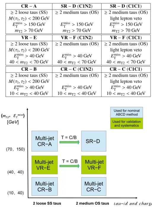
applied. Furthermore, two validation regions (VR), VR-E and VR-F are defined. The VR-E (VR-F) has the same definition as the CR-A (SR-D) except for intermediate requirements on the kinematic variables. The validation regions are used to verify the extrapolation of the ABCD estimation to the SR-D, and to estimate the systematic uncertainty from the residual correlation between the tau-id, the charge requirement, and the kinematic variable. Two sets of VRs are defined, corresponding to the two SRs, SR-C1N2 and SR-C1C1 defined in Section 5. The definitions of the control and validation regions are summarised in Table 2. The regions A–F are drawn schematically in Figure 2.
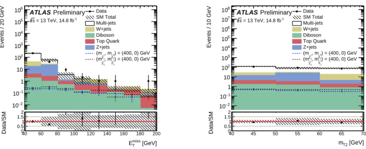
The number of multi-jet events in the control and validation regions is estimated from data after subtraction of other SM contributions estimated from MC simulation. In CR-B and VR-E more than 90 % of the events come from multi-jet production. In CR-A and CR-C the multi-jet purity is larger than 68 % and 75 %, respectively. Good agreement between data and SM backgrounds is found in VR-F, as shown in Figure 3.
6.2 W +jets background estimation
The production of W +jets events with at least one misidentified tau is an important background in the
SRs, making up for about 11 % of the expected SM background. A dedicated control region ( W -CR) is
used to normalise the W +jets MC estimation to data. The W -CR is enriched in events where the W decays
leptonically into a muon and a neutrino to suppress multi-jet contamination. Events are selected with a
single-muon trigger, using the lowest unprescaled p T thresholds available. Events containing exactly one
isolated muon and one candidate tau with opposite electrical charge are selected. The muon is required to
have p T > 30 GeV. In addition, an isolated muon must satisfy ‘GradientLoose’ [94] isolation requirements,
which rely on the use of tracking-based and calorimeter-based variables and implement a set of η - and
p T -dependent criteria. The distance of closest approach in the transverse plane of an isolated muon to
Table 2: The multi-jet control region and validation region definitions. The b -jet and Z vetoes are applied to all regions.
CR − A SR − D (C1N2) SR − D (C1C1)
≥ 2 loose taus (SS) ≥ 2 medium taus (OS) ≥ 2 medium taus (OS) M (τ 1 , τ 2 ) < 200 GeV light lepton veto
E miss
T > 150 GeV E miss
T > 150 GeV E miss
T > 150 GeV m T2 > 70 GeV m T2 > 70 GeV m T2 > 70 GeV
VR − E VR − F (C1N2) VR − F (C1C1)
≥ 2 loose taus (SS) ≥ 2 medium taus (OS) ≥ 2 medium taus (OS) M (τ 1 , τ 2 ) < 200 GeV light lepton veto
E miss
T > 40 GeV E miss
T > 40 GeV E miss
T > 40 GeV 40 < m T2 < 70 GeV 40 < m T2 < 70 GeV 40 < m T2 < 70 GeV
CR − B CR − C (C1N2) CR − C (C1C1)
≥ 2 loose taus (SS) ≥ 2 medium taus (OS) ≥ 2 medium taus (OS) M (τ 1 , τ 2 ) < 200 GeV light lepton veto
E miss
T > 40 GeV E miss
T > 40 GeV E miss
T > 40 GeV 10 < m T2 < 40 GeV 10 < m T2 < 40 GeV 10 < m T2 < 40 GeV
tau-id and charge
( m T2 , E T miss ) [GeV]
Multi-jet VR−E
Multi-jet VR−F
Used for validation and systematics
2 loose SS taus 2 medium OS taus
Multi-jet CR−A
Used for nominal ABCD method
Multi-jet
CR−B Multi-jet
CR−C SR−D
T = C/B
T = C/B (70,150)
(40,40)
(10,40)
Figure 2: Illustration of the ABCD method for the multi-jet background determination. The control regions A, B, C, and signal region D for the ABCD method described in the text (labelled as Multi-jet CR-A/B/C and SR-D) are drawn as light blue boxes. Shown in green and labelled as Multi-jet-VR are the regions E and F, which are used to validate the ABCD method and to estimate the systematic uncertainties.
the event primary vertex must be within three standard deviations from its measurement in the transverse
plane. The longitudinal impact parameter of an isolated muon, z 0 , must satisfy |z 0 sin θ| < 0 . 5 mm. The
tau candidate must pass the medium jet BDT and is required to have p T > 40 GeV.
[GeV]
m
T240 60 80 100 120 140 160 180 200
Events / 20 GeV
−2
10
−1
10 1 10 10
210
310
410
510
6Data
SM Total Multi-jets W+jets Diboson Top Quark Z+jets
) = (400, 0) GeV
0 χ∼2
±
, m
χ∼1
(m
) = (400, 0) GeV
± χ∼1
±
, m
χ∼1
(m = 13 TeV, 14.8 fb
-1s
Preliminary ATLAS
[GeV]
miss
E
T40 60 80 100 120 140 160 180 200
Data/SM
0 0.5 1 1.5 2[GeV]
m
T240 45 50 55 60 65 70
Events / 10 GeV
−2
10
−1
10 1 10 10
210
310
410
510
610
710
8Data
SM Total Multi-jets W+jets Diboson Top Quark Z+jets
) = (400, 0) GeV
0 χ∼2
±
, m
χ∼1
(m
) = (400, 0) GeV
± χ∼1
±
, m
χ∼1
(m = 13 TeV, 14.8 fb
-1s
Preliminary ATLAS
[GeV]
m
T240 45 50 55 60 65 70
Data/SM
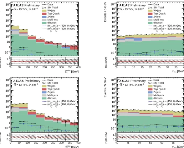
0 0.5 1 1.5 2Figure 3: The E miss
T (left) and m T2 (right) distributions in the multi-jet background VR-F (C1N2) defined in Table 2. The stacked histograms show the contribution of the non-multi-jet SM backgrounds from MC simulation, normalised to 14.8 fb − 1 . The multi-jet contribution is estimated from data using the ABCD method. The hatched bands represent the combined statistical and systematic uncertainties on the sum of the SM backgrounds shown. For illustration, the distributions of the SUSY reference points (defined in Section 3) are also shown as dashed lines.
The contribution from events with top quarks is suppressed by rejecting events containing b -tagged jets.
To suppress multi-jet and Z +jets events, requirements on E miss
T , m T ,µ , and m T ,τ + m T ,µ are applied. Events in the W -CR are selected by requiring low m T2 , while the high m T2 region is used to validate the W +jets estimate ( W validation region, W -VR). The definitions of the W -CR and W -VR are given in Table 3.
The multi-jet contribution in the W -CR (-VR) is estimated by counting the number of events in data satisfying the same requirements as the W -CR (-VR) but with same-sign (SS) charge of the two leptons.
Events from SM processes other than multi-jet production are subtracted from the data counts in the SS region, using their MC prediction. The OS–SS method relies on the fact that in the multi-jet background the ratio of SS to OS events is close to unity, whilst a significant difference from unity is expected for W +jets production. The latter is dominated by gu/gd -initiated processes that often give rise to a jet originating from a quark, the charge of which is anti-correlated with the W -boson charge.
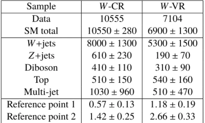
The event yields in the W -CR and W -VR are given in Table 4. The purity of the selection in W +jets events is around 76 % (78 %) in the W -CR (VR). Good agreement between data and SM predictions is observed.
The signal contamination in the W -CR and W -VR is negligible. Distributions of the kinematic variables defining the SRs are shown in Figure 4.
Table 3: The W -CR (left) and W -VR (right) definition.
W -CR W -VR
one isolated muon and one medium tau with opposite sign b -jet veto
E miss
T > 20 GeV m T,µ > 50 GeV m T,µ + m T,τ > 80 GeV
m T2 < 40 GeV 40 GeV < m T2 < 70 GeV
Table 4: Event yields in the W -CR and W -VR. The SM backgrounds other than multi-jet production are estimated from MC simulation and normalised to 14.8 fb − 1 . The contribution of W +jets events is scaled with the normalisation factor obtained from the fit described in Section 8. The multi-jet contribution is estimated from data using the OS–SS method. The shown uncertainties are the sum in quadrature of statistical and systematic uncertainties. The correlation of systematic uncertainties among control and validation regions and background processes, in particular the major correlations in the W+jets and multi-jet estimation due to OS–SS techniques, is fully taken into account in the fit.
Sample W -CR W -VR
Data 10555 7104
SM total 10550 ± 280 6900 ± 1300 W +jets 8000 ± 1300 5300 ± 1500
Z +jets 610 ± 230 190 ± 70
Diboson 410 ± 110 310 ± 90
Top 510 ± 150 540 ± 160
Multi-jet 1030 ± 960 510 ± 470 Reference point 1 0 . 57 ± 0 . 13 1 . 18 ± 0 . 19 Reference point 2 1 . 42 ± 0 . 25 2 . 66 ± 0 . 33
6.3 Irreducible background estimation
Irreducible SM backgrounds arise mainly from t t ¯ , single top, t¯ t + V , Z/γ ∗ +jets and diboson ( W W , W Z and Z Z ) processes and are estimated with MC simulation. Other SM backgrounds are negligible. The diboson background mainly arises from W W → τντν and Z Z → ττνν events, in which more than 96 % contribution is from two real tau leptons with good MC modeling.
The inclusive contribution from t¯ t , single top, t t ¯ + V and Z/γ ∗ +jets amounts to about 12–15 % of the total background in the signal regions. The MC estimates are validated in regions enriched in Z/γ ∗ +jets and top events. For both regions, events are recorded using the ditau + E T miss trigger. Events are required to have at least two tau candidates with opposite electrical charge. In the Z/γ ∗ +jets validation region ( Z -VR) at least two tau candidates must satisfy the medium jet BDT quality requirement. To suppress top backgrounds, events containing b -jets are vetoed. To further enhance the purity of Z/γ ∗ +jets events, events are selected by requiring low m T2 . In the top-quark validation region (Top-VR) at least one tau candidate must satisfy the medium jet BDT quality requirement. To increase the contribution from top events, events must contain at least one b -tagged jet with p T > 20 GeV, and the events should be kinematically compatible with t¯ t production (top-tagged) through the use of the variable m CT [95]. The scalar sum of the p T of the two taus and of at least one combination of two jets in an event must exceed 100 GeV. Top-tagged events are required to possess m CT values calculated from combinations of jets and taus consistent with the expected bounds from t t ¯ events as described in Ref. [96]. The Z -VR and Top-VR requirements are summarized in Table 5.
The purity of the selection in Z +jets and t t ¯ events is above 80 % in the respective validation regions and
good agreement between the data and SM expectation is observed. The m T2 distribution in the Z -VR and
Top-VR is shown in Figure 5.
0 50 100 150 200 250 300 350 400
Events / 50 GeV
−1
10 1 10 10
210
310
410
510
610
710
8Data
SM Total W+jets Top Quark Z+jets Multi-jets diboson
) = (400, 0) GeV
0 χ∼2
±
, m
χ∼1
(m
) = (400, 0) GeV
± χ∼1
±
, m
χ∼1
(m = 13 TeV, 14.8 fb
-1s
Preliminary ATLAS
[GeV]
miss
E
T0 50 100 150 200 250 300 350 400
Data/SM
0.5 0 1
1.5 2 0 5 10 15 20 25 30 35 40
Events / 5 GeV
−1
10 1 10 10
210
310
410
510
610
710
810
910
10Data
SM Total W+jets Top Quark Z+jets Multi-jets diboson
) = (400, 0) GeV
0 χ∼2
±
, m
χ∼1
(m
) = (400, 0) GeV
± χ∼1
±
, m
χ∼1
(m = 13 TeV, 14.8 fb
-1s
Preliminary ATLAS
[GeV]
m
T20 5 10 15 20 25 30 35 40
Data/SM
0.5 0 1 1.5 2
0 50 100 150 200 250 300 350 400
Events / 50 GeV
−1
10 1 10 10
210
310
410
510
610
710
8Data
SM Total W+jets Top Quark Z+jets Multi-jets diboson
) = (400, 0) GeV
0 χ∼2
±
, m
χ∼1
(m
) = (400, 0) GeV
± χ∼1
±
, m
χ∼1
(m = 13 TeV, 14.8 fb
-1s
Preliminary ATLAS
[GeV]
miss
E
T0 50 100 150 200 250 300 350 400
Data/SM
0.5 0 1
1.5 2 40 45 50 55 60 65 70
Events / 5 GeV
−1
10 1 10 10
210
310
410
510
610
710
810
910
10Data
SM Total W+jets Top Quark Z+jets Multi-jets diboson
) = (400, 0) GeV
0 χ∼2
±
, m
χ∼1
(m
) = (400, 0) GeV
± χ∼1
±
, m
χ∼1
(m = 13 TeV, 14.8 fb
-1s
Preliminary ATLAS
[GeV]
m
T240 45 50 55 60 65 70
Data/SM
0.5 0 1 1.5 2
Figure 4: The E miss
T (left) and m T2 (right) distributions in the W -CR (top) and W -VR (bottom). The SM backgrounds other than multi-jet production are estimated from MC simulation and normalised to 14.8 fb − 1 . The contribution of W +jets events is scaled with the normalisation factor obtained from the fit described in Section 8. The multi-jet contribution is estimated from data using the OS–SS method. The hatched bands represent the combined statistical and systematic uncertainties on the total SM background. For illustration, the distributions of the SUSY reference points (defined in Section 3) are also shown as dashed lines. The lower panels show the ratio of data to the SM background estimate.
Table 5: The Z -VR (left) and Top-VR (right) validation region definition.
Z -VR Top-VR
at least two medium taus at least one medium and one loose tau at least one opposite sign tau pair
b -jet veto at least 1 b -jet
m T2 < 20 GeV m CT top-tagged
0 2 4 6 8 10 12 14 16 18 20
Events / 5 GeV
−2
10
−1
10 1 10 10
210
310
410
510
6Data
SM Total Z+jets W+jets Top Quark diboson
) = (400, 0) GeV
0 χ∼2
±
, m
χ∼1
(m
) = (400, 0) GeV
± χ∼1
±
, m
χ∼1
(m = 13 TeV, 14.8 fb
-1s
Preliminary ATLAS
[GeV]
m
T20 2 4 6 8 10 12 14 16 18 20
Data/SM
0.5 0 1
1.5 2 0 20 40 60 80 100 120 140 160 180 200
Events / 40 GeV
−2
10
−1
10 1 10 10
210
310
410
510
6Data
SM Total Top Quark Z+jets Multi-jets W+jets diboson
) = (400, 0) GeV
0 χ∼2
±
, m
χ∼1
(m
) = (400, 0) GeV
± χ∼1
±
, m
χ∼1
(m = 13 TeV, 14.8 fb
-1s
Preliminary ATLAS
[GeV]
m
T20 20 40 60 80 100 120 140 160 180 200
Data/SM
0.5 0 1 1.5 2
Figure 5: The m T2 distribution in the Z -VR (left) and Top-VR (right). The SM backgrounds other than multi-jet production are estimated from MC simulation and normalised to 14.8 fb − 1 . The multi-jet contribution is estimated from data using the ABCD method, using CRs obtained with the same technique used for the SRs, and described in Section 6.1. The hatched bands represent the combined statistical and systematic uncertainties on the total SM background. For illustration, the distributions of the SUSY reference points (defined in Section 3) are also shown as dashed lines. The lower panels show the ratio of data to the SM background estimate.
7 Systematic uncertainties
Systematic uncertainties have an impact on the estimates of the background and signal event yields in the control and signal regions. Uncertainties arising from experimental effects, theoretical predictions, and modelling are evaluated.
The main sources of experimental uncertainties include tau and jet-energy calibrations and resolution, tau and b -jet identification, and uncertainties related to the modelling of E miss
T in the simulation. The uncertainties on the energy and momentum scale of each of the objects entering the E miss
T calculation are evaluated, as well as the uncertainties on the soft term resolution and scale. The main contributions to detector systematic uncertainties in the SRs are from the tau energy scale (3–4 %) and jet energy resolution (4–9 %). Other contributions are of the order of a few percent.
Theoretical uncertainties affecting the generator predictions arise from the effect of the renormalisation
and factorisation scales, and the impact of the resummation scale and merging scale of the matrix element
with the parton shower. For W +jets and diboson processes, the uncertainties related to the choice of QCD
renormalisation and factorisation scales are determined by the comparison of the nominal samples with
samples with these scales varied up and down by a factor of two. Uncertainties in the resummation scale
and the matching scale between the matrix elements and parton shower are evaluated by varying up and
down by a factor of two the corresponding parameters in Sherpa. For W +jets events, the uncertainty
due to the jet- p T threshold used for parton–jet matching is calculated by comparing the baseline samples
with jet p T threshold set to 20 GeV to samples with a threshold of 25 GeV. Sherpa is compared with
Powheg-Box to evaluate the uncertainty related to the generator choice for diboson production. For
W +jets, Sherpa is compared with MadGraph. The total theoretical uncertainty for diboson processes in
the SRs is around 25 %, mainly coming from the choice of the QCD renormalisation scale. The theory
uncertainty on W +jets production is of the order of 26 %, and the main source is the generator uncertainty
(around 18 %). An overall systematic uncertainty of 6 % in the inclusive cross section is assigned to the
diboson process. For the top and Z +jets contributions to the SRs, a total theoretical uncertainty of 25%
is assigned. Only the cross section uncertainty is taken into account for signal processes and it varies from 4 % to 11 % for the considered SUSY models. SUSY models with higher chargino mass have larger uncertainties.
Several sources of systematic uncertainty are considered for the ABCD method used to determine the multi-jet background: the correlation between the kinematic variable m T2 , the tau charge and identification, the limited number of events in the CRs, and the subtraction of other SM backgrounds. The systematic uncertainty on the correlation is estimated by comparing the transfer factor from CR-B to CR-C to that of VR-E to VR-F. The systematic uncertainty on the non-multi-jet background subtraction in the control regions is estimated by considering the systematic uncertainty in the MC estimations of the non-multi-jet background in the CRs. Both uncertainties are of the order of 10 %. The systematic uncertainty due to the limited number of events in the control regions is estimated by considering the statistical uncertainty on the number of data events and the other SM background components. It corresponds to the largest source of uncertainty for the ABCD method, and it goes up to around 70 % for CR-A.
The main systematic uncertainties on the total background predictions in the signal regions are associated with the normalisation uncertainties on the multi-jet background (around 29 % in SR-C1N2 and around 34 % in SR-C1C1), and the finite size of the MC samples, ranging from 14 % in SR-C1N2 to 15 % in SR-C1C1. The total uncertainty for the SUSY reference points defined in Section 3 is around 20 %, and it stems from theory and experimental uncertainties. The main source of experimental uncertainties are the tau identification and energy scale, jet energy scale and resolution, and they account for about 10 %.
8 Statistical analysis
The statistical interpretation of the results is performed using the profile likelihood method implemented in the HistFitter framework [97]. Three types of fits are performed for each SR.
• The background-only fit uses as an input the number of observed events in the multi-jet CR-A and W -CR, the expected SM contributions to the multi-jet CR-A and W -CR, and the transfer factors, which relate the number of multi-jet or W +jets events in their associated control region to that predicted in the signal region. The free parameters in the fit are the normalisations of the W +jets and multi-jet contributions. The signal is assumed to be absent in this fit.
• The model-independent limit fit is similar to the background-only fit, except that the numbers of events observed in the SRs are added as an input to the fit, and an additional parameter for the non-SM signal strength, constrained to be non-negative, is fitted. The significance of a possible excess of observed events over the SM prediction is quantified by the one-sided probability, p 0 , of the background alone to fluctuate to the observed number of events or higher using the asymptotic formula described in [93]. The presence of a non-SM signal will manifest itself in a small discovery p -value.
• In the model-dependent limit fit the SUSY signal is allowed to populate both the signal and the control
regions, and it is scaled by a floating signal normalisation factor. The background normalisation
factors are also determined simultaneously in the fit. A SUSY model with a specific set of sparticle
masses is rejected if the upper limit of the signal normalisation factor obtained in this fit is smaller
than unity.
The likelihood function is a product of the probability density functions, one for each region contributing to the fit. The number of events in a given CR or SR is described using a Poisson distribution, the mean of which is the sum of the expected contributions from all background sources. The systematic uncertainties on the expected event yields are included as nuisance parameters, assumed to be Gaussian distributed with a width determined from the size of the uncertainty. Correlations between control and signal regions, and background processes are taken into account with common nuisance parameters. The fit parameters are determined by maximising the product of the Poisson probability functions and the constraints for the nuisance parameters.
9 Results
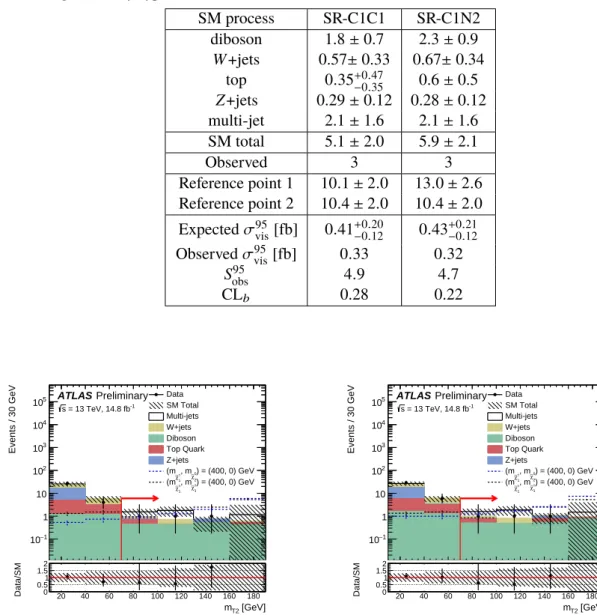
The observed number of events in each signal region and the expected contributions from SM processes are given in Table 6. The contributions of multi-jet and W +jets events were scaled with the normalisation factors obtained from the background-only fit described in Section 8. The multi-jet normalisation in the signal regions has an uncertainty of around 80 %, due to the limited number of observed events in the multi-jet CR-A. The W +jets normalisation is 0.92 ± 0.16. The m T2 distribution is shown in Figure 6 for data, SM expectations, and the SUSY reference points defined in Section 3. In both signal regions, observations and background expectations are found to be compatible within uncertainties.
Using the results of the background-only fit, model-independent upper limits at 95 % confidence level (CL) on the number of non-SM events in the SRs are derived. All limits are calculated using the CL s prescription [98]. Normalising these by the integrated luminosity of the data sample, they can be interpreted as upper limits on the visible non-SM cross section, σ 95
vis , which is defined as the product of acceptance, reconstruction efficiency and production cross section. The accuracy of the limits obtained by the asymptotic formula was tested for all SRs by randomly generating a large number of pseudo-datasets and repeating the fit, and good agreement was found.
10 Interpretation
In the absence of a significant excess over the SM background expectations, the observed and expected numbers of events in the signal regions are used to place model-dependent exclusion limits at 95 % CL using the model-dependent limit fit. SR-C1C1 is used to derive limits for ˜ χ +
1 χ ˜ −
1 production and SR-C1N2 is used to derive limits for the associated production of ˜ χ +
1 χ ˜ −
1 and ˜ χ ±
1 χ ˜ 0
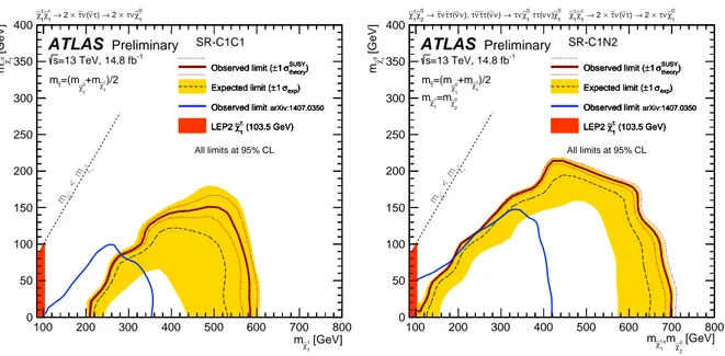
2 . The exclusion limits for the simplified models described in Section 3 are shown in Figure 7. Only ˜ χ +
1 χ ˜ −
1 production is assumed for the left plot, whereas both production processes are considered simultaneously for the right plot. The solid (dashed) lines show the observed (expected) exclusion contours. The band around the expected limit shows the ± 1 σ variations, including all uncertainties except theoretical uncertainties on the signal cross section. The dotted lines around the observed limit indicate the sensitivity to ± 1 σ variations of the theoretical uncertainties on the signal cross section.
Chargino masses up to 580 GeV are excluded for a massless lightest neutralino in the scenario of direct
production of chargino pairs. In the case of associated production of chargino pairs and mass-degenerate
charginos and next-to-lightest neutralinos, chargino masses up to 700 GeV are excluded for a massless
lightest neutralino. These limits improve previous results [34, 35] in the high chargino mass region. The
Table 6: Observed and expected numbers of events in the signal regions for 14.8 fb − 1 . The contributions of multi-jet and W +jets events are scaled with the corresponding normalisation factors. Expected event yields for the SUSY reference points (defined in Section 3) are also given. The shown uncertainties are the sum in quadrature of statistical and systematic uncertainties. The correlation of systematic uncertainties among control regions and among background processes is fully taken into account. The observed and expected 95 % CL upper limits on the visible non-SM cross section ( σ 95
vis ), and the number of signal events ( S 95
obs ) are given. The confidence level observed for the background-only hypothesis, CL b , is also shown.
SM process SR-C1C1 SR-C1N2
diboson 1.8 ± 0.7 2.3 ± 0.9 W +jets 0.57 ± 0.33 0.67 ± 0.34
top 0 . 35 +0 − 0 . . 47 35 0.6 ± 0.5 Z +jets 0.29 ± 0.12 0.28 ± 0.12 multi-jet 2.1 ± 1.6 2.1 ± 1.6 SM total 5.1 ± 2.0 5.9 ± 2.1
Observed 3 3
Reference point 1 10 . 1 ± 2 . 0 13 . 0 ± 2 . 6 Reference point 2 10 . 4 ± 2 . 0 10 . 4 ± 2 . 0 Expected σ 95
vis [fb] 0 . 41 +0 − 0 . . 20 12 0 . 43 +0 − 0 . . 21 12 Observed σ 95
vis [fb] 0 . 33 0 . 32
S 95
obs 4 . 9 4 . 7
CL b 0.28 0.22
[GeV]
m
T220 40 60 80 100 120 140 160 180
Events / 30 GeV
−1
10 1 10 10
210
310
410
5Data SM Total Multi-jets W+jets Diboson Top Quark Z+jets
) = (400, 0) GeV
0 χ∼2
±
, m
χ∼1
(m
) = (400, 0) GeV
± χ∼1
±
, m
χ∼1
(m = 13 TeV, 14.8 fb
-1s
Preliminary ATLAS
[GeV]
m
T220 40 60 80 100 120 140 160 180
Data/SM
0 0.51 1.5 2[GeV]
m
T220 40 60 80 100 120 140 160 180
Events / 30 GeV
−1
10 1 10 10
210
310
410
5Data SM Total Multi-jets W+jets Diboson Top Quark Z+jets
) = (400, 0) GeV
0 χ∼2
±
, m
χ∼1
(m
) = (400, 0) GeV
± χ∼1
±
, m
χ∼1
(m = 13 TeV, 14.8 fb
-1s
Preliminary ATLAS
[GeV]
m
T220 40 60 80 100 120 140 160 180
Data/SM
0 0.51 1.5 2Figure 6: The m T2 distribution before the m T2 requirement is applied for SR-C1C1 (left) and SR-C1N2 (right), where the arrow indicates the position of the cut in the signal region. The stacked histograms show the expected SM backgrounds normalised to 14.8 fb − 1 . The multi-jet contribution is estimated from data using the ABCD method. The contributions of multi-jet and W +jets events are scaled with the corresponding normalisation factors.
The hatched bands represent the sum in quadrature of systematic and statistical uncertainties on the total SM
background. For illustration, the distributions of the SUSY reference points (defined in Section 3) are also shown
as dashed lines. The lower panels show the ratio of data to the total SM background estimate.
[GeV]
± χ∼1
m
100 200 300 400 500 600 700 800
[GeV]
0 1χ∼m
0 50 100 150 200 250 300 350 400
theory) σSUSY
±1 Observed limit (
exp) σ
±1 Expected limit (
arXiv:1407.0350 Observed limit
(103.5 GeV)
± χ∼1 LEP2
)/2
± χ∼1
0
+m
χ∼1 τ∼
=(m m
theory) σSUSY
±1 Observed limit (
exp) σ
±1 Expected limit (
arXiv:1407.0350 Observed limit
(103.5 GeV)
± χ∼1 LEP2
=13 TeV, 14.8 fb
-1s
SR-C1C1
theory) σSUSY
±1 Observed limit (
exp) σ
±1 Expected limit (
arXiv:1407.0350 Observed limit
(103.5 GeV)
± χ∼1 LEP2
1 0χ
∼
< m
1
±χ
m
∼0 χ∼1 ν τ
×
→ 2 τ) ν∼
ν( τ∼
×
→ 2
± χ∼1
± χ∼1
All limits at 95% CL
ATLAS Preliminary
[GeV]
0 χ∼2
,m
± χ∼1
m
100 200 300 400 500 600 700 800
[GeV]
0 1χ∼m
0 50 100 150 200 250 300 350 400
theory) σSUSY
±1 Observed limit (
exp) σ
±1 Expected limit (
arXiv:1407.0350 Observed limit
(103.5 GeV)
± χ∼1 LEP2
)/2
± χ∼1
0
+m
χ∼1 τ∼
=(m m
0 χ∼2
=m
± χ∼1
m
theory) σSUSY
±1 Observed limit (
exp) σ
±1 Expected limit (
arXiv:1407.0350 Observed limit
(103.5 GeV)
± χ∼1 LEP2
=13 TeV, 14.8 fb
-1s
SR-C1N2
theory) σSUSY
±1 Observed limit (
exp) σ
±1 Expected limit (
arXiv:1407.0350 Observed limit
(103.5 GeV)
± χ∼1 LEP2
1 0χ
∼
< m
1
±χ
m
∼0 χ∼1 ν τ
×
→ 2 τ) ν∼
ν( τ∼
×
→ 2
± χ∼1
± χ∼1 0 χ∼1 ν) ν τ( 0τ χ∼1 ν τ
→ ν) ν∼
τ( τ∼
ν∼
τ ν), ν∼
τ( τ∼
ν τ∼
0→ χ∼2
± χ∼1