s = 13TeVproton–protoncollisiondata √ SearchfornewphenomenainaleptonplushighjetmultiplicityfinalstatewiththeATLASexperimentusing ATLASCONFNote

ATLAS-CONF-2017-013 31March2017

ATLAS CONF Note

ATLAS-CONF-2017-013

Search for new phenomena in a lepton plus high jet multiplicity final state with the ATLAS experiment

using √

s = 13 TeV proton–proton collision data

The ATLAS Collaboration

17th March 2017

A search for new phenomena in final states characterized by high jet multiplicity, an isolated lepton (electron or muon) and either zero or at least three b -tagged jets is presented. The search uses 36.1 fb

of

√ s = 13 TeV proton–proton collision data collected by the ATLAS experiment at the Large Hadron Collider in 2015 and 2016. The dominant sources of back- ground are estimated using parameterized extrapolations, based on observables at medium jet multiplicity, to predict the b -tagged jet distribution at the higher jet multiplicities used in the search. No significant excess over the Standard Model expectation is observed and 95%

confidence level limits are extracted constraining four simplified models of R -Parity violating supersymmetry that feature either gluino or top squark pair-production. The exclusion limits reach up to 2.1 TeV in gluino mass and up to 1.2 TeV in top squark mass in the models considered. In addition, an upper limit is set on the cross-section for Standard Model t tt¯ ¯ t production of 60 fb (6.5 × the Standard Model prediction) at 95% confidence level. Finally, model-independent limits are set on the contribution of new phenomena to the signal region yields.

© 2017 CERN for the benefit of the ATLAS Collaboration.

Reproduction of this article or parts of it is allowed as specified in the CC-BY-4.0 license.

1 Introduction

The ATLAS experiment at the Large Hadron Collider has carried out a large number of searches for beyond the Standard Model (BSM) physics covering a broad range of different final-state particles and kinematics. However, one gap in the search coverage, as pointed out in Refs. [1, 2], is in final states with one or more leptons, many jets and no-or-little missing transverse momentum (the magnitude of which is denoted as E

T

). Such a search is presented in this article, considering final states with an isolated lepton (electron or muon), at least eight to twelve jets (depending on the jet transverse momentum threshold) and either zero or many b-tagged jets and with no requirement on E

T

.

This search has potential sensitivity to a large number of BSM physics models. In this article, model- independent limits on the possible contribution of BSM physics to several single-bin signal regions are presented. In addition, four R -parity violating (RPV) supersymmetric (SUSY [3–8]) benchmark models are used to interpret the results. In this case a multi-bin fit to the two-dimensional jet-multiplicity, and b -tagged jet multiplicity space is used to constrain the models. The dominant Standard Model (SM) background arises from top-quark pair production and W +jets production. The precise theoretical modelling of these backgrounds at high jet multiplicity suffers from large uncertainties, hence they are estimated from the data by extrapolating the b -tagged jet multiplicity distribution extracted at moderate jet multiplicities to the high jet multiplicities of the search region.

The result is also used to search for SM four top-quark production. Previous searches for four top-quark production have been carried out by the ATLAS [9] and CMS [10] Collaborations.

This article is organized as follows: Sections 2 and 3 briefly describe the ATLAS detector and the data and simulated event samples used. Section 4 details the object selection, Section 5 the analysis strategy, Section 6 the background estimation, Section 7 the background validation and Section 8 the systematic uncertainties. The results are presented in Section 9, before concluding in Section 10.

2 The ATLAS detector

The ATLAS detector [11] is a multi-purpose detector with a forward-backward symmetric cylindrical geometry and nearly 4 π coverage in solid angle.1 The inner tracking detector (ID) consists of silicon pixel and microstrip detectors covering the pseudorapidity region | η | < 2.5, surrounded by a transition radiation tracker which improves electron identification over the region | η | < 2.0. The innermost pixel layer, the insertable B-layer [12], was added between Run 1 and Run 2 of the LHC, at a radius of 33 mm around a new, narrower and thinner, beam pipe. The ID is surrounded by a thin superconducting solenoid providing an axial 2 T magnetic field and by a fine-granularity lead/liquid-argon (LAr) electromagnetic calorimeter covering | η | < 3.2. A steel/scintillator-tile calorimeter provides hadronic calorimetry in the central pseudorapidity range (| η | < 1.7). The endcap and forward regions (1.5 < | η | < 4.9) of the hadronic calorimeter are made of LAr active layers with either copper or tungsten as the absorber material. The

1ATLAS uses a right-handed coordinate system with its origin at the nominal interaction point in the centre of the detector.

The positivex-axis is defined by the direction from the interaction point to the centre of the LHC ring, with the positive y-axis pointing upwards, while the beam direction defines thez-axis. Cylindrical coordinates (r,φ) are used in the transverse plane, φ being the azimuthal angle around the z-axis. The pseudorapidityη is defined in terms of the polar angleθby η =−ln tan(θ/2). The transverse momentump_Tis defined in thex–yplane unless stated otherwise. Rapidity is defined asy=0.5 ln

(E+p_z)/(E−p_z)

whereEdenotes the energy andp_zis the component of the momentum along the beam direction.

muon spectrometer with an air-core toroid magnet system surrounds the calorimeters. Three layers of high-precision tracking chambers provide coverage in the range | η | < 2.7, while dedicated chambers allow triggering in the region | η | < 2.4.

The ATLAS trigger system [13, 14] consists of two levels; the first level is a hardware-based system, while the second is a software-based system called the High-Level Trigger.

3 Data and simulated samples

3.1 Data sample

After applying beam, detector and data-quality criteria, the data sample analyzed comprises of 36.1 fb

of

√ s = 13 TeV proton–proton ( pp ) collision data (3.2 fb

collected in 2015 and 32.9 fb

collected in 2016) with a minimum pp bunch spacing of 25 ns. In this dataset, the mean number of pp interactions per proton-bunch crossing (pile-up) is hµi = 23.7. The luminosity and its uncertainty of ± 3 . 2% are derived following a methodology similar to that detailed in Ref. [15] from a preliminary calibration of the luminosity scale using a pair of x – y beam separation scans performed in August 2015 and June 2016.

Events are recorded online using a single electron or muon trigger with thresholds that give constant efficiency of ≈ 90% ( ≈ 80%) for electrons (muons) for the event selection used. For the determination of the multi-jet background, lepton triggers with less stringent lepton isolation requirements are used as discussed in Section 6. Single photon and multi-jet triggers are also employed to select data samples used in the validation of the background estimation technique.

3.2 Simulated event samples

Samples of Monte Carlo (MC) simulated events are used to model the signal and to validate the background estimation procedure for the dominant background contributions. In addition, simulated events are used to model the sub-dominant background processes. The response of the detector to particles is modelled with a full ATLAS detector simulation [16] based on Geant4 [17], or with a fast simulation based on a parameterization of the response of the ATLAS electromagnetic and hadronic calorimeters [18]

and on Geant4 elsewhere. All simulated events are overlaid with pile-up collisions simulated with the soft QCD processes of Pythia 8.186 [19] using the A2 set of tunable parameters (tune) [20] and the MSTW2008LO [21] parton distribution function (PDF) set. The simulated events are reconstructed in the same way as the data, and are reweighted so that the distribution of the expected number of collisions per bunch crossing matches the one in the data.

For all MC samples used, except those produced by the Sherpa generator, the EvtGen v1.2.0 program [22]

is used to model the properties of bottom and charm hadron decays.

3.2.1 Simulated signal events

Simulated signal events from four SUSY benchmark models are used to guide the analysis selections and

to estimate the expected signal yields for different signal mass hypotheses used to interpret the analysis

results. In all models, the RPV couplings and the SUSY particle masses are chosen to ensure prompt

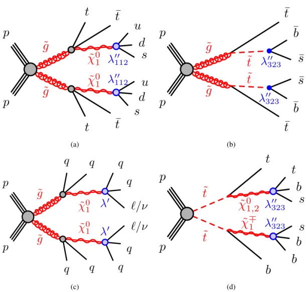
decays of the SUSY particles. Diagrams of the first three benchmark simplified models which involve gluino pair production are shown in Figure 1 (a), (b), and (c). In the first model, each gluino decays via a virtual top squark to two top quarks and the lightest neutralino ( ˜ χ

1

), with the ˜ χ

1

decaying to three light quarks ( ˜ χ

1

→ uds ) via the RPV coupling λ

112

. For this model ˜ χ

1

masses below 10 GeV are not considered to avoid the effect of the limited phase-space in the ˜ χ

1

decay. In the second model, each gluino decays to a top quark and a top squark, with the top squark decaying to an s - and a b - quark via a non-zero λ

323

RPV coupling.2 The third model involves the gluino decaying to two light quarks ( q ≡ (u, d, s, c)) and the ˜ χ

1

, which then decays to two light quarks and a charged lepton or a neutrino ( ˜ χ

1

→ qq`/ν ) via a λ

RPV coupling, where each RPV decay can produce any of the four first and second generation leptons ( e

, µ

, ν

, ν

) with equal probability. For this model ˜ χ

1

masses below 50 GeV are not considered.

The fourth scenario considered involves right-handed top squark pair production with the top squark decaying to a bino or higgsino lightest supersymmetric particle (LSP). The LSP decays through the non- zero RPV coupling λ

323

≈ O (10

− 10

), with the value chosen to ensure prompt decays for the particle masses considered3 and to avoid more complex patterns of RPV decays that are not considered here.

Figure 1 d) shows the production and possible decays considered. The different decay modes depend on the nature of the LSP and have a small dependence on the top squark mass, with the top squark decaying as:

t ˜ → t χ ˜

1

for a bino-like LSP and as ˜ t → t χ ˜

2

( ≈ 25%), ˜ t → t χ ˜

1

( ≈ 25%), ˜ t → b χ ˜

1

( ≈ 50%) for higgsino-like LSPs. With the chosen model parameters, the electroweakinos decay as ˜ χ

1/2

→ tbs or ˜ χ

1

→ bbs . The search results are interpreted in this model, with the assumption of either a pure higgsino ( ˜ H ) or pure bino ( ˜ B ) LSP. In the case of a wino LSP the search has no sensitivity as the top squark decays directly as t ˜ → bs with no leptons produced in the final state. For this case a dedicated ATLAS search [25] excludes top squark masses up to 315 GeV.

Event samples for the first signal model ( ˜ g → t¯ t χ ˜

1

→ t¯ tuds ) are produced using the Herwig++ 2.7.1 [26]

generator with the cteq6l1 [27] PDF set, and using the UEEE5 tune [28]. For the other three models, the MG5_aMC@NLO v2.3.3 [29] generator interfaced to Pythia 8.210 is used. For these cases, signal events are produced with either one ( ˜ g → t ¯ t ˜ → tbs ¯ model) or two ( ˜ g → q q ¯ χ ˜

1

→ q q`/ν ¯ qq and ˜ t → t H/ ˜ B ˜ models) additional partons in the matrix element and using the A14 [30] tune. The parton luminosities are provided by the NNPDF23LO [31] PDF set.

Signal cross-sections are calculated to next-to-leading order in the strong coupling constant, adding the resummation of soft-gluon emission at next-to-leading-logarithmic accuracy (NLO+NLL) [32–36]. The nominal cross-section and the uncertainty are taken from an envelope of cross-section predictions using different PDF sets and factorisation and renormalisation scales, as described in Ref. [37].

The result is also used to search for SM four-top-quark production. In this case, the t tt¯ ¯ t sample is generated with the MG5_aMC@NLO v2.2.2 generator interfaced to Pythia 8.186 using the NNPDF23LO PDF set and the A14 tune.

3.2.2 Simulated background events

The dominant backgrounds from top-quark pair production and W /Z +jets production are estimated from the data as described in Section 6, whereas the expected yields for minor backgrounds are taken from

2The same final state can be produced by requiring a non-zeroλ⁰⁰

313 RPV coupling, however the minimal flavour violation hypothesis [23] favours a largeλ⁰⁰

323coupling [24].

3LSP masses below 200 GeV are not considered as in this case non-prompt RPV decays can occur.

˜ g

˜ g

˜ χ ⁰ ₁

˜ χ ⁰ ₁ p

p

t t ¯

λ

u

d s

t t ¯ λ

s d

u

(a)

˜ g

˜ g

t ˜ t ˜ p

p

¯ t

λ

s ¯

¯ b

¯ t λ

¯ s

¯ b

(b)

˜ g

˜ g

˜ χ ⁰ ₁

˜ χ ⁰ ₁ p

p

q q

λ ^′ q q

ℓ/ν

q q

λ ^′ q

q ℓ/ν

(c)

˜ t

˜ t

˜ χ ⁰ _1,2

˜ χ ^∓ ₁ p

p

t

λ

t b s

b

λ

b b

s

(d)

Figure 1: Diagrams of the four simplified signal benchmark models considered. The first three models involve pair production of gluinos with each gluino decaying as (a) ˜g → t¯tχ˜⁰

1 →ttuds¯ , (b) ˜g →t¯t˜→ t¯b¯s¯, (c) ˜g → qqχ˜⁰

1 → qqqq`/ν. The fourth model (d) involves pair production of top squarks with the decay ˜t →tχ˜⁰

1/2or ˜t →bχ˜^±

1 and with the LSP decays ˜χ⁰_1/2 →tbsor ˜χ^±

1 → bbs; the specific decay depends on the nature of the LSP. In all signal scenarios, anti-squarks decay into the charge-conjugate final states of those indicated for the corresponding squarks, and each gluino decays with equal probabilities into the given final state or its charge conjugate.

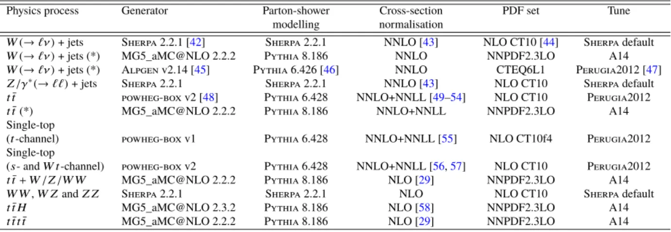
Monte Carlo simulation. In addition, the background estimation procedure is validated with simulated events, and some of the systematic uncertainties are estimated using simulated samples. The samples used are shown in Table 1 and more details on the generator configurations can be found in Refs. [38–41].

4 Object reconstruction

For a given event, primary vertex candidates are required to be consistent with the luminous region and to have at least two associated tracks with p

> 400 MeV. The vertex with the largest P

p

T

of the associated

tracks is chosen as the primary vertex of the event.

Physics process Generator Parton-shower Cross-section PDF set Tune modelling normalisation

W(→`ν)+ jets Sherpa 2.2.1 [42] Sherpa 2.2.1 NNLO [43] NLO CT10 [44] Sherpa default

W(→`ν)+ jets (*) MG5_aMC@NLO 2.2.2 Pythia 8.186 NNLO NNPDF2.3LO A14

W(→`ν)+ jets (*) Alpgen v2.14 [45] Pythia 6.426 [46] NNLO CTEQ6L1 Perugia2012 [47]

Z/γ^∗(→``)+ jets Sherpa 2.2.1 Sherpa 2.2.1 NNLO [43] NLO CT10 Sherpa default tt¯ powheg-box v2 [48] Pythia 6.428 NNLO+NNLL [49–54] NLO CT10 Perugia2012

tt¯(*) MG5_aMC@NLO 2.2.2 Pythia 8.186 NNLO+NNLL NNPDF2.3LO A14

Single-top

(t-channel) powheg-box v1 Pythia 6.428 NNLO+NNLL [55] NLO CT10f4 Perugia2012 Single-top

(s- andW t-channel) powheg-box v2 Pythia 6.428 NNLO+NNLL [56,57] NLO CT10 Perugia2012

tt¯+W/Z/W W MG5_aMC@NLO 2.2.2 Pythia 8.186 NLO [29] NNPDF2.3LO A14

W W,W ZandZ Z Sherpa 2.2.1 Sherpa 2.2.1 NLO NLO CT10 Sherpa default

tt H¯ MG5_aMC@NLO 2.3.2 Pythia 8.186 NLO [58] NNPDF2.3LO A14

tt t¯ t¯ MG5_aMC@NLO 2.2.2 Pythia 8.186 NLO [29] NNPDF2.3LO A14

Table 1: Simulated background event samples: the corresponding generator, parton-shower modelling, cross-section normalisation, PDF set and underlying-event tune are shown. The samples marked with (*) are alternative samples used to validate the background estimation method.

Jet candidates are reconstructed using the anti- k

jet clustering algorithm [59, 60] with a radius parameter of 0 . 4 starting from energy clusters of calorimeter cells [61]. The jets are corrected for energy deposits from pile-up collisions using the method suggested in Ref. [62] and calibrated with ATLAS data in Ref. [63]: a contribution equal to the product of the jet area with the median energy density of the event is subtracted from the jet energy. Further corrections derived from MC simulation and data are used to calibrate on average the energies of jets to the scale of their constituent particles [64]. In the search, three jet p

thresholds are used, p

> 40 GeV, p

> 60 GeV, and p

> 80 GeV, with all jets required to be within |η | < 2 . 4. To minimize the contribution from jets arising from pile-up interactions, the selected jets must satisfy a loose jet vertex tagger (JVT) requirement [65], where JVT is a quantity that uses tracking and primary vertex information to determine if a given jet originates from the primary vertex.

The chosen working point has an efficiency of 94% at a jet p

of 40 GeV and is nearly fully efficient above 60 GeV for jets originating from the hard parton–parton scatter. This selection reduces the number of jets originating from, or heavily contaminated by, pile-up interactions, to a negligible level. Events with jet candidates originating from detector noise and non-collision background are rejected if the jet candidates fail to satisfy the ‘LooseBad’ quality criteria, described in Ref. [66]. The coverage of the calorimeter and the jet reconstruction techniques allow high jet multiplicity final states to be efficiently reconstructed. For example, 12 jets only take up about one fifth of the available solid angle.

Jets containing a b -hadron ( b -jets) are identified by a multivariate algorithm using information about the impact parameters of ID tracks matched to the jet, the presence of displaced secondary vertices, and the reconstructed flight paths of b - and c - hadrons inside the jet [67]. The operating point used corresponds to an efficiency of 78% in simulated t¯ t events, along with a rejection factor of 114 for jets induced by gluons or light-quarks and of 7.6 for charm jets [68], and is configured to give a constant b -tagging efficiency as a function of jet p

.

Since there is no requirement on E

T

or the transverse mass4, the search is particularly sensitive to fake or non-prompt leptons in multi-jet events. In order to suppress this background to an acceptable level, stringent lepton identification and isolation requirements are used.

4The transverse mass between the lepton and theE^missis defined as:m² =2p_T<sup>`</sup>E<sup>miss</sup>(1−cos(∆φ(`,E^miss)))

Muon candidates are formed by combining information from the muon spectrometer and the ID and must satisfy the ’Medium’ quality criteria as described in Ref. [69]. They are required to have p

> 30 GeV and |η| < 2 . 4. Furthermore, they must satisfy requirements on the significance of the transverse impact parameter with respect to the primary vertex, |d

0

|/σ( d

0

) < 3, the longitudinal impact parameter with respect to the primary vertex, | z

0

sin(θ ) | < 0.5 mm, and the ‘Gradient’ isolation requirements described in Ref. [69] relying on a set of η - and p

-dependent criteria based on tracking and calorimeter related variables.

Electron candidates are reconstructed from an isolated electromagnetic calorimeter energy deposit matched to an ID track and are required to have p

> 30 GeV, |η| < 2 . 47, and to satisfy the ‘Tight’ likelihood-based identification criteria described in Ref. [70]. Electron candidates that fall in the transition region between the barrel and end-cap calorimeter (with 1 . 37 < |η| < 1 . 52) are rejected. They are also required to have

| d

0

|/σ (d

0

) < 5, |z

0

sin (θ) | < 0.5 mm, and to satisfy similar isolation requirements to those applied to muon candidates.

An overlap removal procedure is carried out to resolve ambiguities between candidate jets (with p

>

20 GeV) and baseline leptons5 as follows: first, any non- b -tagged jet candidate6 lying within an angular distance ∆R ≡ p

( ∆ y)

+ ( ∆φ)

= 0 . 2 of a baseline electron is discarded. Furthermore, non- b -tagged jets within ∆R = 0 . 4 from baseline muons are removed if the number of tracks associated with the jet is less than three or the ratio of the muon to jet p

is greater than 0.5. Finally, any baseline lepton candidate remaining within a distance ∆R = 0 . 4 of any surviving jet candidate is discarded.

Corrections derived from data control samples are applied to account for differences between data and simulation for the lepton trigger, reconstruction, identification and isolation efficiencies, the lepton mo- mentum/energy scale and resolution [69, 71], and for the efficiency and mis-tag rate of the b -tagging algorithm [67].

5 Event selection and analysis strategy

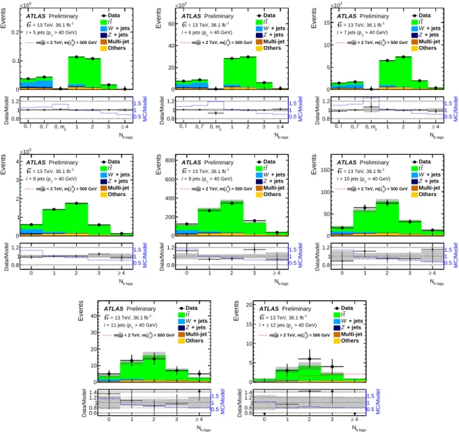
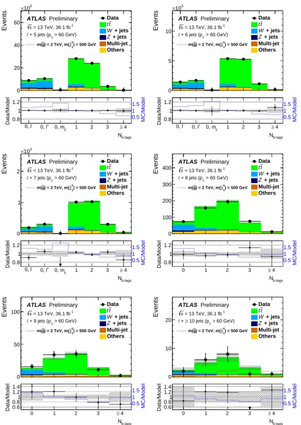
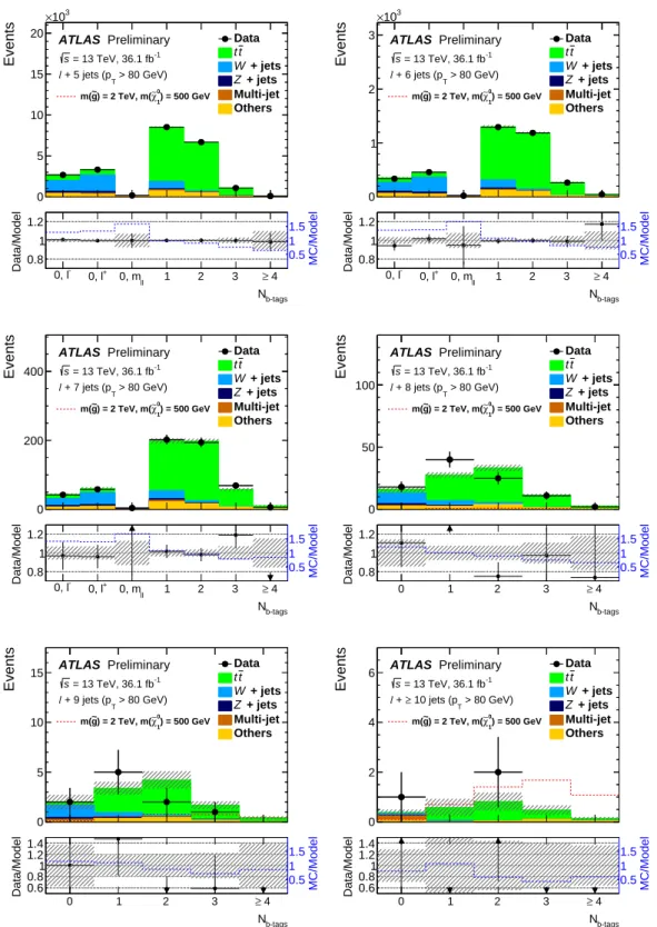
Events are selected online using a single electron or muon trigger. For the analysis selection, at least one electron or muon, matched to the trigger lepton, is required in the event. The analysis is carried out with three sets of jet p

thresholds to provide sensitivity to a broad range of possible signals. These thresholds are applied to all jets in the event and are p

> 40 GeV, p

> 60 GeV and p

> 80 GeV. The jet multiplicity is binned from a minimum of five jets to a maximum number that depends on the p

threshold. The last bin is inclusive, so that it also includes all events with more jets than the bin number. This bin corresponds to 12 or more jets for the 40 GeV requirement, and 10 or more jets for the 60 GeV and 80 GeV thresholds.

There are five bins in the b -tagged jet multiplicity (exclusive bins from zero to three with an additional inclusive four-or-more bin). In this article, the notation N

is used to denote the number of events predicted by the background fit model, with j jets and b b -tagged jets for a given process, e.g. N

for t t ¯ +jets events. The number of events summed over all b -tag multiplicity bins for a given number of jets is denoted by N

, and is also referred to as a jet-slice.

5Baseline leptons are reconstructed as described above, but with a looserp_Trequirement (p_T>10 GeV), no isolation or impact parameter requirements, and, in the case of electrons, the ’Loose’ lepton identification criteria [70].

6In this case, ab-tagging working point corresponding to an efficiency of identifyingb-jets in a simulatedt¯tsample of 85% is used.

For probing a specific BSM model, all of these bins in data are simultaneously fit to constrain the model, in what is labeled a model-dependent fit. In the search for an unknown BSM signal, dedicated signal regions (SRs) are defined which could be populated by a possible signal, and where the SM contribution is expected to be small. The expected background in these SRs is estimated from a fit for which some of the bins can be excluded to limit the effect of signal contamination biasing the background estimate; this setup is labeled a model-independent fit. More details on the SR definitions are given in Section 7.

An example of the expected background contributions from MC simulation for the different b -tag bins, with a selection of at least ten jets, can be seen in Figure 2. This figure shows that the background in the zero b -tag bin is dominated by W +jets and t t ¯ +jets, whereas in the other b -tag bins it is completely dominated by t¯ t +jets. The contribution from other processes is very small in all bins.

b-tags

N

0 1 2 3 ≥ 4

Events

0 50 100

150 t t

+ jets W

+ jets Z

Multi-jet Others

= 13 TeV, 36.1 fb-1

s

l > 40 GeV)

10 jets (pT

≥ +

ATLAS Simulation Preliminary

Figure 2: The expected background from MC simulation in the differentb-tag bins, with a selection of at least ten jets (with a 40 GeV jetp_Tthreshold).

The estimation of the dominant background processes of t¯ t +jets and W/Z +jets production is carried out using a combined fit to the jet and b -tagged jet multiplicity bins described above. For these backgrounds the normalization per jet slice is derived using parameterized extrapolations from lower jet multiplicities.

The b -tag multiplicity shape per jet slice is taken from simulation for the W/ Z +jets background, whereas

for the t¯ t +jets background it is predicted from the data using a parameterized extrapolation based on

observables at medium jet multiplicities. A separate likelihood fit is carried out for each jet p

threshold,

with the fit parameters of the background model determined separately in each fit. The assumptions used in

the parameterization are validated using data and MC simulation. Furthermore, for the model-independent

results, the background determination assumes that there is no significant signal contribution to events

with five, six or seven jets. Signal processes with final states that the search is targeting generally have

negligible leakage into these jet slices, as for example is the case for the benchmark models considered.

6 Background estimation

6.1 W /Z +jets

A partially data-driven approach is used to estimate the W /Z +jets background. Since the W/Z +jets background predominantely has no b -jets, the shape of the b -tag multiplicity spectra are taken from simulated events, whereas the normalization in each jet slice is derived from the data. The estimate of the normalization relies on assuming a functional form to describe the evolution of the number of W/Z +jets events as a function of the jet multiplicity, r ( j) ≡ N

/N

.

Above a certain number of jets, r ( j) can be assumed to be a constant r , implying a fixed probability of additional jet radiation, referred to as “staircase scaling” [72–75]. This behaviour has been observed by the ATLAS [76, 77] and CMS [78] Collaborations. For lower jet multiplicities, a different scaling is expected with r ( j) = k /( j + 1) where k is a constant, referred to as “Poisson scaling” [75].7

For the kinematic phase-space relevant for this search, a combination of the two scalings has been found to describe the data in dedicated validation regions (described later in this section), as well as in high equivalent luminosity Monte Carlo simulations of W/Z +jets events. This combined scaling is parameterized as

r ( j) = c

+ c

/( j + 1) (1)

where c

and c

are constants that are extracted from the data. Studies demonstrate that the flexibility of this parameterization is also able to absorb reconstruction effects related to the decrease of the efficiency for reconstructing events with increasing jet multiplicity mainly due to the lepton-jet overlap and the lepton isolation requirements.

The number of W +jets or Z +jets events with different jet and b -jet multiplicities, N

, is then parameterized as follows:

N

= MC

MC

· N

·

j⁰=j−1

Y

j⁰=5

r ( j

), (2)

where MC

and MC

are the predicted numbers of W/Z + j jets events with b b -tags and inclusive in b -tags, respectively, both taken from MC simulation, and N

is the absolute normalization in five-jet events. The term N

· Q

j⁰=5

r ( j

) gives the number of b -tag inclusive events in jet slice j , and the ratio MC

/ MC

is the fraction of b b -tagged events in this jet slice. The four parameters N

, N

, c

, c

are left floating in the fit and are therefore extracted from the data along with the other background contributions.

Due to different b -tagged jet multiplicity spectra in W +jets and Z +jets events, the b -tag distribution is modeled separately for the two processes. The normalization and scaling parameters N

, c

, c

are determined using control regions with five, six or seven jets and zero b -tags. For the Z +jets background determination, the control regions are defined selecting events with two oppositely charged same flavour leptons fulfilling an invariant-mass requirement around the Z -boson mass (81 ≤ m

≤ 101 GeV), as well as the requirement of exactly five, exactly six or exactly seven jets, and zero b -tags. The determination of

7The transition between these scaling behaviours depends on the jet kinematic selections.

the W +jets background relies on control regions containing the remaining events with exactly five, six or seven jets, and zero b -tags, which, for each jet multiplicity, is split by the electric charge of the highest- p

lepton. The expected charge asymmetry in W +jets events is taken from MC simulation separately for five-jet, six-jet and seven-jet events and used to constrain the W +jets normalization from the data using these control regions. Although all parameters are determined in a global likelihood fit, the dominant constraining power on the absolute normalization comes from the five-jet control regions, and the dominant constraints on the c

and c

parameters originate from the combination of the five-jet, six-jet and seven-jet control regions. The contamination of t t ¯ events in the Z +jets two lepton control regions is negligible, whereas in the control regions used to estimate the W +jets normalization it is significant and is discussed in Section 6.2. Once the W +jets and Z +jets backgrounds are normalized, they are extrapolated to higher jet multiplicities using the same common scaling function r ( j). While independent scalings could be used, tests in data show no significant difference and therefore a common function is used.

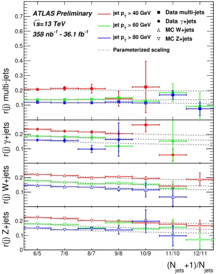
The jet scaling assumption is validated in data using γ +jets and multi-jet events, and also simulated W +jets and Z +jets samples are found to be consistent with this assumption. The γ +jets events are selected using a photon trigger, and an isolated photon [79] with p

> 145 GeV is required in the event selection, whereas the multi-jet events are selected using prescaled and unprescaled multi-jet triggers. In both cases, selections are applied to ensure these control regions probe a kinematic phase-space region similar to the one relevant for the analysis.

Figure 3 shows the r ( j) ratio for various processes used to validate the jet scaling parameterization. Each panel shows the ratio for data or MC with the fitted parameterization overlaid as a line. In the case of pure

“staircase scaling”, the shown ratio would be a constant.

6.2 t t+jets ¯

A data-driven model is used to estimate the number of events from t¯ t +jets production in a given jet and b -tag multiplicity bin. The basic concept of this model is based on the extraction of an initial template of the b -tag multiplicity spectrum in events with five jets and the parameterization of the evolution of this template to higher jet multiplicities. The absolute normalization for each jet-multiplicity slice is constrained in the fit as discussed later in this section. Figure 4 shows the b -tag multiplicity distributions in t¯ t +jets MC simulation, for five, eight and ten jet events, demonstrating how the distributions evolve as the number of jets increases. The background estimation parameterizes this effect and extracts the parameters describing the evolution from a fit to the data.

The extrapolation of the b -tag multiplicity spectrum to higher jet multiplicities starts from the assumption that the difference in the b -tag multiplicity spectrum in events with j and j + 1 jets arises mainly from the production of additional jets, and can be described by a fixed probability that the additional jet is b -tagged. Given the small mistag rate, this probability is dominated by the probability that the additional jet is a heavy-flavour jet which is b -tagged. In order to account for acceptance effects due to the different kinematics in events with high jet multiplicity, the probability of further b -tagged jets entering into acceptance is also taken into account. The extrapolation over one additional jet can be parameterized as:

N

= N

· f

f

= f

· x

+ f

· x

+ f

· x

(3)

+1)/N

(N

6/5 7/6 8/7 9/8 10/9 11/10 12/11

r(j) Z+jets

0 0.1 0.2

6/5 7/6 8/7 9/8 10/9 11/10 12/11

r(j) W+jets

0.1 0.2

6/5 7/6 8/7 9/8 10/9 11/10 12/11

+jets γ r(j)

0.2

r(j) multi-jets

0.2 0.3 0.4 0.5 0.6

0.7 > 40 GeV

jet pT

> 60 GeV jet pT

> 80 GeV jet pT

Parameterized scaling

Data multi-jets +jets Data γ MC W+jets MC Z+jets ATLAS Preliminary

=13 TeV s

- 36.1 fb-1

358 nb-1

Figure 3: The ratio of the number of events with (j+1) to j jets for various processes used to validate the jet scaling-parameterization. Each panel shows the ratio for data or MC with the fitted parameterization overlaid as a line. In the case of pure “staircase scaling”, the shown ratio would be a constant. For the multi-jet data points the 40 GeV jetp_Tselection uses a prescaled trigger corresponding to a luminosity of 358 nb⁻¹, all other selections used unprescaled triggers corresponding to the full dataset.

where N

is the number of t t ¯ +jets events with j jets and f

is the fraction of t¯ t events with j jets of which b are b -tagged. The parameters x

describe the probability of one additional jet to be either not b -tagged ( x

), b -tagged ( x

), or b -tagged and leading to a second b -tagged jet to move into the fiducial acceptance ( x

). The latter is dominated by cases where the extra jet is a b -jet and it influences the kinematics of the event such that an additional b -jet, that was below the jet p

threshold, enters into the acceptance. Given that the x

parameters describe probabilities, the sum P

i

x

is normalized to unity. Subsequent application of this parameterization produces a b -tag template for arbitrarily high jet multiplicities.

Studies based on MC simulated events corresponding to very large equivalent luminosities as well as

studies using fully efficient truth-level b -tagging indicate the necessity to add a fit parameter that allows

for correlated production of two b -tagged jets as may be expected with b -jet production from gluon

b-tags

N

0 1 2 3 ≥ 4

normalized to unity

0 0.2 0.4

0.6 5 jets

8 jets 10 jets

MC t = 13 TeV, t s

> 40 GeV jet pT

ATLAS Simulation Preliminary

Figure 4: The normalizedb-tag distribution fromtt¯+jets MC simulation events for five, eight and ten jet events (with a 40 GeVp_Tthreshold).

splitting. This is implemented by changing the evolution described in Equation 3 such that any term with x

· x

is replaced by x

· x

· ρ

, where ρ

describes the correlated production of two b -tagged jets.

The initial b -tag multiplicity template is extracted from data events with five jets after subtracting all other background processes, and is denoted as f

and scaled by the absolute normalization N

5

in order to obtain the model in the five-jet bin:

N

5,b

= N

5

· f

(4)

where the sum of f

over the five b -tag bins is normalized to unity.

The model described above is based on the assumption that any change of the b -tag multiplicity spectrum is due to additional jet radiation with a certain probability to lead to b -tagged jets. There is, however, also a small increase in the acceptance for b -jets produced in the decay of the t¯ t system when increasing the jet multiplicity due to the higher jet momentum on average. The effect amounts to up to 5% in the one and two b -tag bins for high jet multiplicities, and is taken into account using a correction to the initial template extracted from simulated t¯ t events.

As for the W/Z +jets background, the normalization of the t t ¯ background in each jet slice is constrained using a scaling behaviour similar to that in Equation 1. The parameterization is slightly modified to:

N

/N

≡ r

( j) = c

0

+ c

1

/( j + c

2

) (5)

where the three parameters c

0

, c

1

and c

2

are extracted from a fit to the data. Here j is the number of additional jets not originating from the t¯ t decay, and the denominator ( j + 1 ) in Equation 1 is replaced by ( j + c

2

) to take into account the ambiguity in the counting of additional jets due to

acceptance effects on the t¯ t decay products. The scaling behaviour is tested in t¯ t +jets MC simulated

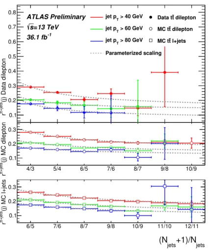
samples (both the nominal sample and the alternative sample described in Table 1), and also in data with a dileptonic t¯ t +jets control sample. This sample is selected by requiring an electron and muon candidate in the event, with at least three jets of which at least one is b -tagged, and the small background in this sample is subtracted using the MC simulation expectations. In this control region the scaling behaviour can be tested for up to eight jets, but this corresponds to ten jets for a semileptonic t¯ t +jets sample (which is the dominant component of the t¯ t +jets background). Figure 5 presents the comparison of the scaling behaviour in data and MC compared to a fit of the parameterization used and shows that the assumed function describes the data and MC well for the jet-multiplicity range relevant for this search.

Since the last jet-multiplicity bin used in the analysis is inclusive in the number of jets, the model is used to predict this by iterating to much higher jet multiplicities and summing the contribution for each jet multiplicity above the maximum used in the analysis, therefore giving the correct inclusive yield in this bin.

The zero b -tag component of the initial t t ¯ template, which is extracted from events with five jets, exhibits an anti-correlation with the absolute W +jets normalization which is extracted in the same bin. The control regions separated in leading-lepton charge, detailed in Section 6.1, provide a handle to extract the absolute W +jets normalization. The remaining anti-correlation does not affect the total background estimate. For these control regions the t¯ t +jets process is assumed to be charge symmetric and the model is simply split into two halves for these bins.

6.3 Multi-jet events

The contribution from multi-jet production with a fake or non-prompt (FNP) lepton (such as hadrons mis-identified as leptons, leptons originating from the decay of heavy-flavour hadrons, and electrons from photon conversions), constitutes a minor but non-negligible background, especially in the lower jet-multiplicity slices. It is estimated from the data with a matrix method similar to that described in Ref. [80]. In this method, two types of lepton identification criteria are defined: “tight”, corresponding to the default lepton criteria described in Section 4, and “loose”, corresponding to baseline leptons after overlap removal. The matrix method relates the number of events containing prompt or FNP leptons to the number of observed events with tight or loose-not-tight leptons using the probability for loose-prompt or loose-FNP leptons to satisfy the tight criteria. The probability for loose-prompt leptons to satisfy the tight selection criteria is obtained using a Z → `` data sample and is modelled as a function of the lepton p

. The probability for loose FNP leptons to satisfy the tight selection criteria is determined from a data control region enriched in non-prompt leptons requiring a loose lepton, multiple jets, low E

T

[81, 82] and low transverse mass. The efficiencies are measured as a function of p

after subtracting the contribution from prompt lepton processes and are assumed to be independent of the jet multiplicity.8

6.4 Small backgrounds

The small background contribution from diboson production, single-top production, t¯ t production in association with a vector/Higgs boson (labeled t tV ¯ /H ) and SM four-top-quark production are estimated using MC simulated event samples. In all but the highest jet-multiplicity slices considered, the sum of

8To minimise the dependence on the number of jets, the event selection considers only the leading-p_Tbaseline lepton when checking the more stringent identification and isolation criteria of the “tight” lepton definitions.

+1)/N

(N

6/5 7/6 8/7 9/8 10/9 11/10 12/11

(j) MC l+jets+jetstt r 0.1 0.2 0.3

4/3 5/4 6/5 7/6 8/7 9/8 10/9

(j) MC dilepton+jetstt r 0.1 0.2 0.3 (j) Data dilepton +jetstt r _0.1 0.2 0.3 0.4 0.5 0.6 0.7

0.8 > 40 GeV

jet pT

> 60 GeV jet pT

> 80 GeV jet pT

Parameterized scaling

dilepton t Data t

dilepton t MC t

l+jets t MC t

ATLAS Preliminary

=13 TeV s

36.1 fb-1

Figure 5: The ratio of the number of events with(j+1)tojjets in dileptonic and semileptonictt¯+jets events, used to validate the jet-scaling parameterization. Each panel shows the ratio for data or MC with the fitted parameterization overlaid as a line. In the case of pure “staircase scaling”, the shown ratio would be a constant.

these backgrounds contribute not more than 10% of the SM expectation in any of the b -tag bins, for the highest jet multiplicity slices this can rise up to 35% .

7 Fit configuration and validation

For each jet p

threshold, the search results are determined from a simultaneous likelihood fit. The likelihood is built as the product of a Poisson probability density function describing the observed numbers of events in the different bins and Gaussian distributions constraining the nuisance parameters associated with the systematic uncertainties whose widths correspond to the sizes of these uncertainties.

Whereas Poisson distributions are used to constrain the nuisance parameters for MC and data control region statistical uncertainties. Correlations of a given nuisance parameter between the different sources of backgrounds and the signal are taken into account when relevant. The systematic uncertainties are not constrained by the data in the fit procedure.

The likelihood is configured differently for the model-dependent and for the model-independent hypothesis

tests. The former is used to derive exclusion limits for a specific BSM model, and the full set of bins (for example 5 to 12-inclusive jet multiplicity bins, and 0 to 4-inclusive b -jet bins for the 40 GeV jet p

threshold) is employed in the likelihood. The signal contribution, as predicted by the given BSM model, is considered in all bins and is scaled by one common signal strength parameter. The number of freely floating parameters of the background model is 15. Four parameters in the W/Z +jets model: the two jet-scaling parameters ( c

, c

), and the normalization of the W +jets and Z +jets events in the five-jet region (N

, N

). In addition, there are 11 parameters in the t¯ t +jets background model: one for the normalization in the five-jet slice ( N

5

), three for the normalization scaling ( c

0

, c

1

, c

2

),

four for the initial b -tag multiplicity template ( f

, b = 1 − 4), and three for the evolution parameters ( x

, x

and ρ

), taking into account the constraints: x

= 1 − x

− x

, and f

= 1 − P

b=1

f

. The number of fitted bins9 varies between 36 and 46 depending on the highest jet-multiplicity bin used, leading to an over-constrained system in all cases.

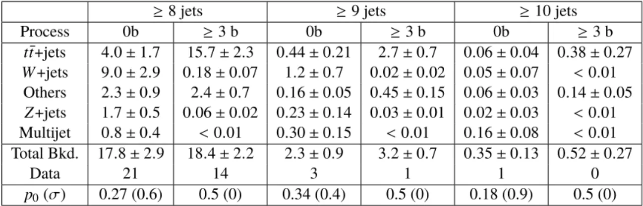
The model-independent test is used to search for, and to set generic exclusion limits on, the potential contribution of an unknown BSM signal in the phase-space region probed by this analysis. For this purpose, dedicated signal regions are defined which could be populated by such a possible signal, and where the SM contribution is expected to be small. The SR selections are defined as requiring exactly zero or at least three b -tags (labelled 0b, or 3b respectively) for a given minimum number of jets J, and for a jet p

threshold X, with each SR labelled as X-0b-J or X-3b-J. For each jet p

threshold six SRs are defined as follows:

• For the 40 GeV jet p

threshold: 40-0b-10, 40-3b-10, 40-0b-11, 40-3b-11, 40-0b-12, 40-3b-12.

• For the 60 GeV jet p

threshold: 60-0b-8, 60-3b-8, 60-0b-9, 60-3b-9, 60-0b-10, 60-3b-10.

• For the 80 GeV jet p

threshold: 80-0b-8, 80-3b-8, 80-0b-9, 80-3b-9, 80-0b-10, 80-3b-10.

The SRs therefore overlap and an event can enter more than one SR. Due to the efficiency of the b -tagging algorithm used, signal models with large b -tag multiplicities can have significant contamination in the two b -tag bins which can bias the t¯ t +jets background estimate reducing the sensitivity of the search. To reduce this effect, for the ≥ 3 b -tag SRs, the two b -tag bin is not included in the fit for the highest jet multiplicity slice in each SR.10

For the model-independent hypothesis tests, a separate likelihood fit is performed for each SR. A potential signal contribution is considered in the given SR bin only. The number of freely floating parameters of the background model is 15, whereas the number of observables varies between 23 (for SRs 60-3b-8 and 80-3b-8) and 45 (for SR 40-0b-12), hence, the system is also always over-constrained.

The fit setup has been extensively tested using MC simulated events, and has been demonstrated to give a negligible bias in the fitted yields, both in the case where the background-only distributions are fit, or when a signal is injected into the fitted data. These tests have been carried out with the nominal MC samples as well as the alternative samples described in Table 1. In addition when fitting the data the fitted parameter values and their inter-correlations were studied in detail and found to be in agreement with the expectation based on MC simulated event samples. The jet-reconstruction stability at high multiplicities has been

9For example, for the 60 and 80 GeV jetp_Tthresholds, there are fiveb-tag multiplicity bins in the eight-to-ten jet slices, and seven bins (the zerob-tag bin is split into three bins for each of theW/Zcontrol regions) in the five-, six- and seven-jet slices, giving 36 bins in total.

10For example, for the 0b-8 SRs all bins with five, six and seven jets will be included in the fit, as well as the one, two, three and four-or-moreb-tag bins with at least eight jets. Whereas for the 3b-8 SRs all bins with five, six and seven jets will be included in the fit, as well as the zero, and oneb-tag bins with at least eight jets.

validated by comparing jets with track-jets that are clustered from ID tracks with a radius parameter of 0.2.

The ratio of the multiplicities of track-jets and jets, which is sensitive to jet-merging effects, was found to be stable up to the highest jet multiplicities studied. The estimate of the multi-jet background has been validated in data regions enriched in FNP leptons, and been found to describe the data within the quoted uncertainties.

8 Systematic uncertainties

The dominant backgrounds are estimated from the data without the use of MC simulation, and therefore the main systematic uncertainties related to the estimation of these backgrounds arise from the assumptions made in the W /Z +jets, t¯ t +jets and multi-jet background estimates. Uncertainties related to the theoretical modelling of the specific processes and due to the modelling of the detector response in simulated events are only relevant for the minor backgrounds, which are taken from MC simulation, and for the estimates of the signal yields after selections.

For the W/Z +jets background estimation, the uncertainty related to the assumed scaling behaviour is taken from studies of this behaviour in W +jets and Z +jets MC simulation, as well as in γ +jets and multi-jet data control regions chosen to be kinematically similar to the search selection (see Figure 3). No evidence is seen for a deviation from the assumed scaling behaviour and the statistical precision of these methods is used as an uncertainty (up to 18% for the highest jet multiplicity bins). The expected uncertainty on the charge-asymmetry for W +jets production is 3 − 5% from PDF variations [83], but in the seven-jet region, the uncertainty is dominated by the limited number of MC events (up to 10% for the 80 GeV jet p

threshold). The uncertainty on the shape of the b -tag multiplicity distribution in W +jets and Z +jets events is derived by comparing different MC generator setups (e.g. varying the renormalisation and factorisation scale and the parton-shower model parameters). It is seen to grow as a function of jet multiplicity and is about 50% for events with five jets after which the MC statistical uncertainty becomes very large. An uncertainty of 100% is therefore assigned on the fractional contribution from W + b and W + c events for all jet multiplicity slices considered, which has a very small impact on the final result. In addition, the uncertainties related to the b -tagging efficiency and mis-tag rate are taken into account in the uncertainty on the W/Z +jets b -tag template.

The uncertainties related to the t t ¯ +jets background estimation primarily relate to the number of events in the data regions used for the fit. As mentioned in Section 6.2, the method shows good closure using simulated event samples, so no systematic uncertainty related to these studies is assigned. There is a small uncertainty related to the acceptance correction of the initial b -tag multiplicity template, which is derived by varying the MC generator setup for the t¯ t sample used to estimate the correction. This leads to a 3%

uncertainty on the correction and has no significant effect on the final uncertainty. The uncertainty related to the parameterization of the scaling of the t¯ t +jets background with jet multiplicity is determined with MC closure tests. The validation of the method presented in Figure 5 shows that the parameterization describes the data and MC well. The uncertainties assigned vary between 3% (at 8 jets) to 33% (at 12 jets) for the 40 GeV jet p

threshold, and 10% (at 8 jets) to 60% (at 10 jets) for the 80 GeV jet p

threshold.

These are taken by studying the closure of the method in different MC samples (including using alternative MC generators, and varying the event selection) and are of similar size to the statistical uncertainty from the data validation.

The dominant uncertainties on the multi-jet background estimate arise from the number of data events in

the control regions, uncertainties related to the subtraction of electroweak backgrounds from these control

regions (here a 20% uncertainty is applied on the expected yield of the backgrounds in the control regions) and uncertainties to cover the possible dependencies of the real- and fake- efficiencies [80] on variables other than lepton p

(for example the dependence on the number of jets in the event). The total uncertainty on the multi-jet background is about 50%.

The uncertainty on the expected yields of the minor backgrounds includes theoretical uncertainties on the cross-sections and on the modelling of the kinematics by the MC generator, as well as experimental uncertainties related to the modelling of the detector response in the simulation. The uncertainties assigned to cover the theoretical estimate of these backgrounds in the relevant regions are 50%, 100% and 30% for diboson, single top-quark, and t¯ tV /H production, respectively.

The systematic uncertainties related to the background estimation do not play a big role in the final uncertainty on the background estimates in the SRs, which are dominated by the statistical uncertainty related to the number of data events in the control regions.

The uncertainties assigned on the expected signal yield for the SUSY benchmark processes considered include the experimental uncertainties related to the detector modelling, which are dominated by the modelling of the jet energy scale, the jet energy resolution, and the b -tagging efficiencies and mis-tagging rates. The uncertainty on the signal cross-sections used is discussed in Section 3. The uncertainty on the signal yields related to the modelling of additional jet radiation is studied by varying the factorization, renormalization, and jet-matching scales as well as the parton-shower tune in the simulation. The corresponding uncertainty is small for most of the signal parameter space, but increases to up to 25% for very light or very heavy LSPs where the contribution from additional jet radiation is relevant.

9 Results

Results are provided both as model-independent limits on the contribution from BSM physics to the dedicated signal regions and in the context of the four SUSY benchmark models discussed in Section 3.2.1.

As previously mentioned, different fit setups are used for these two sets of results. In all cases the profile- likelihood-ratio test [84] is used to establish 95% confidence intervals using the CL

prescription [85].

Figures 6, 7 and 8 show the observed numbers of data events compared to the fitted background model,

for the three jet p

thresholds. The likelihood fit is configured using the model-dependent setup where all

bins are input to the fit, and fixing the signal strength parameter to zero. An example signal model is also

shown to illustrate the separation between the signal and the background achieved, as well as the level of

the leakage of the signal events into lower b -tag and jet-multiplicity bins. The bottom panel of each figure

shows the background prediction using MC simulation, which indicate for high b -tag multiplicities ( ≥ 3)

the MC simulation strongly underestimates the background contributions compared to the data-driven

background estimation. This effect has been observed before [86, 87] and shows that the MC simulations

are not able to correctly describe high b -jet multiplicity final states. In addition, the MC predicts too many

events at low b -jet multiplicity which is likely to be due to a mismodelling of the W +jets production at

high jet multiplicity. Since the background prediction from MC simulation does not reflect the expected

background contribution, in all cases the expected limit is computed using the background prediction from

a fit to all bins in the data with no signal component included in the fit model.