Origin of the gamma-ray emission in AGN jets
—
A multi-wavelength photometry and polarimetry data analysis of the quasar 3C 279
INAUGURAL-DISSERTATION
zur
Erlangung des Doktorgrades
der Mathemathisch-Naturwissenschaftlichen Fakult¨ at der Universit¨ at zu K¨ oln
vorgelegt von
Kiehlmann, Sebastian aus Moers, Deutschland
K¨ oln 2015
II
Berichterstatter: Prof. Dr. J. A. Zensus Prof. Dr. A. Eckart
Tag der m¨ undlichen Pr¨ ufung: 26. Juni 2015
Abstract
One of the main topics regarding the physics of AGN jets is the origin of the γ-ray emission. The favoured model explaining the production of high energy radiation in blazars is inverse Compton scattering. Though numerically and empirically successfully tested, two major questions remain topics of substantial discussion:
First, where is the seed photon field coming from? Does it originate in the jet itself (synchrotron self-Compton (SSC)) or in the accretion disc, the dust torus or the broad line region (external Compton (EC))? And second, where in the jet does the inverse Compton scattering take place?
This thesis aims to locate the γ-ray emission site in the archetypical blazar 3C 279 based on the multi-frequency photometry data provided by the Quasar Movie Project. This data set includes 140 light curves at more than twenty bands, providing dense sampling in frequency and time domain over more than two years.
These data allow us to analyse the variability of the light curves and to perform cross- correlation analysis over a large range of frequencies. We estimate the variability power spectra at 26 frequencies. We find similar indices of a power-law spectrum at sub-mm bands and X-rays on the one hand, and at ultraviolet and γ-rays on the other hand. Additionally, we find a strong correlation between X-rays and the 1 mm light curve at short variability time scales. We can infer that the X-ray emission site is located at the mm VLBI core and that X-rays are produced either by synchrotron self-Compton scattering of mm-wavelength synchrotron photons or by external Compton scattering of photons originating from the cosmic microwave background. The correlation between X-rays, γ-rays, and optical bands exhibits complex behaviour. Time lags between the bands change over time, indicating probably different emission sites and different physical conditions. But we find some indication that the γ-ray emission site is located, at least occasionally, at the mm VLBI core. Thus, it is located beyond the broad line region, where infrared photons either from the jet itself or from the dust torus may serve as seed photons for the inverse Compton scattering to GeV energies.
Another major topic of ongoing discussion regards the structure of the magnetic field in the jets. The observed synchrotron radiation in the spectral regime from radio to x-rays and the polarization of the radiation are direct evidence for the existence of magnetic fields in the jets. Furthermore current jet models require magnetic fields to explain the launching and acceleration of jets. But the structure of the magnetic field is unknown. Long, smooth continuous variation of the electric vector position angle (EVPA) and very long baseline interferometry (VLBI) rotation measure studies indicate helical magnetic field structures. Whereas erratic EVPA variation indicates a tangled magnetic field structure and shocks traversing a turbulent medium may temporarily order the tangled magnetic field to produce smooth EVPA changes.
The combined optical polarimetry data provided by the Quasar Movie Project yields an unprecedentedly well sampled polarization curve of 3C 279 which shows
III
IV
strong variability with rotations of the polarization angle in both directions with different rotation rates and amplitudes. We introduce various, new methods to analyse the polarization variability. We test different classes of stochastic models against the observed data and come to the conclusion that the polarization variability of 3C 279 is following two different processes. During a low brightness state the polarization is consistent with a stochastic process. During a flaring state the variability is dominated by a different process. The preferred model is that of an emission feature on a helical path in a helical magnetic field.
Kurzzusammenfassung
Die Frage nach dem Ursprung der γ-Strahlung ist eines der wesentlichen Themen auf dem Gebiet der Physik aktiver Galaxienkerne. Inverse Compton-Streuung ist das bevorzugte Modell, um die Erzeugung von hochenergetischer Strahlung in Blazaren zu erkl¨aren. Obwohl dieses Modell numerisch und empirisch erfolgreich getestet ist, bleiben zwei wesentliche Fragen bislang offen: Erstens, woher stammen die urspr¨unglichen Photonen, die zu h¨oherer Energie gestreut werden? Werden diese im Jet selbst erzeugt (synchrotron Selbst-Compton (SSC)-Streuung), oder stammen sie aus einer externen Region (externe Compton (EC)-Streuung) wie der Akkretionsscheibe, dem Staubtorus oder der Broad Line Region? Zweitens, wo im Jet findet der Streuprozess statt?
Diese Doktorarbeit versucht das Emissionsgebiet der γ-Strahlung im Blazar 3C 279 anhand von photometrischen Daten, beobachtet bei einer Vielzahl von Frequenzen, zu lokalisieren. Diese Daten werden durch das Quasar Movie Project zur Verf¨ugung gestellt und beinhalten 140 Lichtkurven bei ¨uber zwanzig Frequenzen.
Damit bietet der Datensatz eine hohe Abtastrate sowohl im Zeit-, wie im Fre- quenzbereich ¨uber einen Zeitraum von ¨uber zwei Jahren. Diese Daten erm¨oglichen es die Variabilit¨at der Lichtkurven zu untersuchen und eine Kreuzkorrelationsanalyse
¨
uber einen großen Frequenzbereich durchzuf¨uhren. Wir sch¨atzen die spektralen En- ergiedichte der Lichtkurvenvariation in 26 verschienden Frequenzba¨ndern ein. Zum Einen finden wir eine vergleichbare Verteilung der Energiedichte f¨ur die R¨ontgen- und die sub-mm-Strahlung, zum Anderen eine vergleichbare Verteilung f¨ur die ultraviolette und die γ-Strahlung. Zudem zeigt sich eine starke Korrelation zwis- chen der Kurzzeitvariabilit¨at der R¨ontgenstrahlung und der mm-Strahlung. Daraus schließen wir, dass die R¨ontgenstrahlung in der N¨ahe des mm-VLBI-Kernes erzeugt wird, entweder durch Selbst-Compton-Streuung von mm-Synchrotronstrahlung oder durch externe Compton-Streuung von Photonen der kosmischen Mikrowellenhin- tergrundstrahlung. Die Korrelation zwischen γ-Strahlung, R¨ontgenstrahlung und optischer Strahlung zeigt ein komplexes Verhalten. Die Verz¨ogerungen der Variation zwischen verschiedenen Frequenzbereichen sind zeitlich variable. Dieses Verhal- ten ist m¨oglicherweise ein Hinweis darauf, dass diese Strahlung an verschiedenen Stellen, unter unterschiedlichen physikalischen Bedingungen erzeugt wird. Dennoch finden wir Anzeichen daf¨ur, dass das Emissionsgebiet der γ-Strahlung, zumindest zeitweilig, mit der Position des mm VLBI Kernes ¨ubereinstimmt. Damit liegt das Emissionsgebiet außerhalb der Broad Line Region. Somit kommen als urspr¨ungliche Photonen f¨ur die inverse Compton-Streuung zu h¨oherer Energie lediglich Strahlung im Infrarotbereich in Frage, welche entweder im Jet selbst oder vom Staubtorus emittiert wird.
Ein weiteres Thema andauernder Diskussion betrifft die Struktur des Magnet- feldes im Jet. Die beobachtete Synchrotronstrahlung ¨uber das gesamte Spektrum vom Radiobereich bis hin zur R¨ontgenstrahlung und die kennzeichnende Polarisa- tion dieser Strahlung ist ein direkter Beweis f¨ur die Existenz von Magnetfeldern
V
VI
in Jets. Des Weiteren sind Modelle, die aktuell zur Erkl¨arung des Usprunges und der Beschleunigung von Jets herangezogen werden, wesentlich auf die Existenz von Magnetfeldern angewiesen. Dennoch ist die Struktur der Magnetfelder bislang unbekannt. Lange, kontinuierliche und glatte Verl¨aufe, die die Ver¨anderung des Polarisationswinkels anzeigen sowie Messungen der Faraday-Rotation auf Basis von VLBI-Daten deuten auf eine Helixstruktur des Magnetfeldes hin. Die sprunghafte Variation des Polarisationswinkels wiederum deutet auf ein chaotisches Magnetfeld.
Dieses ungeordnete Magnetfeld kann durch eine Schockfront, die das turbulente Medium durchl¨auft, kurzweilig komprimiert werden und dadurch geordnet er- scheinen. Dies kann auch bei einer chaotischen Magnetfeldstruktur zu glatten Verl¨aufen der Polarisationswinkelver¨anderung f¨uhren.
Die kombinierten Polarisationsdaten im optischen Frequenzbereich, die durch das Quasar Movie Project bereitgestellt werden, bilden die Polarisationsvariation von 3C 279 mit sehr hoher zeitlicher Abtastrate ab. Diese Daten zeigen eine hohe Variabilit¨at des Polarisationswinkels. Rotationen in beide Richtungen treten auf mit variierenden Rotationsgeschwindigkeiten und -amplituden. Wir stellen verschiedene, neue Methoden vor, um Polarisationsdaten zu analysieren. Wir testen unterschiedliche Klassen von stochastischen Prozessen gegen die Daten und schlussfolgern, dass 3C 279 zwei verschiedenen Prozessen unterworfen ist, die die Variation der Polarisation erkl¨aren. Im Zustand geringer Intensit¨at ist die Po- larisationsvariation konsistent mit einem stochastischem Prozess. Wiederum im Zustand starker Intensit¨atsausbr¨uche kann die Variation nicht durch einen der hier beschriebenen stochastischen Prozesse beschrieben werden. Das bevorzugte Modell, welches die Variation in diesem Zustand beschrieben kann, ist das eines Emis- sionsgebietes, welches sich auf einer spiralf¨ormigen Bahn durch ein spiralf¨ormiges Magnetfeld bewegt.
Contents
1 Introduction 1
1.1 Active galactic nuclei . . . 1
1.1.1 Historical review of AGN observations . . . 1
1.1.2 Unified AGN model and radiation processes . . . 2
1.1.3 AGN classification . . . 4
1.2 Blazars . . . 5
1.2.1 Relativistic effects . . . 5
1.2.2 Jet launching, acceleration and collimation . . . 7
1.2.3 Spectra and emission processes . . . 7
1.2.4 Polarization . . . 10
1.3 The Quasar Movie Project . . . 11
1.4 3C 279 . . . 11
2 Photometry data 15 2.1 Data processing methods: . . . 15
2.1.1 Cross-calibration . . . 15
2.1.2 Iterative averaging . . . 18
2.1.3 Extinction correction . . . 19
2.1.4 Flux scale conversion . . . 20
2.2 Radio, mm and sub-mm data . . . 21
2.3 Infra-red, optical, and ultraviolet data . . . 21
2.4 X-ray data . . . 25
2.5 Gamma-ray data . . . 27
2.6 The final multi-wavelength data set . . . 28
3 Multi-wavelength flux variability 31 3.1 3C 279 light curves . . . 31
3.2 Estimation of the light curve probability density functions . . . 33
4 Power spectral densities 37 4.1 Estimation of the raw power spectrum . . . 37
4.1.1 The necessity of a window function . . . 38
4.1.2 Red noise leakage and linear de-trending . . . 40
4.1.3 Aliasing . . . 42
4.1.4 Splitting and re-sampling the data . . . 45
4.2 Light curve simulation . . . 46
4.2.1 Generating Gaussian noise . . . 46
4.2.2 Fitting the spectral amplitude . . . 48
4.2.3 Matching the light curve variance . . . 49
4.2.4 Generating noise following both the desired Power Spectral Density (PSD) and Probability Density Function (PDF) . . 49
VII
VIII CONTENTS
4.2.5 Stability of the spectral index . . . 50
4.2.6 Re-sampling and re-binning to uneven grid . . . 51
4.2.7 Error simulation . . . 53
4.2.8 Light curve simulation for PSD estimation . . . 53
4.3 Estimation of the intrinsic power spectrum . . . 54
4.3.1 Best model parameter . . . 54
4.3.2 p-value and confidence interval . . . 55
4.3.3 Reliability test . . . 56
4.4 B-band and 9 mm-band power spectral analysis . . . 57
4.5 Multi-wavelength power spectral analysis . . . 62
4.6 Stationarity . . . 66
4.7 Summary of the PSD analysis . . . 67
5 Cross-correlation analysis 71 5.1 Methods of the cross-correlation analysis . . . 71
5.1.1 Estimation of the cross-correlation function . . . 71
5.1.2 Significance of the cross-correlation function . . . 73
5.1.3 Time lag uncertainty . . . 77
5.2 DCF analysis . . . 78
5.2.1 Cross-correlation of the radio bands . . . 78
5.2.2 Cross-correlation of the ultraviolet, optical, infrared bands . 83 5.2.3 Cross-correlation of best sampled light curves . . . 84
5.3 Summary of the correlation analysis . . . 95
6 Polarization 99 6.1 Introduction to polarization and polarimetry . . . 99
6.2 Polarimetry data . . . 101
6.3 EVPA ambiguity . . . 103
6.3.1 Reliability of the Electric Vector Position Angle (EVPA) adjustment . . . 105
6.4 Optical EVPA variation of 3C 279 . . . 109
6.5 mm and cm EVPA variation of 3C 279 . . . 112
6.6 EVPA variation estimator . . . 113
6.6.1 Error bias of the variation estimator . . . 114
6.6.2 Curvature bias of the variation estimator . . . 117
6.7 EVPA rotation identification . . . 119
6.7.1 Rotation identification algorithm . . . 119
6.7.2 Testing the rotation identification . . . 121
6.8 Polarization properties of 3C 279 . . . 122
7 Random walk polarization model 129 7.1 Definition of the random walk models . . . 129
7.1.1 Randomized time sampling . . . 129
7.1.2 Simple Q, U random walk process . . . 130
7.1.3 Shock Q, U random walk process, I uniform . . . 131
7.1.4 Shock Q, U random walk process, I decreasing . . . 131
7.1.5 Integrated polarization . . . 132
7.1.6 Simulated EVPA errors . . . 132
7.1.7 Prior distribution selection . . . 133
7.2 Model analysis . . . 134
7.2.1 Dependency on input parameters . . . 135
CONTENTS IX
7.2.2 Dependencies between measured parameters . . . 140
7.2.3 Model comparison . . . 141
7.3 Expectation values of the fractional polarization . . . 146
7.4 Test random walk polarization models against observations . . . 148
7.4.1 Period IIa: parameter distributions . . . 148
7.4.2 Period IIa: probability . . . 153
7.4.3 Period IIIc: parameter distributions . . . 155
7.4.4 Period IIIc: probability . . . 158
7.5 Distribution of rotation amplitudes . . . 158
7.6 Conclusion: two classes of processes . . . 161 8 Deterministic polarization variation models 163
9 Summary and outlook 167
X CONTENTS
List of Figures
1.1 Sketch of the unified AGN model. . . 2
2.1 Illustration of the averaging algorithm. . . 18
2.2 Colour indices of 3C 279 . . . 25
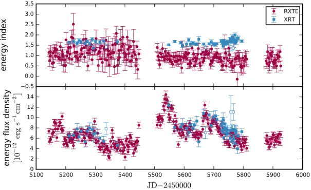
2.3 RXTE-PCA and Swift-XRT light curve of 3C 279 . . . 27
3.1 3C 279 light curves. . . 32
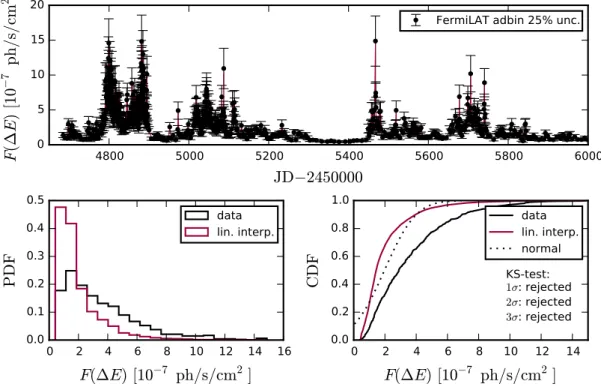
3.2 PDF of the gamma-ray light curve. . . 35
3.3 PDF of the X-ray light curve. . . 35
3.4 PDF of the V-band light curve. . . 36
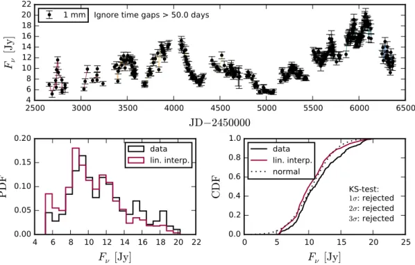
3.5 PDF of the 1 mm light curve. . . 36
4.1 Comparison of periodogram and LSP spectral index estimates. . . . 39
4.2 Comparison of PSD indices with and without window function. . . 39
4.3 Influence of red noise leakage on the PSD index estimation. . . 41
4.4 Illustration of low frequency variability. . . 42
4.5 Influence of de-trending on the PSD index estimation. . . 43
4.6 Influence of aliasing on the PSD index estimation. . . 44
4.7 Spectral index stability of light curve simulations. . . 52
4.8 Example PSD estimation: light curves. . . 57
4.9 Example PSD estimation: raw periodogram and model. . . 58
4.10 Example PSD estimation: χ2-minimization. . . 58
4.11 Example PSD estimation: p-value. . . 59
4.12 Example PSD estimation: confidence interval. . . 59
4.13 Example PSD estimation: accuracy. . . 60
4.14 Example PSD estimation: false negatives. . . 60
4.15 Example PSD estimation: confidence limit accuracy. . . 61
4.16 Raw and intrinsic power spectra of 3C 279. . . 68
4.17 Frequency dependent power spectral indices of 3C 279. . . 69
4.18 Long and short term X-ray variability. . . 69
4.19 V-band light curve of 3C 279 . . . 70
5.1 Simulatedγ-ray light curves. . . 75
5.2 Simulated V-band light curves. . . 75
5.3 Simulated 21 mm light curves. . . 75
5.4 Auto-correlation function of the γ-ray light curve. . . 76
5.5 Auto-correlation function of the V-band light curve. . . 76
5.6 Auto-correlation function of the 21 mm light curve. . . 76
5.7 CCPD of the V-band ACF. . . 79
5.8 CCPD of the 21 mm ACF. . . 79
5.9 Relative cm, mm, sub-mm correlation time lags. . . 80 XI
XII LIST OF FIGURES
5.10 Correlation of X-rays and 1 mm band. . . 85
5.11 Correlation of de-trended X-ray and 1 mm light curves. . . 85
5.12 Correlation of smoothed X-ray and 1 mm light curves. . . 86
5.13 Correlation of V-band and 21 mm band. . . 87
5.14 Correlation of V-band and 8 mm band. . . 87
5.15 Correlation of V-band and 1 mm band. . . 88
5.16 Correlation of V-band and 870µm band. . . 88
5.17 Correlation of smoothed V-band and 21 mm band. . . 90
5.18 Correlation of de-trended V-band and 21 mm band. . . 90
5.19 Time shifted X-ray and V-band light curves. . . 91
5.20 Correlation of γ-rays and V-band. . . 93
5.21 Correlation of de-trended γ-rays and V-band. . . 94
5.22 Time shiftedγ-ray and V-band light curves. . . 95
5.23 Time shifted X-ray, V-band, and γ-ray light curves. . . 96
6.1 EVPA consistency level. . . 106
6.2 Probability of correct EVPA reconstruction. . . 107
6.3 EVPA consistency level and reliability limits. . . 108
6.4 EVPA reconstruction consistency and reliability. . . 110
6.5 Combined optical EVPA curve of 3C 279. . . 110
6.6 EVPA of 3C 279 at mm and cm frequencies. . . 112
6.7 Manually adjusted mm EVPA of 3C 279. . . 113
6.8 EVPA variation estimator error bias. . . 115
6.9 Observational error bias of the EVPA variation estimator. . . 116
6.10 De-biasing of the EVPA variation estimator. . . 117
6.11 EVPA variation estimator curvature bias. . . 118
6.12 Testing the EVPA rotation identification. . . 122
6.13 Optical polarization of 3C 279. . . 123
6.14 EVPA variation estimator of 3C 279. . . 124
6.15 Identified rotations in the 3C 279 EVPA curve. . . 125
6.16 Number of identified EVPA rotations for 3C 279. . . 125
7.1 Illustration of the Stokes Q-U-normalization. . . 131
7.2 Random walk polarization model prior distribution. . . 134
7.3 Random walk model dependency on prior distribution. . . 134
7.4 Model parameter dependence: mean polarization fraction. . . 136
7.5 Model parameter dependence: polarization fraction standard deviation.136 7.6 Random walk parameter dependence: EVPA amplitude. . . 138
7.7 Model parameter dependence: EVPA rotation rate. . . 138
7.8 Model parameter dependence: EVPA variation estimator. . . 139
7.9 Model parameter dependence: number of EVPA rotations. . . 139
7.10 Model parameter dependence: EVPA adjustment consistency. . . . 140
7.11 Random walk model: dependencies between measured parameters. . 141
7.12 Model distributions of the mean polarization fraction. . . 142
7.13 Model cell number dependency of the polarization fraction distribution.142 7.14 Model distributions of the polarization fraction standard deviation. 143 7.15 Model distributions of the EVPA amplitude. . . 143
7.16 Model cell number dependency of the EVPA amplitude distribution. 143 7.17 Model distributions of the EVPA rotation rate. . . 144
7.18 Model distributions of the EVPA variation estimator. . . 144
7.19 Model distributions of the EVPA rotation number. . . 145
LIST OF FIGURES XIII
7.20 Model distributions of the EVPA consistency. . . 145
7.21 Model distributions of the mean polarization fraction (2). . . 146
7.22 Model distributions of the polarization fraction standard deviation (2).147 7.23 Polarization fraction expectation values. . . 147
7.24 Best model parameters: period IIa polarization selected (1). . . 149
7.25 Best model parameters: period IIa polarization selected (2). . . 150
7.26 Best model parameters: period IIa polarization selected (3). . . 150
7.27 Period IIa polarization variation distribution. . . 150
7.28 Best model parameters: period IIa EVPA selected. . . 151
7.29 Period IIa EVPA amplitude distribution. . . 152
7.30 Period IIa EVPA variation distribution. . . 152
7.31 Best model parameters: period IIa polarization and EVPA selected. 152 7.32 Best model parameters: period IIa polarization and EVPA selected (2). . . 153
7.33 Period IIa observation probability. . . 155
7.34 Period IIa observation probability (2). . . 155
7.35 Best model parameters: period IIIc polarization selected. . . 156
7.36 Period IIIc polarization variation distribution. . . 156
7.37 Period IIIc EVPA amplitude distribution. . . 157
7.38 Period IIIc EVPA variation distribution. . . 157
7.39 Best model parameters: period IIIc EVPA selected. . . 157
7.40 Period IIIc observation probability. . . 158
7.41 Rotation amplitude distribution of 3C 279. . . 159
7.42 Rotation amplitude distribution of the random walk models. . . 160
7.43 Model against observed rotation amplitude distribution. . . 160
8.1 Two-component polarization swing. . . 164
XIV LIST OF FIGURES
List of Tables
2.1 Quasar Movie Project photometry observations. . . 16
2.2 Optical and infra-red filter properties. . . 20
2.3 UVOT filter properties. . . 20
2.4 Sub-mm, mm, and cm cross-calibration factors. . . 22
2.5 Optical and infrared cross-calibration offsets. . . 26
2.6 Final Quasar Movie Project photometry data set and time sampling. 29 4.1 Results of the power spectral index estimation. . . 64
4.2 Time resolved power spectral indices of the V-band light curve. . . 66
5.1 Cross-correlation time lags at cm, mm, sub-mm bands. . . 81
5.2 Cross-correlation time lags between short term X-ray and mm, cm variability. . . 85
5.3 Time lags between V-band and radio bands. . . 89
6.1 Quasar Movie Project polarimetry observations. . . 101
6.2 Final Quasar Movie Project polarization data set and time sampling.103 6.3 Optical EVPA variation of 3C 279. . . 111
6.4 Overview over the rotation identification algorithm. . . 127
6.5 Optical polarization characteristics of 3C 279. . . 128
6.6 Time sampling model parameters. . . 128
6.7 EVPA uncertainty modelling parameters. . . 128
6.8 Frequency dependent polarization fraction of 3C 279. . . 128
7.1 Period IIa model probability and optimal parameters. . . 154
7.2 Period IIa model probability and optimal parameters (2). . . 155
XV
XVI LIST OF TABLES
Chapter 1 Introduction
1.1 Active galactic nuclei
An active galaxy is a special subtype of galaxy which is characterized by its central region, the Active Galactic Nucleus (AGN). Many different classes of extragalactic astrophysical objects are summarized under the term AGN. Those classes, initially interpreted as different kinds of objects but nowadays unified in the model of an AGN, evolved out of various classification schemes and observations at different frequency ranges. Though historically evolved and revised as a single type of object, these classifications are still in use to distinctively characterize subclasses of AGN.
1.1.1 Historical review of AGN observations
Messier 77 (NGC 1068) was the first object, reported in 1909 by Edward Fath, which was later on classified as AGN. The spectrum of this spiral nebula1 showed emission lines, an unprecedented result at that time (Fath, 1909).
The first systematic study of spectral lines in extragalactic objects was conducted by Seyfert (1943), describing broad and narrow emission lines and absorption lines in various extragalactic nebulae. The fact that not all objects showed broad emission lines led to the first classification into Seyfert 1 galaxies and Seyfert 2 galaxies.
In the 1950s radio astronomy started as a new branch of astronomy and the first systematic radio surveys led to a large number of newly found radio emitting objects listed in the Third Cambridge Catalogue of Radio Sources (3C).
Gradually, many of the 3C objects were identified with known astrophysical objects previously observed in optical bands, for instance Cygnus A (3C 405) (Baade and Minkowski, 1954), 3C 273 (Schmidt, 1963), and 3C 48 (Matthews and Sandage, 1963). The spectra of the optical counterparts showed high redshift, indicating that these radio sources were extragalactic objects. Later on the termsradio galaxy for extended extragalactic radio sources (e.g. Cynus A) and quasar or quasi-stellar radio source for point-like sources were established. The class of quasars was generalized to Quasi-Stellar Objects (QSOs) once several point-like optical sources
1Nebulous objects, differing from point-like stars, are recorded since the 10th century (Book of Fixed Stars by Abd al-Rahman al-Sufi) but first in the early 20th century with spectrographic studies in the 1910s began the discussion that the stars observed were located in a closed system, the Milky Way, and that those nebulae were located far outside of the Milky Way. Within this scientific process, including the Great Debate between Harlow Shapley and Heber Curtis and leading up to Edwin Hubble‘s classification of galaxy morphologies, spiral nebulae were first renamedisland universes and latergalaxies.
1
2 CHAPTER 1. INTRODUCTION consistent with the optical spectra of quasars but without radio emission were identified. Morphology studies of the extended radio emission from AGN led to the classification into FR-I and FR-II sources (Fanaroff and Riley, 1974).
With the Einstein Observatory (HEAO-2) (1978-1982) and later on ROSAT (1990-1999), RXTE (1995-2012), Chandra (since 1999), XMM-Newton (since 1999),
and Swift (since 2004) AGN were also identified as X-ray sources. With the Energetic Gamma Ray Experiment Telescope (EGRET) on the Compton Gamma Ray Observatory satellite operating between 1991 and 2000 some AGN were furthermore identified as γ-ray sources (von Montigny et al., 1995) which are continuously monitored since 2008 with the Large Area Telescope (LAT) on the Fermi satellite. Punch et al. (1992) showed that the emission of Mrk 421 reaches up to TeV-energy, observed with the Whipple 10 m gamma-ray telescope using the the Imaging Atmospheric Cherenkov Technique. With the successors VERITAS and MAGIC more TeV-sources have been identified amongst the AGN.
Antonucci and Miller (1985) showed that the Seyfert 2 galaxy Messier 77 (NGC 1068) showed characteristics of a Seyfert 1 galaxy in polarized light. In the late 1980s to early 1990s the scientific discussion led to the unified model of AGN (Urry and Padovani, 1995, and references therein).
1.1.2 Unified AGN model and radiation processes
Figure 1.1: Sketch of the unified AGN model with a central SMBH (black) sur- rounded by an accretion disc (red) and a dust torus (brown). Gas clouds in the BLR (dark blue) are located inside the dust torus, gas clouds in the NLR (pale blue) outside. A jet (orange) does not occur in all AGN (Sketch by S. Kiehlmann, based on Urry and Padovani, 1995).
Figure 1.1 shows a sketch of the unified AGN model containing a SMBH, an accretion disc, a dust torus, gas clouds in the BLR and NLR, and in the case of a radio-loud AGN a jet. The AGN itself is located in the centre of a host galaxy. All components contribute differently to the overall electromagnetic spectrum of the AGN.
The largely accepted model assumes a SMBH at the very centre of the AGN.
The order of the central black hole mass typically ranges from 106 to 1010 solar masses. The SMBH is surrounded by an accretion disc feeding the black hole. This system of SMBH and accretion disc is occasionally referred to as the central engine
1.1. ACTIVE GALACTIC NUCLEI 3 of an AGN. Due to friction, angular momentum of the gas is transported outward and the gas is moving to lower orbits around the black hole down to the Innermost Stable Circular Orbit (ISCO) below which the gas plunges into the black hole.
While moving inward the gas looses potential energy and heats up. Consequentially, the accretion disc producesthermal radiation. The temperature of the disc is higher at smaller radii. Thus, the emission of the disc can be modelled as a series of black body radiators integrated over the whole temperature distribution of the disc. The thermal emission from the disc typically ranges from optical to ultraviolet or soft X-rays and peaks at ultraviolet frequencies. This contribution to the overall AGN spectrum is often referred to as the Big Blue Bump.
An outflow of disc material may be launched either thermally, radiation pressure driven, or magnetically driven, known as disc wind. This material can absorb radiation, appearing as blue shifted Broad Absorption Lines (BAL) if the motion of the wind has a fast component towards the observer.
The accretion disc is surrounded by a dust torus. While it is usually referred to as torus the actual shape and structure is not well determined. The dust torus is emitting thermal radiation peaking at infra-red frequencies, referred to as the IR bump in AGN spectra. The torus is opaque at optical frequencies.
The black hole is additionally surrounded by clouds of gas. This gas is excited by the radiation coming from the disc and then produces emission lines in the optical and ultraviolet range, when the atoms fall back to lower energy levels. As these gas clouds are circulating around the SMBH the emission is Doppler shifted and the integration over the total range of velocity components along the line of sight leads to a broadening of the observed emission lines. The location of those gas clouds producing emission lines is divided into two regions: the broad and the narrow line region. The BLR is close to the central black hole, at ∼1 parsec distance, within the range of the dust torus. The width of the emission lines, typically measured in velocities corresponding to the circular motion of the gas clouds, ranges from 1000 to 10 000 kilometres per second. Depending on the orientation of the AGN towards the observer the BLR and the accretion disc may be obscured by the dust torus and no broad emission lines are visible in photometric spectra. Nevertheless, these broad lines may be visible in polarized light when scattered off the dust torus towards the observer. The scattering introduces the polarization of the light.
The NLR is located beyond the dust torus, at an estimated distance of 10 to 1000 parsecs from the SMBH, and thus is never obscured. Narrow emission lines have a width of <1000 kilometres per second. The gas density in the NLR is low enough to produce forbidden emission lines (e.g. [O III]). Forbidden lines always appear as narrow, never as broad lines. An observed broad emission line is usually a superposition of a narrow line component from the NLR, a broad line component from the BLR, and potentially a very broad, probably double-peaked component from the accretion disc.
A fraction of AGN produces relativistic jets. These outflows of matter extend far beyond the nucleus and even the host galaxy with sizes up to mega-parsecs.
These jets emit synchrotron radiation from radio up to optical, ultraviolet, or even X-rays. The most energetic jets additionally produce X-ray and γ-ray emission, occasionally up to TeV-energy. We discuss the jet emission processes in more detail in section 1.2.
With bolometric luminosities typically about 1044 to 1048 erg/s, AGN often outshine their host galaxies. Nevertheless, for the less luminous AGN the host galaxy consisting of stars and gas may contribute significantly to the observed
4 CHAPTER 1. INTRODUCTION spectrum.
This unified model of AGN can explain all typical characteristics of the many historically evolved sub-classes. The central engine, i.e. the SMBH and the accretion disc, is capable of maintaining the high energy output over long time scales with rapid variability at the same time. The different types of emission lines are explained by the gas clouds in the NLR and BLR, whereas the presence or absence of broad emission lines is related to dust torus which may or may not obscures the BLR and accretion disc depending on the orientation of the AGN with regard to the observer. Radio and γ-ray emission is explained by the presence of a relativistic jet.
1.1.3 AGN classification
The two main classifications of AGN are based on the optical and radio properties.
The optical classification differs between Type 1 AGN, which show broad (≥
1000 km/s) emission lines in the optical and ultraviolet spectral range, and Type 2 AGN, which do not show broad emission lines. The radio classification differs between AGN which do and do not show strong radio emission compared to the optical emission. AGN with flux density at 5GHz at least ten times larger than the flux density at R-band, f5 GHz ≥ 10fR, are called radio-loud, and radio-quiet otherwise. Most of the AGN are radio-quiet (80 % - 85 %, Kellermann et al. (1989)).
Seyfert 1 galaxies are radio-quiet Type 1 AGN. They show narrow and broad emission lines. Seyfert 2 galaxies exhibit only narrow emission lines. In the unified model the system is seen relatively edge-on (regarding to the accretion disc) and the BLR and the accretion disc are hidden behind the dust torus. A broad line component may be visible in polarized light, when the spectral line emission is scattered at the backside of the torus towards the observer (e.g., NGC 1068, Antonucci and Miller (1985)). Generally, Seyfert galaxies have relatively low luminosity. Therefore, only close by Seyfert galaxies are visible and, consequentially, the host galaxy can be resolved. Seyfert are generally hosted in spiral galaxies.
D. Osterbrok introduced a more detailed sub-classification of Seyfert galaxies into classes 1.2, 1.5, 1.8, 1.9 based on the relative strength of the narrow and broad components of the Balmer lines.
Radio-quiet QSOs (orradio-quiet quasars) are Type 1 AGN more luminous and at further distance than Seyfert 1 galaxies, otherwise there is no clear distinction between the two classes. The host galaxies of radio-quiet QSOs are unresolved and outshone by the nucleus.
LINER galaxies or LINERs (Low-ionization nuclear emission-line region) show emission lines from weakly ionized or neutral atoms. In contrast to Seyfert galaxies and QSOs highly ionized emission lines are rare. Consequentially, the power of the exciting source is significantly lower in LINERs. Due to the similarity of showing emission lines LINERs are often regarded to as AGN although it is still under debate if the source of energy is a SMBH with an accretion disc.
AGN with broad absorption lines (BALs) in optical and ultraviolet are classified asBAL quasars. Broad absorption lines are probably due to fast disc winds and may occur in Type 1 and Type 2 AGN.
The radio-loud counterpart to Seyfert 2 galaxies areNarrow Line Radio Galaxies (NLRG). They show the same optical properties as Seyfert 2 and additionally strong radio emission. Accordingly, Broad Line Radio Galaxies (BLRG) are radio-loud Type 1 AGN with the same optical properties as Seyfert 1 galaxies. Radio-loud
1.2. BLAZARS 5 QSOs or quasars2 are more luminous than BLRG. The luminosity distinction is
not clearly defined and there is no further difference between the two classes.
Depending on the radio synchrotron spectrum, which can be described as a power-law function Fν ∝ ν−α with spectral index α, the radio-loud quasars are further subdivided into Flat Spectrum Radio Quasars (FSRQ) for α ≤ 0.5 and Steep Spectrum Radio Quasars (SSRQ) for α > 0.5. Flat Spectrum Radio Quasars (FSRQs) are highly variable throughout the entire spectrum, highly polarized at radio and optical frequencies and the extended radio emission region is dominated by a compact radio core. Thus, classifications as Optically Violently Variable (OVV) quasar, Highly Polarized Quasar (HPQ), and Core Dominated Quasar (CDQ) refer to the same type of object as the term FSRQ and vice versa.
BL Lac objects, named after their prototype BL Lacertae, show similar charac- teristics as FSRQs, namely high luminosity, strong variability, high polarization.
The main observational difference is that BL Lac objects lack strong emission and absorption lines. Therefore, BL Lacs cannot be identified as Type 1 or Type 2 AGN.
BL Lacs and FSRQs, collectively, are called blazars. In the picture of the unified model they have jets closely aligned with the line of sight and thus differ from other radio-loud AGN only by orientation. Relativistic effects explain the extreme luminosity (Doppler boosting) and fast variability (time compression). The entire spectrum is dominated by emission from the jet, resulting in high polarization in radio and optical bands due to synchrotron emission. BL Lacs are expected to be intrinsically weak, FSRQs intrinsically strong AGN. We describe the physical properties of blazars in more detail in section 1.2.
With radio interferometry an extended radio emitting region can be resolved for many radio-loud AGN, some of which show a two-sided jet. Those sources are additionally classified based on the morphology of the extended emission region (Fanaroff and Riley, 1974). If the separation of the two brightest points – one on each side of the central jet emitting source – is less than half the size the entire radio structure the source is classified as Fanaroff-Riley Class I (FR-I) otherwise as Fanaroff-Riley Class II (FR-II). FR-II sources are generally more luminous than FR-I sources at radio frequencies and FR-II jets are generally more collimated than FR-I jets.
1.2 Blazars
Blazars are radio-loud AGN with a relativistic jet closely aligned with the line of sight. Blazars include the FSRQs and the intrinsically less powerful BL Lac objects.
Blazars typically show strong variability throughout the entire electromagnetic spectrum at time scales from hours to years (e.g. Gupta et al., 2008; Abdo et al., 2010b; Fuhrmann et al., 2014; Hayashida et al., 2015). Blazars are highly polarized in radio and optical (e.g. Agudo et al., 2014; Pavlidou et al., 2014).
1.2.1 Relativistic effects
The extreme luminosity and short time scales of variability can be (partially) attributed to relativistic effects. If an emission region in the jet moves with speed
2The termsQSO andquasar are often used interchangeably. Although quasar initially meant quasi-stellar radio source, equal to the termradio-loud QSO, it is also occasionally used in the termradio-quiet quasar instead of radio-quiet QSO. Therefore, it is recommendable to use the termradio-loud QSO or radio-loud quasar instead ofquasar to avoid ambiguity.
6 CHAPTER 1. INTRODUCTION v, the normalized speed is given as:
β = v
c ≤1, (1.1)
where c is the speed of light. We point out that β is the normalized speed of the bulk motion and not of an individual particle. The corresponding bulk Lorentz factor is:
Γ = 1
p1−β2 ≥1. (1.2)
With the angle between the jet flow direction and the line of sightθ the Doppler factor is given as:
δ= 1
Γ(1−βcosθ) ≥1 (1.3)
The Lorentz transformation from the rest frame of the emission region to the observer frame introduces various relativistic effects. As a result of time dilation the time scale of an observed event ∆tobs is shorter than the time scale ∆tem at which the event happens in the rest frame of the emission region:
∆tobs = ∆temδ−1. (1.4)
Accordingly, the frequency of emitted and observed radiation changes, light is blue shifted when the jet is directed towards the observer:
νobs =νemδ. (1.5)
Due to relativistic aberration light emitted isotropically in the rest frame of the emission region is beamed into the direction of the motion. Combining relativistic aberration, blue shift, and time dilation the observed flux density Fνobsobs at an observed frequency νobs relates to the flux density Fνemobs emitted in the rest frame of the emission region through
Fνobsobs =Fνemobsδ3+α, (1.6) assuming the radiation spectrum follows a power-law Fν ∝ν−α with spectral indexα. The observed flux density appears much stronger than the intrinsic flux density. This effect is known asrelativistic beaming, Doppler beaming, or Doppler boosting.
Direct observational evidence for relativistic speeds of jets is given by apparent superluminal motion (e.g., Gubbay et al., 1969; Pearson et al., 1981; Porcas, 1983;
Biretta et al., 1999). Emission features visible in a series of high resolution images (e.g. through Very Long Baseline Interferometry (VLBI) observations) appear to move across the sky faster than the speed of light. This is a projection and light travel time effect. Between two images the emitting region has moved closer to the observer, thus, the light has to move a shorter distance. Consequentially, the
1.2. BLAZARS 7 time between the two taken images is shorter than the time of the motion and the velocity is overestimated. The apparent velocity component projected on the sky is given by:
βapp = βsinθ
1−βcosθ, (1.7)
whereβis the actual normalized velocity andθis the angle between the direction of motion and the line of sight.
1.2.2 Jet launching, acceleration and collimation
The relativistic jets of AGN are extremely fast (Lorentz factors up to ∼ 50, Lister et al. (2009)) and well collimated outflows. The launching as well as the acceleration and probably the collimation of the jet require a magnetic field. Jet launching models are generally based on one of two mechanisms. Blandford and Znajek (1977) propose an electromagnetic process supported by external, electric currents flowing in the black hole magnetosphere, capable of extracting energy and angular momentum from a rotating black hole. The magnetic field is provided by a magnetized accretion disc. The second mechanism was proposed by Blandford and Payne (1982). Here, energy and angular momentum are extracted from the rotating accretion disc. Again the magnetic field plays a major role. In a very simplistic explanation particles extracted from the accretion disc are slingshot along the magnetic field lines. To collimate a jet either an ordered magnetic field is needed or external gas pressure. The latter could be a disc wind, the BLR gas close to the central engine or the intergalactic medium (IGM) for the large scale jet (e.g., Spruit, 2010).
1.2.3 Spectra and emission processes
The Spectral Energy Distribution (SED)νFν(ν) of blazars3 is dominated by two main components: the low-energy component typically ranging from radio fre- quencies to optical, ultraviolet, or X-rays; the high energy component typically ranging from X-rays to GeV or TeV γ-rays (e.g. Abdo et al., 2010c). The low- energy component is produced by synchrotron radiation and self-absorption. The frequency at which the synchrotron component has its maximum is called the synchrotron peak frequency νpeak. Blazars are occasionally sub-classified into Low- Synchrotron-Peaked (LSP, νpeak <1014Hz), Intermediate-Synchrotron-Peaked (ISP, 1014 ≤ νpeak ≤ 1015Hz), and High-Synchrotron-Peaked (HSP, νpeak < 1015Hz) blazars. The high energy component can be explained by different processes, in- cluding inverse Compton scattering and hadronic particle cascades. Additionally, the big blue bump, i.e. thermal radiation from the accretion disc, may contribute significant power in the optical, ultraviolet, X-ray range (c.f. section 1.1.2).
Synchrotron radiation and self-absorption
The low-energy component is produced by synchrotron radiation. Any charged particle moving through a magnetic field follows a spiral trajectory. The continuous
3The SED is typically plotted as the logarithmic flux density logνFν[JyHz] over the logarithmic frequency logν [Hz].
8 CHAPTER 1. INTRODUCTION change of direction equals an acceleration and, thus, results in the emission of radiation. The synchrotron radiation of a single electron in a magnetic field of strengthB peaks at frequency:
νsy ≈2.8·106·B[G]·γ2Hz. (1.8) At frequenciesν νsy the spectrum4 followsFν ∝ν1/3. At frequenciesν νsy the spectrum has an exponential cut-off Fν ∝ν1/2e−ν.
In the case of a population of relativistic particles a broad spectrum of syn- chrotron radiation is emitted. If the energy distribution of the particles follows a
power-law
n(γ)∝γ−p, (1.9)
wheren(γ) is the number density of particles at any Lorentz factor γ with index p, the resulting synchrotron spectrum also follows a power-law
Fν ∝ναsy. (1.10)
The spectral indexαsy is related to the particle energy distribution through:
αsy= p−1
2 . (1.11)
A power-law particle energy distribution can be produced by the Fermi mecha- nism (Fermi, 1949). Particles are gradually accelerated, when successively reflected off regions of higher than average magnetic field strength, called magnetic mirrors.
The Fermi mechanism can occur generally in a turbulent plasma and is particularly efficient at a shock front (Marscher, 2009). A shock wave is typically preceded and followed by magnetic inhomogeneities, reflecting and accelerating particles which pass through the shock front. These particles gain energy with every crossing of the shock. The amount of energy gained is proportional to the velocity of the shock. This process is calledFirst order Fermi acceleration. Second order Fermi acceleration occurs in the presence of randomly moving magnetic mirrors in mag- netized gas clouds. An alternative toshock acceleration is magnetic reconnection (Nalewajko et al., 2011).
Typically, in modelling a truncated power-law energy distribution is assumed with a low energy cut-off at γlo and a high energy cut-off at γhi. Then, the synchrotron spectrum follows (B¨ottcher et al., 2012):
Fν ∝
ν1/3 for ννsy(γlo)
ναsy for νsy(γlo).ν .νsy(γhi) ν1/2e−ν for ννsy(γhi).
(1.12)
At frequencies below νSSA the synchrotron radiation is absorbed by the same electron population that produces the radiation. The plasma is optically thick
4The spectrum is typically plotted as the logarithmic spectral flux density logFν [Jy] over the logarithmic frequency logν [Hz].
1.2. BLAZARS 9 at ν ≤ νSSA and optically thin at ν > νSSA. This effect is called Synchrotron Self-Absorption (SSA). In the optically thick part ν≤νSSA the spectrum follows an inverted power-law with frequency dependence (B¨ottcher et al., 2012):
Fν,SSA∝
(ν5/2 if νSSA < νsy(γlo)
ν2 otherwise. (1.13)
Leptonic models: Inverse Compton scattering
There are two fundamentally different models to explain the high energy component of the typical blazar SED from X-rays up to TeV γ-rays. The first is theleptonic model, in which leptons, i.e. electrons (and maybe positrons) play the major role in the production of high energy photons. Through the Inverse Compton (IC) process these highly relativistic particles can scatter low energy photons to X-ray andγ-ray energies (e.g. B¨ottcher, 2012; B¨ottcher et al., 2013). For relativistic electrons with Lorentz factor γ and initial photons in the Thomson scattering limit, i.e. for low initial photon energies, the frequency νIC of the up-scattered photon relates to the frequency νseed of the initial photon through:
νIC ∼γ2νseed. (1.14)
The initial low energy photons may originate from various seed photon fields.
If the seed photons come from the synchrotron radiation, i.e. the same electron population produces synchrotron photons and scatters these to higher energies, this process is called Synchrotron Self-Compton (SSC). If the seed photons do not originate from the jet itself but from an external region the process is called External Compton (EC). External photon fields include radiation from the AGN accretion disc (ECD), the dust torus (ECT), the BLR (ECL), and the Cosmic Microwave Background (ECCMB). B¨ottcher et al. (2012, Fig. 8.5) illustratively sketches the potential contribution of the SSC and various EC contributions to a blazar SED.
Hadronic models: Particle cascades
When the magnetic field strength is high enough (several tens of Gauss) to accelerate protons to relativistic velocity, two processes can produce high energy photons (X-rays and γ-rays). First, the relativistic protons in a strong magnetic field emit synchrotron radiation. Second, the interaction of photons and relativistic protons can lead to particle cascades including various decay processes (Bethe-Heitler pair production, pion decay, γγ absorption). In these processes high energy photons are emitted either directly or as synchrotron radiation from the decay products (electrons, positrons, muons, and mesons). As in the leptonic IC model the initial seed photons starting the particle cascades might originate from the jet itself (Synchrotron-Proton Blazar (SPB)), i.e. the electron synchrotron radiation at low energies (radio to optical), or different external components of the AGN (e.g.
B¨ottcher, 2012; B¨ottcher et al., 2013).
Stationary5 blazar models with more than 10 model parameters are generally not well constrained by observed SEDs. So far, radio to γ-ray SEDs do not allow
5Stationary modelling does not consider the blazar variability. Either a time averaged SED or a single snapshot SED is fit with a stationary model.
10 CHAPTER 1. INTRODUCTION to discriminate between leptonic and hadronic models. Even different types of the same model class are not necessarily well constrained. Occasionally, different leptonic models (IC, EC, and combined) fit the same data reasonably well. And different model parameter sets may produce roughly the same result consistent with the data (e.g. B¨ottcher, 2012; B¨ottcher et al., 2013; B¨ottcher et al., 2012).
1.2.4 Polarization
Magnetic fields play a major role in the launching, acceleration, and collimation of jets and in the emission processes. In the presence of a magnetic field, charged particles emit synchrotron radiation. This radiation is polarized perpendicular to the magnetic field lines. The emission from blazars at radio and optical frequencies is highly polarized (e.g. Agudo et al., 2014; Pavlidou et al., 2014). This polarization was the initial direct evidence for the existence of magnetic fields in the jets and for the nowadays largely accepted model that the low-energy part of the blazar spectrum is due to synchrotron radiation.
The polarization fraction, that is the ratio of the polarized light over the total light, is related to the uniformity of the magnetic field. The polarization angle or EVPA is related to the orientation of the magnetic field. Since the first optical polarization measurements (e.g. Kinman, 1967) it is known that blazars exhibit strong variation of the polarization fraction and angle. Large rotations of the optical polarization angle are of special interest (Marscher et al., 2008; Larionov et al., 2008; Abdo et al., 2010a; Marscher et al., 2010). Two main classes of models are attributed to these rotations. On the one hand stochastic variation is considered in a turbulent medium and a turbulent magnetic field (e.g. Jones et al., 1985; D’Arcangelo et al., 2007; Marscher, 2015). On the other hand geometric effects are considered. These include a bending jet trajectory (e.g. Nalewajko, 2010; Abdo et al., 2010a) and the helical motion of an emission feature in a helical magnetic field (e.g. Kikuchi et al., 1988; Marscher et al., 2008, 2010). Also in the class of deterministic, though not geometric, effects is the superposition of two emission regions with different magnetic field orientation (Holmes et al., 1984). The integrated polarization fraction and angle changes when the relative intensity of two emission regions changes. This model can be extended to multiple emission regions and is closely related to the stochastic multi-cell models, when the variation is implemented stochastically. Zhang et al. (2014) and Zhang et al. (2015) introduced a different model, in which a shock compresses the initial helical magnetic field and relativistic aberration and time delay effects lead to an EVPA rotation. The compression of the magnetic field by a passing shock was initially discussed by Laing (1980) in the context of a tangled magnetic field.
The discussion of EVPA rotations is closely related to the magnetic field structure. Whether the magnetic field follows a well behaved, geometric structure (e.g. helical) or is highly tangled, is an open question. Stochastic EVPA swing models generally assume a tangled magnetic field. Magnetic reconnection as an acceleration process for relativistic particles also requires a highly tangled magnetic field. However, Kikuchi et al. (1988), Marscher et al. (2008), Marscher et al. (2010), Zhang et al. (2014), and Zhang et al. (2015) assume a helical magnetic field at the optical emission site. Rotation measure gradients, based on VLBI measurements, are interpreted as direct evidence of helical magnetic fields (e.g., Gabuzda et al., 2004). Yet, the magnetic field structure and the origin of large EVPA rotations remain an open discussion.
1.3. THE QUASAR MOVIE PROJECT 11
1.3 The Quasar Movie Project
As discussed in the previous section, two of the main questions in blazar physics regard the origin of theγ-ray emission and the structure of the magnetic field. Yet, no conclusive answer has been found whether leptonic or hadronic models correctly explain the production of high energy photons in blazars. This question is closely related to the matter content of the jets, whether it is electrons with or without positrons, protons, ions, or a mixture. Even under the assumption of a leptonic jet, the seed photon field participating in the IC scattering is not conclusively determined. The question whether a SSC process or an EC process is responsible for the high energy radiation is directly related to the question where this process takes place.
The main aim of the Quasar Movie Project is to understand and to locate the origin of the γ-ray emission in blazars using multi-wavelength monitoring and high-resolution VLBI observations of two archetypical gamma-ray bright quasars, 3C 273 and 3C 279. An unprecedented densely-sampled VLBI monitoring campaign was carried out between 2010 and 2012, observing 3C 273 and 3C 279 roughly every 20 days with the Very Long Baseline Array (VLBA) at six frequencies from 5 to 86 GHz. At the same time a broad-band monitoring campaign incorporated dozens of ground-based radio, millimetre, infrared and optical telescopes together with X-ray and gamma-ray satellites. The analysis of the variability at various frequencies and cross-correlation analysis will reveal physical connections between the emission processes at different bands. The reduced VLBI data will yield information about structural, spectral and polarization changes in the parsec-scale radio jets during the campaign period. Correlations between structural changes and the variability at different frequencies may hint to the emission sites in the jets. In addition, the dense sampling in time and frequency allows to produce a time series of spectra. These data offer an excellent opportunity to test various stationary and time dependent blazar models.
Furthermore, the Quasar Movie Project data set includes multiple po- larization curves at optical, millimetre, and radio frequencies. The optical data combined offers an unprecedented densely-sampled polarization curve, allowing to test different models of EVPA swing mechanisms against it.
This PhD project deals with the processing and the analysis of the multi- wavelength photometry and polarimetry data of 3C 279.
1.4 3C 279
3C 279, also designated PKS 1253-05 and J1256.1-0547 in the 2FGL catalogue6, is one of the brightest and most studied blazars. It was the very first object for which superluminal motion (βapp = 21±4) was observed (Whitney et al., 1971;
Cotton et al., 1979). It is located in the southern sky at right ascension 12h56m11.1s and declination −05d4702200 in J2000.0 equatorial coordinates, at redshift z = 0.5362±0.0004 (Marziani et al., 1996).
3C 279 shows narrow and broad emission lines and is, thus, classified as quasar (Marziani et al., 1996). Based on the optical variability it is classified as OVV quasar (Webb et al., 1990), based on the radio-spectrum as FSRQ (Healey et al., 2007).
In 1991, 3C 279 was detected with the Energetic Gamma Ray Experiment
62ndyear Fermi Gamma-ray LAT Point Source Catalogue
12 CHAPTER 1. INTRODUCTION Telescope (EGRET) on the Compton Gamma Ray Observatory(Hartman et al., 1992). In 2008, emission at TeV energies was detected from 3C 279 with the Major Atmospheric Gamma-Ray Imaging Cherenkov(MAGIC) telescopes (Errando et al., 2008). The AGN has a SMBH mass ofMSMBH = 108.9±0.5M and
is located in a bright host galaxy (MR =−23.8) (Nilsson et al., 2009).
3C 279 has been extensively monitored with VLBI over more than four decades (e.g. Whitney et al., 1971; Cotton et al., 1979; Jorstad et al., 2005; Chatterjee et al., 2008; Homan et al., 2009; Lister et al., 2009; Agudo et al., 2010; Lu et al., 2013). The projected jet structure at VLBI scales extends to south-west. The jet is closely aligned with the line of sight (viewing angle 2.1±1.1◦), well collimated (half opening angle 0.4±0.2), and relativistic (average Lorentz factorhΓi= 15.5±2.5 (Jorstad et al., 2005). Different components of the jet flow show a variety of speeds (Jorstad et al., 2005; Chatterjee et al., 2008) and may be accelerating (Bloom et al., 2013). The jet is linearly and circularly polarized (Wardle et al., 1998;
Homan et al., 2009) and the observation of circular polarization has led to different interpretations about the matter content of 3C 279: pair plasma (Wardle et al., 1998) or proton-electron plasma (Homan et al., 2009).
Various broadband variability studies have been performed to analyse the variability at different bands through Power Spectral Density (PSD) estimations (e.g., Chatterjee et al., 2008; Hayashida et al., 2012; Park and Trippe, 2014), to understand the physical connection between the emission processes at different frequencies though cross-correlation analysis (e.g., Wehrle et al., 1998; Chatterjee et al., 2008; Larionov et al., 2008; Hayashida et al., 2012), and to test different blazar models against the observed SEDs (same references as before). Whereas the radio and mm light curves generally appear to lag behind the variability at higher frequencies in 3C 279 (Chatterjee et al., 2008) and probably generally in blazars (Fuhrmann et al., 2014), the correlation betweenγ-rays, X-rays, and optical frequencies appears to change over time. Zero time lag between optical andγ-ray indicating a co-spatial emission region (Wehrle et al., 1998; Abdo et al., 2010a) and γ-rays leading the optical variation attributed to
”different profiles of the decreasing magnetic and radiation energy densities along the jet“ (Hayashida et al., 2012) have been reported. Chatterjee et al. (2008) pointed out time-dependent changes of the time lags between X-rays and optical bands, interpreted as the presence of two independent processes connecting these bands. In Abdo et al. (2010a) and Hayashida et al. (2012) an X-ray orphan flare without counterpart in γ-rays or optical has been reported. And most recently, Aleksi´c et al. (2014) do not find any correlation between γ-rays, X-rays, and optical arguing for three different emission regions for theγ- and X-ray, the optical bands, and the radio emission.
A special interest has been shown in optical EVPA rotation events coinciding with optical andγ-ray flaring epochs. Larionov et al. (2008) reported a simultaneous counter-clockwise EVPA swing of ∼ 300◦ in ∼ 100 days at optical and 43 GHz between January 2007 and July 2007 interpreted as an emission feature on a helical trajectory tracing different parts of a helical magnetic field. γ-ray data was not yet available at that time. End of February 2009 a clockwise rotation of the optical EVPA was observed of 208◦ in 18 days coinciding with a γ-ray flare. Hayashida et al. (2012) interpret the simultaneous occurrence of the optical polarization swing and theγ-ray flare as indicator for a co-spatial emission region and the polarization swing as bending jet. Aleksi´c et al. (2014) report a new optical polarization rotation and coinciding γ-ray flaring event happening between May and June 2011. This counter-clockwise rotation of 140◦ in ∼30 days, again, is interpreted as a bending
1.4. 3C 279 13 jet, despite the opposite rotation sense with regard to the rotation in 2008.
All flaring events between September 2007 and August 2012, and EVPA rotation events between November 2008 and August 2012 are captured by the data set of theQuasar Movie Project. We introduce the photometry data in the following chapter.
14 CHAPTER 1. INTRODUCTION
Chapter 2
Photometry data
The Quasar Movie Project (QMP) has acquired a large photometry data set including light curves at radio frequencies, mm, sub-mm, infrared, optical and ultraviolet bands, X-rays and γ-rays. All telescopes contributing photometry data to the QMP are listed in table 2.1. We describe the collected light curves and further processing of the data in sections 2.2 to 2.5. In the next section we introduce different methods we use to process the data. Especially, we introduce a new method of cross-calibrating light curves and a new, iterative method of averaging data.
2.1 Data processing methods:
In the following sections we introduce our cross-calibration method (section 2.1.1) and averaging algorithm (section 2.1.2) and discuss the extinction correction (section 2.1.3) and the magnitude-to-flux density conversion (section 2.1.4).
2.1.1 Cross-calibration
At various bands we have gathered data from multiple observatories as shown in table 2.1. The goal is to combine all data sets within the same band to achieve a much better time sampling than usually is possible with a single telescope.
Differences in the instrumentation and in the data reduction schemes can lead to different flux values for data points gathered at the same time but with different instruments. When different light curves are combined these differences add noise to the intrinsic variation, potentially at all time scales, which may affect the light curve analysis like, for instance, the power spectral density estimation. We correct for these instrumental differences by cross-calibrating the individual data sets within one band. The cross-calibration algorithm consists of three parts, thepair- wise cross-calibration, thesuccessive cross-calibration, and therandomized cross- calibration, which are described in the following. Generally the cross-calibration algorithm operates in magnitude scale, where calibration differences show up as offsets; flux density values are first converted to a logarithmic scale fi →log10(fi).
Pair-wise cross-calibration: We consider two light curves consisting of triplets of time values, flux values, and flux uncertainties (ti, fi, σi). One light curve (tcal,i, fcal,i, σcal,i) is calibrated regarding to a reference light curve (tref,j, fref,j, σref,j).
For each time tcal,i the closest data point tref,j is identified selecting j such that
|tcal,i−tref,j| is minimized. Only quasi-simultaneous pairs [i, j] of data points are considered for which|tcal,i−tref,j| ≤∆tqswhere ∆tqsdenotes the maximum allowed
15
16 CHAPTER 2. PHOTOMETRY DATA
Table 2.1: Observatories contributing photometry data to the Quasar Movie Project.
Observatory/Observer Tel. diam. Filter cm, mm, sub-mm
UMRAO, USA 26 m 5, 8, 15 GHz
OVRO, USA 40 m 15 GHz
Mets¨ahovi, Finland 14 m 37 GHz
Effelsberg1, Germany 100 m 2.7, 5, 8.3, 11, 15, 23, 33 GHz
IRAM1, Spain 30 m 86, 142, 229 GHz
SMA, Hawaii 8×6 m 229, 345 GHz
APEX1, Chile 12 m 345 GHz
infrared
Campo Imperatore, Italy 1.1 m K, H, J
Kanata, Japan 1.5 m Ks, J
OAGH, Mexico 2.12 m Ks, H, J
REM, Chile 0.6 m K, H, J
SMARTS, Chile 0.9-1.5 m K, J
optical
AAVSO, USA var. I, R, V, B
Abastumani, Georgia 0.7 m R
Calar Alto, Spain 2.2 m R
CrAO, Ukraine 0.7 m I, R, V, B
Kanata, Japan 1.5 m V
T. Krajci2, USA 0.36 m I, R, V
NMS T11, USA 0.5 m R, V
Perkins, USA 1.83 m I, R, V, B
ROVOR, USA 0.4 m R, V
SAAO, South Africa 0.76 m I, V, B
SAO RAS, Russia 1.0 m I, R, V, B
R.D. Schwartz, USA 0.41 m I, R, V, B
SMARTS, Chile 0.9-1.5 m R, V, B
OAN-SPM, Mexico 0.84 m R
St. Petersburg, Russia 0.4 m I, R, V, B Steward, USA 1.52 m, 2.3 m V, 4609 ˚A
Swift-UVOT, space 0.3 m V, B, U
ultraviolet
Swift-UVOT, space 0.3 m W1, M2, W2
X-ray
RXTE, space 2.4-10 keV
Swift-XRT, space 0.3-10 keV
γ-ray
Fermi-LAT, space 0.1-300 GeV
1 Data from these observatories contain observations performed in the framework of the F-Gamma project.
2 Observing as member of the Center for Backyard Astrophysics.
2.1. DATA PROCESSING METHODS: 17 time difference. On the one hand ∆tqs should be chosen as small as possible to avoid intrinsic variation at time scales shorter than ∆tqs contaminating the cross- calibration. On the other hand ∆tqs has to be large enough to obtain a significant amount of data pairs. Even if some intrinsic variation can be expected at shorter time scales, this is less critical for non-periodic and unevenly sampled light curves.
The intrinsic contribution should average out if a sufficient number of data pairs has been identified, but it cannot be guaranteed for any number data pairs as it depends on the intrinsic variation and the exact sampling.
Over all pairs i, j the error-weighted mean of the point-wise flux offsets is calculated:
fcal= P
i,j
wi,j·(fref,j−fcal,i) P
i,j
wi,j with (2.1)
wi,j =
( σcal,i2 +σref2 ,j−1
if |tcal,i−tref,j| ≤∆tqs
0 otherwise, (2.2)
with the uncertainty:
σcal= X
i,j
wi,j
!−1/2
. (2.3)
The calibration-offset is applied to the magnitudes as an additional term
fcalibrated,i =fcal,i+fcal, (2.4)
or as a factor to flux densities
fcalibrated,i= 10fcal·fcal,i. (2.5)
Successive cross-calibration: The single cross-calibration algorithm fails, when no quasi-simultaneous data points in the reference and the calibration light curve can be found. To enhance the reference basis, all light curves within the same band are calibrated successively. The first light curve is calibrated regarding to a reference using the pair-wise cross-calibration, the calibration is applied and both light curves are combined as the new reference curve. Subsequently the next light curves are calibrated and added to the reference curve. Light curves which cannot be calibrated because there are no quasi-simultaneous data points with the reference curve are queued and calibrated as soon as possible. This process allows to cross-calibrate all light curves if each light curve overlaps - has quasi-simultaneous data points - with another light curve successively back to the reference data. Light curves which do not overlap with any other light curve - remaining in the queue - cannot be cross-calibrated.
Randomized cross-calibration: The calibration-offsets determined by the successive cross-calibration may depend on the order in which the data sets are calibrated and added to the reference data. This can be the case when multiple light curves overlap in the same time interval. Then the choice of the quasi-simultaneous