ATLAS-CONF-2017-037 13/09/2017
ATLAS CONF Note
ATLAS-CONF-2017-037
13th September 2017
Search for top squark pair production in final states with one isolated lepton, jets, and missing
transverse momentum using 36 fb − 1 of √
s = 13 TeV p p collision data with the ATLAS detector
The ATLAS Collaboration
The results of a search for the direct pair production of top squarks, the supersymmetric partner of the top-quark, in final states with one isolated electron or muon, several energetic jets, and missing transverse momentum are reported. The search uses data fromppcollisions delivered by the Large Hadron Collider in 2015 and 2016 at a centre-of-mass energy of
√s=13 TeV and recorded by the ATLAS detector, corresponding to an integrated luminosity of 36 fb−1. A wide range of signal scenarios with different mass splittings between the top squark, the lightest neutralino and possible intermediate SUSY particles is considered, including cases where theW-bosons or the top-quarks produced in the decay chain are off- shell. The analysis also targets spin-0 mediator models, where the mediator decays into a pair of dark matter particles in association with a pair of top-quarks. No significant excess over the Standard Model prediction is observed. The null results are used to set exclusion limits at 95% confidence level in several SUSY benchmark models. For pair-produced top-squarks decaying to top quarks, a top-squark mass up to 940 GeV are excluded. Stringent exclusion limits are also derived for all other considered top-squark decay scenarios. For the spin-0 mediator models, upper limits are set on the visible cross-section.
13th September 2017: after the first release of the result a problem was identified with the filter efficiency of the signal samples corresponding to the region∆m(t˜1,χ˜0
1) < mb+mW. The observed and expected exclusion contours in Figures20and21have been updated accordingly.
© 2017 CERN for the benefit of the ATLAS Collaboration.
Reproduction of this article or parts of it is allowed as specified in the CC-BY-4.0 license.
1 Introduction
The hierarchy problem [1–4] has gained additional attention with the observation of a particle consistent with the Standard Model (SM) Higgs boson [5,6] at the Large Hadron Collider (LHC) [7]. Supersymmetry (SUSY) [8–16], which extends the SM by introducing supersymmetric partners for every SM degree of freedom, can provide an elegant solution to the hierarchy problem. The partner particles have identical quantum numbers except for a half-unit difference in spin. The superpartners of the left- and right-handed top-quarks, ˜t
Land ˜t
R, mix to form the two mass eigenstates ˜t
1and ˜t
2(top squark or stop), where ˜t
1is the lighter of the two.1 If the supersymmetric partners of the top-quarks have masses.1 TeV, loop diagrams involving top-quarks, which are the dominant divergent contribution to the Higgs boson mass, can be largely cancelled [17–24].
Significant mass splitting between the ˜t
1and ˜t
2is possible due to the large top-quark Yukawa coupling.
Furthermore, effects of the renormalisation group equations are strong for the third-generation squarks, usually driving their masses to significantly lower values than those of the other generations. These considerations suggest a light stop2[25,26] which, together with the stringent LHC limits excluding other coloured supersymmetric particles up to masses above the TeV level, motivates dedicated stop searches.
SUSY models can violate the conservation of baryon number and lepton number, resulting in a proton lifetime shorter than current experimental limits [27]. This is commonly resolved by introducing a multiplicative quantum number called R-parity, which is 1 and −1 for all SM and SUSY particles (sparticles), respectively. A genericR-parity-conserving minimal supersymmetric extension of the SM (MSSM) [17, 28–31] predicts pair production of SUSY particles and the existence of a stable lightest supersymmetric particle (LSP).
The charginos ˜χ±
1,2and neutralinos ˜χ0
1,2,3,4are the mass eigenstates formed from the linear superposition of the charged and neutral SUSY partners of the Higgs and electroweak gauge bosons (higgsinos, winos and binos). They are referred to in the following as electroweakinos. In a large variety of SUSY models, the lightest neutralino ( ˜χ0
1) is the LSP, which is also the assumption throughout this note. The LSP provides a particle DM candidate, as it is stable and interacts only weakly [32,33].
This note presents a search for direct ˜t
1 pair production in final states with exactly one isolated charged lepton (electron or muon,3henceforth referred to simply as ‘leptons’) from the decay of either a real or a virtualW-boson. In addition the search requires several jets and a significant amount of missing transverse- momentum~pmiss
T , the magnitude of which is referred to asEmiss
T , from the two weakly-interacting LSPs that escape detection. Results are also interpreted in an alternate model where a spin-0 mediator is produced in association with top quarks and subsequently decays to a pair of DM particles.
Searches for direct ˜t
1pair production have previously been reported by the ATLAS [34–38] and CMS [39–
44] collaborations, as well as by the CDF and DØ collaborations (for example refs. [45,46]) and the LEP collaborations [47]. The exclusion limits obtained by previous ATLAS searches for stop models with massless neutralinos reach∼750 GeV for direct two-body decays ˜t
1→tχ˜0
1,∼300 GeV for the three-body
1Similarly the ˜b
1and ˜b
2(bottom squark or sbottom) are formed by the superpartners of the bottom-quarks, ˜b
Land ˜b
R.
2The masses of the superpartners of the left-handed bottom-quarks can be as light as the ones of the superpartners of the left-handed top-quarks in certain scenarios as they are both governed mostly by a single mass parameter in SUSY models at tree-level.
3Electrons and muons fromτdecays are included.
process ˜t
1 → bWχ˜0
1, and∼ 250 GeV for four-body decays ˜t
1 → b f f0χ˜0
1, all at the a 95% confidence level.
2 Search strategy
2.1 Signal models
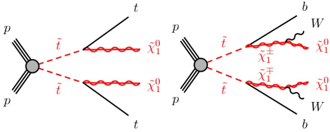
The experimental signatures of stop pair production can vary dramatically, depending on the spectrum of low-mass SUSY particles. Figure1illustrates two typical stop signatures: ˜t
1→tχ˜0
1and ˜t
1→bχ˜±
1. Other decay and production modes such as ˜t
1→tχ˜0
2and ˜t
1→tχ˜0
3, and sbottom direct pair production are also considered in the analysis. The analysis attempts to probe a broad range of the possible scenarios, taking the approach of defining dedicated search regions to target specific but representative SUSY models.
The phenomenology of each model is largely driven by the composition of its lightest supersymmetric particles, which are considered to be some combination of the electroweakinos. In practice, this means that the most important parameters of the SUSY models considered are the masses of the electroweakinos and of the colour-charged third generation sparticles.
Figure 1: Diagrams illustrating the stop decay modes, which are referred to as (left) ˜t
1→tχ˜0
1and (right) ˜t
1→bχ˜±
1. Sparticles are shown as red lines. In these diagrams, the charge-conjugate symbols are omitted for simplicity. The direct stop production begins with a top squark–antisquark pair.
In this search, the targeted signal scenarios are either simplified models [48–50], in which the masses of all sparticles are set to high values except for the few sparticles involved in the decay chain of interest, or models based on the phenomenological MSSM (pMSSM) [51, 52], in which all of the 19 pMSSM parameters are set to fixed values, except for two which are scanned. The set of models used are chosen to give a broad coverage of the possible stop decay patterns and phenomenology that can be realised in the MSSM, in order to provide as much as possible a general statement on the sensitivity of the search for direct stop production. Some of the simplified models used are designed with a goal of covering distinct phenomenologically different regions of pMSSM parameter space.
The pMSSM parametersmt Randmq3Lspecify the ˜t
Rand ˜t
Lmasses, with the smaller of the two controlling the ˜t
1 mass. In models where the ˜t
1 is primarily composed of ˜t
L, the production of light sbottoms ( ˜b
1) with a similar mass is also considered. The mass spectrum of electroweakinos and the gluino is given
by the running mass parametersM1,M2, M3, andµ, which set the masses of the bino, wino, gluino, and higgsino, respectively. If several of these parameters are comparably small, the physical LSP will be a mixed state, composed of multiple electroweakinos. Other relevant pMSSM parameters include β, which gives the ratio of vacuum expectation values (VEVs) of the up- and down-type Higgs bosons influencing the preferred decays of the stop, the SUSY breaking scale (MS) defined as MS = pmt˜
1mt˜
2, and the top-quark trilinear coupling (At). In addition, a maximal ˜t
L−t˜
Rmixing condition,Xt/MS ∼√
6 (where Xt = At − µ
tanβ), is assumed to obtain a low-mass stop (˜t
1) while maintaining the models consistent with the observed Higgs boson mass of 125 GeV [53,54].
In this search, four LSP scenarios4are considered, where each signal scenario is defined by the nature of the LSP: (a) pure bino LSP, (b) bino LSP with a light wino next-to-lightest supersymmetric particle (NLSP), (c) higgsino LSP, and (d) mixed bino/higgsino LSP, which are detailed below with the corresponding sparticle mass spectra illustrated in Figure2. Complementary searches target scenarios where the LSP is a pure wino (yielding a disappearing track signature [55] common in anomaly-mediated models [56,57]
of SUSY breaking) as well as other LSP hypotheses (such as gauge-mediated models [58–60]), which are not discussed further.
t˜1,˜b1,˜01,˜±1,˜02,˜03
t˜1,˜b1,˜01,˜±1,˜02,˜03
˜t1,˜b1,˜01,˜±1,˜02,˜03
˜t1,˜b1,˜01,˜±1,˜02,˜03 t˜1,˜b1,˜01,˜±1,˜02,˜03
˜t1,˜b1,˜01,˜±1,˜02,˜03 ˜t1,˜b1,˜01,˜±1,˜02,˜03
˜t1,˜b1,˜01,˜±1,˜02,˜03
˜t1,˜b1,˜01,˜±1,˜02,˜03 ˜t1,(˜b1)
a) pure bino LSP b) wino NLSP c) higgsino LSP d) bino/higgsino mixa) pure bino LSP b) wino NLSP c) higgsino LSP d) bino/higgsino mixa) pure bino LSP b) wino NLSP c) higgsino LSP d) bino/higgsino mixa) pure bino LSP b) wino NLSP c) higgsino LSP d) bino/higgsino mix
sparticlemasses
Figure 2: Illustration of the sparticle mass spectrum for various LSP scenarios: a) Pure bino LSP, b) wino NLSP, c) higgsino LSP, and d) bino/higgsino mix. The ˜t
1and ˜b
1, shown as black lines, decay to various electroweakino states: the bino state (red lines), wino state (blue lines), or higgsino state (green lines), possibly with the subsequent decay into the LSP. The light sbottom ( ˜b
1) is considered only for pMSSM models withmq3L<mt R.
(a) Pure bino LSP model:
A simplified model is considered for the scenario where the only light sparticles are the stop (composed mainly of ˜t
R) and the lightest neutralino. When the stop mass is greater than the sum of the top-quark and the LSP masses, the dominant decay channel is via ˜t
1 →tχ˜0
1. If this decay is kinematically disallowed, the stop can undergo a three-body decay, ˜t
1 → bWχ˜0
1 when the stop
4For the higgsino LSP scenarios, three sets of model assumptions are considered for the case of a higgsino LSP, each giving rise to different stop BRs for ˜t
1→bχ˜±
1, ˜t
1→tχ˜0
1, and ˜t
1→tχ˜0
2.
˜t1!bff0 ˜01
˜t1!bW
˜01
˜t1!t˜01 m>0
m>m˜t1 m>mW
+mb m>0
m>m˜t1 m>mW
+mb
m > 0 m > m
˜t1m > m
W+ m
bm = m
t˜1m
˜01
0 100 200 300
0 100 200 300 0 100 200 3000 100 200 300
01002003000100200300
˜ t
1! c ˜
01m>mt
m
˜t1< m
˜01m˜10 [GeV] m˜t1 [GeV]
m˜t1[GeV]m˜
0 1
[GeV]
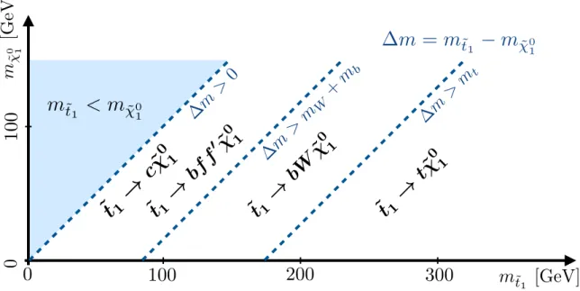
Figure 3: Illustration of the preferred stop decay modes in the plane spanned by the masses of the stop (˜t
1) and the lightest neutralino ( ˜χ0
1), where the latter is assumed to be the lightest supersymmetric particle. Stop decays to supersymmetric particles other than the lightest supersymmetric particle are not displayed.
mass is above the sum of masses of the bottom-quark,W-boson, and ˜χ0
1. Otherwise the decay proceeds via a four-body process, ˜t
1 →b f f0χ˜0
1, where f and f0are two distinct fermions, or via a flavour-changing neutral current (FCNC) process, such as the loop-suppressed ˜t
1 →cχ˜0
1. Given the very different final state, the FCNC decay is not considered further in this search. The various t˜
1decay modes in this scenario are illustrated in Figure3. The region of phase-space along the line ofmt˜
1 =m
χ˜0
1+mt is especially challenging to target because of the similarity of the stop signature to thett¯process, and is referred to in the following as the ‘diagonal region’.
(b) Wino NLSP model:
A pMSSM model is designed such that a wino-like chargino ( ˜χ±
1) and neutralino ( ˜χ0
2) are mass- degenerate, with the bino as the LSP. This scenario is motivated by models with gauge unification at the GUT scale such as the cMSSM or mSugra [61–63], whereM2is assumed to be twice as large asM1, leading to the ˜χ±
1 and ˜χ0
2having masses nearly twice as large as that of the bino-like LSP.
In this scenario, additional decay modes for the stop (composed mainly of ˜t
L) become relevant, such as the decay to a bottom-quark and the lightest chargino (˜t
1 → bχ˜±
1) or the decay to a top-quark and the second neutralino (˜t
1 → tχ˜0
2). The ˜χ±
1 and ˜χ0
2 subsequently decay to ˜χ0
1 via emission of a (potentially off-shell)W-boson or Z/Higgs (h) boson, respectively. The ˜t
1 → bχ˜±
1 decay is considered for a chargino mass above around 100 GeV since the LEP limit on the lightest chargino ismχ˜±
1
>103.5 GeV [64].
An additional ˜t
1→bχ˜±
1decay signal model (simplified model) is designed, motivated by a scenario with close-by masses of the ˜t
1and ˜χ±
1. The model considered assumes∆m(t˜
1,χ˜±
1) = 10 GeV and that the top decays via the process ˜t
1 →bχ˜±
1with a 100% BR. In this scenario the jets originating
from the bottom-quarks are too low-energy (soft) to be reconstructed and hence the signature is characterised by largeEmiss
T and no jets initiated by bottom quarks (referred to asb-jets).
(c) Higgsino LSP model:
‘Natural’ models of SUSY [23, 24, 65] suggest low-mass stops and a higgsino-like LSP. In such scenarios, the typical mass splitting (∆m) between the LSP and ˜χ±
1 varies between a few hundred MeV to several tens of GeV depending mainly on the mass relation amongst the electroweakinos.
For this analysis, a simplified model is designed for various∆m(χ˜±
1,χ˜0
1)of up to 30 GeV satisfying the mass relation as follows:
∆m(χ˜±
1,χ˜0
1)=0.5×∆m(χ˜0
2, χ˜0
1).
The stop decays into eitherbχ˜±
1,tχ˜0
1, ortχ˜0
2, followed by the ˜χ±
1 and ˜χ0
2decay through the emission of a highly off-shellW/Z boson. Hence the signature is characterised by low-momentum objects from off-shellW/Z bosons, and the analysis benefits from reconstructing low-momentum leptons (referred to as soft-leptons). The stop decay BR strongly depends on the ˜t
Rand ˜t
L composition of the stop. Stops composed mainly of ˜t
Rhave a large branching fraction to ˜t
1→bχ˜±
1, whereas stops composed mainly of ˜t
Ldecay mostly intotχ˜0
1ortχ˜0
2. In this search, both scenarios are considered separately.
(d) Bino/higgsino mix model:
The ‘Well-tempered Neutralino’ [66] scenario seeks to provide a viable dark matter candidate while simultaneously addressing the problem of naturalness by targeting a LSP that is an admixture of bino and higgsino. The mass spectrum of the electroweakinos (higgsinos and bino) is expected to be slightly compressed, with a typical mass splitting between the bino and higgsino states of 20-50 GeV. A pMSSM signal model is designed such that low fine-tuning [67,68] of the pMSSM parameters is satisfied and the annihilation rate of neutralinos is consistent with the observed dark matter relic density5(0.10<Ωh2< 0.12) [69].
The final state produced by many of the models described above is consistent with at¯t+Emiss
T final state.
Exploiting the similarity, signal models with a spin-0 mediator decaying into dark matter particles in association witht¯tare also studied assuming either a scalar (φ) or a pseudoscalar (a) mediator, where the couplings to the SM particles can be arranged by mixing with the SM Higgs (or extended Higgs) sector.
An example diagram for this process is shown in Figure4.
2.2 Analysis strategy
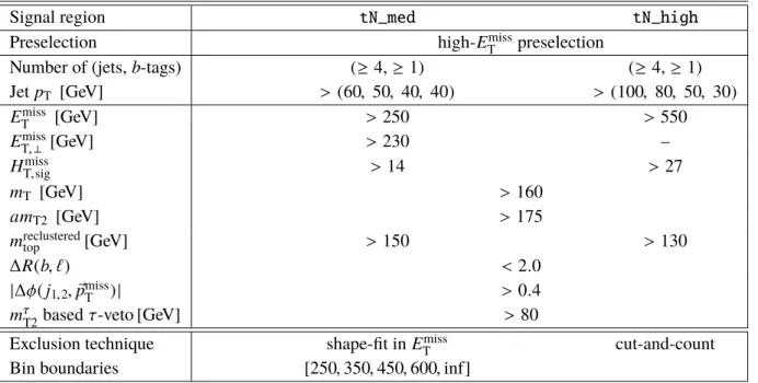
The search presented is based on 16 dedicated analyses that target the various scenarios mentioned above.
Each of these analyses corresponds to a set of event selection criteria, referred to as a signal region (SR), and is optimised to target one or more signal scenarios. Two different analysis techniques are employed in the definition of the SRs, which are referred to as ‘cut-and-count’ and ‘shape-fit’. The former is based on counting events in a single region of phase-space, while the latter employs SRs split into multiple bins in a specific discriminating kinematic variable. By utilising different signal-to-background ratios in the
5Ωandhare the density parameter and Planck constant, respectively.
φ/a
¯ t t
g g
¯ χ
χ
Figure 4: A representative Feynman diagram for s-channel spin-0 mediator production. The φ/a is the scalar/pseudoscalar mediator, which decays into a pair of dark matter (χ) particles.
various bins, the search sensitivity is enhanced in challenging scenarios where it is particularly difficult to separate signal from background. The SR selections are described in Section7.
Specialised techniques are used to enhance the sensitivity of the analyses, such as the reconstruction of hadronically decaying top-quarks from their decay products, and the use of soft-leptons for the higgsino LSP scenario. Sections5and 6describe these and other tools, chosen for their ability to discriminate signal from background. These sections are preceded by descriptions of the ATLAS detector and the dataset upon which this analysis is performed in Section3, and the corresponding set of simulated samples in Section4.
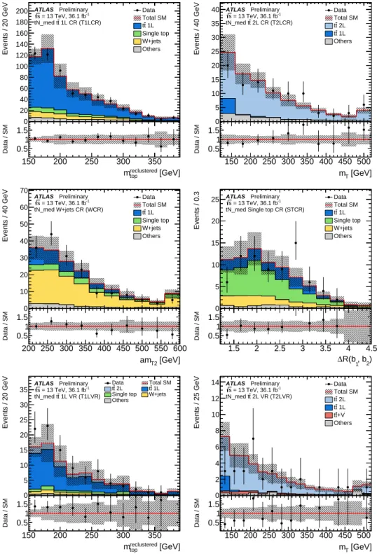
The main background processes after the signal selections includet¯t, single-topW t,t¯t+Z(→ νν)¯ , and W+jets. Each of those SM processes are estimated by building dedicated control regions (CRs) enhanced in each of the processes, making the analysis more robust against potential mis-modelling effects in simulated events and reducing the uncertainties on the background estimates. The backgrounds are then simultaneously normalised in data for each SR with its associated CRs. The background modelling as predicted by the fits is tested in a series of validation regions (VRs). The background estimation procedure, including the definition of all CRs, is detailed in Section8.
Systematic uncertainties due to theoretical and experimental effects are considered for all background and signal processes and are described in Section9. The final results and interpretations, both in terms of model-dependent exclusion limits on the masses of relevant SUSY particles and model-independent upper limits on the number of beyond-SM events, are presented in Section10.
3 The ATLAS detector and data collection
The ATLAS detector [70] is a multipurpose particle physics detector with nearly 4πcoverage in solid angle around the collision point.6 It consists of an inner tracking detector (ID), surrounded by a superconducting solenoid providing a 2 T axial magnetic field, a system of calorimeters, and a muon spectrometer (MS) incorporating three large superconducting toroid magnets. The ID provides charged-particle tracking in the range|η| < 2.5. During the LHC shutdown between Run 1 (2010–2012) and Run 2 (2015–2018), a new innermost layer of silicon pixels was added, which improves the track impact parameter resolution, vertex position resolution andb-tagging performance [71].
High-granularity electromagnetic and hadronic calorimeters cover the region |η| < 4.9. The central hadronic calorimeter is a sampling calorimeter with scintillator tiles as the active medium and steel absorbers. All the electromagnetic calorimeters, as well as the endcap and forward hadronic calorimeters, are sampling calorimeters with liquid argon as the active medium and lead, copper, or tungsten absorbers.
The MS consists of three layers of high-precision tracking chambers with coverage up to|η| = 2.7 and dedicated chambers for triggering in the region|η|< 2.4.
Events are selected by a two-level trigger system [72]: the first level is a hardware-based system and the second is a software-based system.
This analysis is based on a dataset collected in 2015 and 2016 at a collision energy of
√s = 13 TeV.
The data contain an average number of simultaneous pp interactions per bunch crossing, or “pileup”, of approximately 23.7 across the two years. After the application of beam, detector and data quality requirements, the total integrated luminosity is 36.1 fb−1 with an associated uncertainty of 3.2%. The uncertainty is derived following a methodology similar to that detailed in Ref. [73] from a preliminary calibration of the luminosity scale using a pair of x–ybeam separation scans performed in August 2015 and June 2016.
The events were primarily recorded with a trigger logic that accepts events with Emiss
T above a given threshold. To recover acceptance to signals with moderate Emiss
T , events having a well-identified lepton with a minimumpTat trigger level are also accepted for several analyses. In 2015, a Emiss
T threshold of 70 GeV at trigger level was used, while theEmiss
T threshold in 2016 was 90 GeV at the beginning of the data taking period, and raised to 100 GeV and 110 GeV for later periods. In all periods, the trigger is fully efficient for events passing an offline-reconstructedEmiss
T >230 GeV requirement, which is the minimum requirement deployed in the signal regions and control regions relying on the Emiss
T triggers. Events in which the offline reconstructed Emiss
T is measured to be less than 230 GeV are instead collected using single-lepton triggers. The thresholds for the single-lepton triggers are set to obtain a constant efficiency as a function of lepton-pTof≈90% (≈80%) for electrons (muons). In 2015, thepTthreshold was 24 GeV (20 GeV) for electrons (muons) while it was raised to 26 GeV for both electrons and muons in 2016.
6ATLAS uses a right-handed coordinate system with its origin at the nominal interaction point (IP) in the centre of the detector and thez-axis along the beam pipe. The x-axis points from the IP to the centre of the LHC ring, and the y-axis points upwards. Cylindrical coordinates(r, φ) are used in the transverse plane, φbeing the azimuthal angle around the z-axis.
The pseudorapidity is defined in terms of the polar angleθasη =−ln tan(θ/2). Angular distance is measured in units of
∆R≡
q(∆η)2+(∆φ)2.The transverse-momentum,pT, is defined with respect to the beam axis (x−yplane).
4 Simulated samples
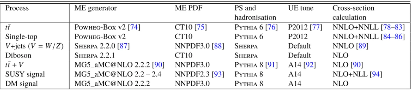
Samples of Monte Carlo (MC) simulated events are used for the description of the SM background processes and to model the signals. Details of the simulation samples used, including the matrix element (ME) generator and parton distribution function (PDF) set, the parton shower (PS) and hadronisation model, the underlying-event (UE) tune and order of the cross-section calculation, are summarised in Table1.
Table 1: Overview of the nominal simulated samples. The single-top process includest-,s-, andW tchannels.
Process ME generator ME PDF PS and UE tune Cross-section
hadronisation calculation
t¯t Powheg-Box v2 [74] CT10 [75] Pythia 6 [76] P2012 [77] NNLO+NNLL [78–83]
Single-top Powheg-Box v2 CT10 Pythia 6 P2012 NNLO+NNLL [84–86]
V+jets(V =W/Z) Sherpa 2.2.0 [87] NNPDF3.0 [88] Sherpa Default NNLO [89]
Diboson Sherpa 2.2.1 CT10 Sherpa Default NLO
t¯t+V MG5_aMC@NLO 2.2.2 [90] NNPDF3.0 Pythia 8 [91] A14 [92] NLO [90]
SUSY signal MG5_aMC@NLO 2.2 – 2.4 NNPDF2.3 [93] Pythia 8 A14 NLO+NLL [94]
DM signal MG5_aMC@NLO 2.2.2 NNPDF3.0 Pythia 8 A14 NLO
The samples produced with MG5_aMC@NLO [90] and Powheg [74, 95–98] use EvtGen v1.2.0 [99]
for the modelling ofb-hadron decays. The signal samples are all processed with a fast simulation [100], whereas all background samples are processed with the full simulation of the ATLAS detector [100]. All samples are produced with varying numbers of minimum-bias interactions overlaid on the hard-scattering event to simulate the effect of multipleppinteractions in the same or nearby bunch crossings. The number of interactions per bunch crossing is reweighted to match the distribution in data.
4.1 Background samples
The nominal t¯t sample [101] and single-top samples7 are calculated to next-to-next-to-leading order (NNLO) with the resummation of soft gluon emission at next-to-next-to-leading-logarithmic (NNLL) accuracy and are generated with Powheg interfaced to Pythia 6 for parton showering and hadronisation.
Additionaltt¯samples are generated with MG5_aMC@NLO (NLO) interfaced to Pythia8, Sherpa, and Powheg+Herwig++ [103,104] for modelling comparisons and evaluation of systematic uncertainties.
Additional samples forW W bb,W t+b, andt¯t are generated with MG5_aMC@NLO (LO) interfaced to Pythia8, in order to assess the interference effect between the singly and doubly resonant processes as a part of theW ttheoretical modelling systematic uncertainty.
Thet¯tVsamples are generated with MG5_aMC@NLO (NLO) interfaced to Pythia8 for parton showering and hadronisation. Sherpa (NLO) samples are used to evaluate the systematic uncertainties related to the modelling oft¯tV production.
7For the simulation ofW tprocess, the diagram removal (DR) scheme [102] is used.
4.2 Signal samples
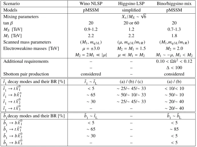
Signal SUSY samples are generated at leading-order (LO) with MG5_aMC@NLO, including up to two extra partons, and interfaced to Pythia 8 for parton showering and hadronisation. For the pMSSM models, the sparticle mass spectra are calculated using Softsusy-3.7.3 [105,106]. The output mass spectrum is then interfaced to HDECAY-3.4 [107] and SDECAY-1.5/1.5a [108] to generate decay tables for each of the sparticles. The decays of the ˜χ0
2 and ˜χ±
1 via highly off-shellW/Z bosons are computed by taking into account properly the mass of tau leptons and charm-quarks in the low∆m(χ˜±
1/χ˜0
2, χ˜0
1) regime. The details of the various simulated samples in the four LSP scenarios targeted are given below. The input parameters for the pMSSM models are summarised in Table2.
(a) Pure bino LSP:
For ˜t
1 → tχ˜0
1 samples, the stop is decayed in Pythia 8 using only phase-space considerations and not the full matrix element (ME). Since the decay products of the samples generated do not preserve the spin information, a polarisation reweighting is applied. For the ˜t
1 → bWχ˜0
1 and t˜
1→b f f0χ˜0
1samples, the stop is decayed with MadSpin [109], interfaced to Pythia 8. MadSpin emulates kinematic distributions such as the mass of thebWsystem to a good approximation without calculating the full ME. For the MadSpin samples, the stop is assumed to be composed mainly of t˜
R(∼70%), consistent with the pure bino LSP scenario.
(b) Wino NLSP:
In the wino NLSP model, the ˜t
1 is assumed to be composed mainly of ˜t
L(i.e. mq3L < mt R). The stop decays into eitherbχ˜±
1 with a branching ratio (BR) of about 66%, ortχ˜0
2with a BR of about 33%, followed by ˜χ±
1 and ˜χ0
2decays into the LSP, in a large fraction of the phase-space. Since the coupling of ˜t
Lto the wino states is larger than the one to the bino state, the stop decay to the bino state (˜t
1→tχ˜0
1) is suppressed. The BRs can be significantly different in the regions of phase-space where one of the decays is kinematically inaccessible. In the case that a mass splitting between the t˜
1and ˜χ0
2is smaller than the top-quark mass (∆m(t˜
1,χ˜0
2) < mt), for instance, the ˜t
1 →tχ˜0
2decay is suppressed, while the ˜t
1→bχ˜±
1 decay is enhanced. Similarly, the ˜t
1 →bχ˜±
1 decay is suppressed when approaching the boundary ofmt˜
1= mb+mχ˜±
1 while increasing the BR for ˜t
1→tχ˜0
1. The signal model is constructed by performing a two-dimensional scan of the pMSSM parameters M1andmq3L. For the models considered, M3=2.2 TeV andMS=1.2 TeV are assumed in order to avoid the current gluino and stop mass limits.
The decay mode of the ˜χ0
2is very sensitive to the sign ofµ, decaying into the lightest Higgs boson and the LSP (with BR∼95%) ifµ >0 and decaying into aZboson and the LSP (with BR∼75%) ifµ <0. Hence bothµscenarios are separately considered.8
Both stop and sbottom pair production modes are included. Since the stop and sbottom masses are closely related tomq3L, they have roughly the same masses. The sbottom decays largely via b˜
1→tχ˜±
1 and ˜b
1 →bχ˜0
2with a similar BR for ˜t
1→bχ˜±
1 and ˜t
1→tχ˜0
2, respectively.
8The ˜χ0
2 decay to the LSP viaZ/Higgs boson is kinematically suppressed in the off-shell regime. The ˜χ0
2 decay is instead determined by the LSP coupling to the squarks. Inmq3Lscenarios, the sbottom exchange with the large sbottom-bottom-LSP coupling contributes to the ˜χ0
2decay, resulting in the ˜χ0
2→b¯bχ˜0
1decay with a branching ratio up to 95%.
(c) Higgsino LSP:
For the higgsino LSP case, a simplified model is used with similar input parameters to the wino NLSP pMSSM model except for the electroweakino mass parameters, M1, M2, and µ, which are changed to satisfyµ M1,M2.
The stop decay BRs in scenarios withmt R < mq3Lare found to be∼50% for ˜t
1 →bχ˜±
1 and∼25%
for both ˜t
1→tχ˜0
1and ˜t
1→tχ˜0
2, independent of tanβ. On the other hand, in scenarios withmq3L <
mt R and tanβ = 20, the ˜t
1 →bχ˜±
1 BR is suppressed to∼10% while ˜t
1 →tχ˜0
1 and ˜t
1 →tχ˜0
2 are each increased to∼ 45%. A third scenario with tanβ = 60 and mq3L <mt R is also studied. In this scenario, the stop BR is found to be∼33% for each of the three decay modes. The ˜χ±
1 and ˜χ0
2
subsequently decay to the ˜χ0
1via a highly off-shellW/Z boson. The exact decay BRs of ˜χ±
1 and χ˜0
2depend on the size of the mass splitting amongst the triplet of higgsino states. For the baseline model,∆m(χ˜±
1,χ˜0
1) =5 GeV and∆m(χ˜0
2, χ˜0
1) = 10 GeV are assumed, which roughly corresponds toM1 = M2∼1.2−1.5 TeV. An additional signal model with∆m(χ˜±
1, χ˜0
1)varying between 0 and 30 GeV is considered.
In the signal generation, the stop decay BR is set to 33% for each of the three decay modes (˜t
1 →bχ˜±
1, ˜t
1→tχ˜0
2, ˜t
1 →tχ˜0
1). The polarisation and stop BRs are reweighted to match the BRs described above for each scenario. Samples were simulated down to∆m(χ˜±
1, χ˜0
1) = 2 GeV for the
∆mscan. The ˜t
1 →tχ˜0
1samples generated for the pure bino scenario are used in the region below 2 GeV, scaling by the square of BRs to the sum of ˜t
1→tχ˜0
1and ˜t
1→tχ˜0
2. (d) Bino/higgsino mix:
For the well-tempered neutralino, the signal model is built in a similar manner to the wino NLSP model. Signals are generated by scanning in M1 and mq3L parameter space, with tanβ = 20, M2= 2.0 TeV andM3 = 1.8 TeV (corresponding to a gluino mass of∼2.0 TeV).9 MS is varied in the range of 700-1300 GeV in the large ˜t
L−t˜
Rmixing regime in order for the lightest Higgs boson to have a mass consistent with the observed mass. Since the dark matter relic density is very sensitive to the mass splitting∆m(µ,M1), µis chosen to satisfy 0.10 < Ωh2 < 0.12 given the value of M1 considered (−µ∼ M1), which results in∆m(µ,M1) =20–50 GeV.
The dark matter relic density is computed using MicrOMEGAs-4.3.1f [110,111]. Softsusy-3.3.3 is used to evaluate the level of fine-tuning (∆) [67] of the pMSSM parameters. The signal models are required to satisfy a low level of fine-tuning corresponding to∆< 100 ( at most 1% fine-tuning).
For scenarios withmt R <mq3L, only stop pair production is considered while both stop and sbottom pair production are considered in scenarios withmt R >mq3L. The sbottom mass is close to the stop mass as they are both determined mainly bymq3L. The stop and sbottom decay largely into either of higgsino states, ˜χ±
1, ˜χ0
2, and ˜χ0
3with similar BRs to the higgsino models. The stop and sbottom decay BRs to the bino state are small.
Signal cross-sections for stop/sbottom pair production are calculated to next-to-leading order in the strong coupling constant, adding the resummation of soft gluon emission at next-to-leading-logarithmic accuracy
9The light sbottom and/or stop become tachyonic when their radiative corrections are large in the lowmq3Lregime, as the correction to squarks is proportional to (M3/mq3L)2, which can change the sign of the physical mass. This is an important consideration when choosing the value ofM3.