s = 13TeV pp collisiondatawiththeATLASdetector √ Searchfordirecttopsquarkpairproductioninthe3-bodydecaymodewithafinalstatecontainingonelepton,jets,andmissingtransversemomentumin ATLASCONFNote

A TLAS-CONF-2019-017 28 May 2019

ATLAS CONF Note

ATLAS-CONF-2019-017

22nd May 2019

Search for direct top squark pair production in the 3-body decay mode with a final state containing one

lepton, jets, and missing transverse momentum in √ s = 13 TeV p p collision data with the ATLAS

detector

The ATLAS Collaboration

A search for direct pair production of top squarks, the supersymmetric partner of the top quark, is presented. The search focuses on final states with one isolated electron or muon, multiple jets, and large missing transverse momentum. The analysis is performed using the Large Hadron Collider Run 2 proton-proton dataset at a centre-of-mass energy of

√ s = 13 TeV recorded by the ATLAS detector from 2015 to 2018, corresponding to an integrated luminosity of 139 fb

. One particular signal scenario is considered, characterised by the mass-splitting between the top squark and the lightest neutralino, where each top squark decays via a 3-body process to a b quark, a W boson, and a neutralino. No significant deviation from the predicted Standard Model background is observed, and limits at 95% confidence level on the supersymmetric benchmark model are set, excluding top squark masses up to 720 GeV with neutralino masses up to 580 GeV.

© 2019 CERN for the benefit of the ATLAS Collaboration.

Reproduction of this article or parts of it is allowed as specified in the CC-BY-4.0 license.

1 Introduction

Supersymmetry (SUSY) [1–9] extends the Standard Model (SM) by introducing supersymmetric partners for every SM particle, which have identical quantum numbers except for a half-unit difference in spin.

Searches for a light supersymmetric partner of the top quark, denoted as the top squark or stop, are of particular interest after the discovery of the Higgs boson [10, 11] at the Large Hadron Collider (LHC).

Top squarks may largely cancel divergent loop corrections to the Higgs-boson mass [12–19], and thus, supersymmetry may provide an elegant solution to the hierarchy problem [20–23]. The superpartners of the left- and right-handed top quarks, ˜ t

L

and ˜ t

R

, mix to form two mass eigenstates, ˜ t

1

and ˜ t

2

, where ˜ t

1

is the lighter of the two. Significant mass-splitting between the ˜ t

1

and ˜ t

2

particles is possible due to the large top-quark Yukawa coupling. A generic R -parity-conserving1 minimal supersymmetric extension of the SM (MSSM) [12, 24–27] predicts pair production of SUSY particles and the existence of a stable lightest supersymmetric particle (LSP). The mass eigenstates from the linear superposition of charged and neutral SUSY partners of the Higgs and electroweak gauge bosons (Higgsinos, winos and binos) are called charginos ˜ χ

1,2

and neutralinos ˜ χ

1,2,3,4

. In the targeted SUSY model, the lightest neutralino ( ˜ χ

1

) is assumed to be the LSP, and hence may provide a potential dark matter candidate, because it is stable and only interacts weakly with ordinary matter [28, 29].

This note presents a search for direct pair production of ˜ t

1

particles, each decaying exclusively via a 3-body process to a b quark, a W boson, and a neutralino LSP. This analysis considers the final state with exactly one isolated charged lepton (electron or muon2, henceforth referred to simply as ‘lepton’) from the decay of a W boson, high- p

jets, and a significant amount of missing transverse momentum, the magnitude of which is referred to as E

T

, from the two weakly interacting LSPs that escape detection. Dedicated searches for direct ˜ t

1

pair production were recently reported by the ATLAS [30–33] and CMS [34–40]

collaborations. The previous ATLAS and CMS searches extend the limit on the targeted model up to 600 GeV in ˜ t

1

masses at 95% confidence level.

2 Signal and search strategy

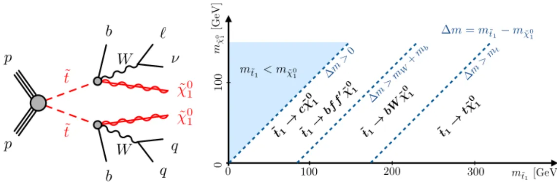
The targeted signature, referred to as ˜ t

1

→ bW χ ˜

1

is shown in the diagram in Figure 1. The signal scenario is a simplified model [41–43], in which the masses of all sparticles are set to high values except for the two sparticles involved in the decay chain of interest. Figure 1 also illustrates the kinematically allowed phase space of the stop decay, which is defined by the mass-splitting ∆m = m( t ˜

1

) − m( χ ˜

1

) . In the region where

∆m is less than the top-quark mass but larger than the sum of the b -quark and W -boson masses, the stop undergoes a 3-body decay (˜ t

1

→ bW χ ˜

1

)3. Such decays are favoured unless the mass difference is smaller than the sum of masses of the b quark and W boson, in which case the decay would proceed via a 4-body process (˜ t

1

→ b f f

χ ˜

1

). If the mass-splitting is larger than the top-quark mass, the 2-body decay mode (˜ t

1

→ t χ ˜

1

) is favoured. The search is optimised for the 3-body mode but simulated samples for the 2-body and 4-body scenarios are also considered when setting the limits.

1

A multiplicative quantum number, referred to as R -parity, is introduced in SUSY models, in order to conserve baryon and lepton number. R -parity is 1 and − 1 for all SM and SUSY particles (sparticles), respectively.

2

Electrons and muons from τ decays are included.

3

t ˜

1

also undergoes ˜ t

1

→ c χ ˜

1

when the flavour-changing neutral current (FCNC) is allowed. However, the FCNC decay is not

considered in this search.

˜ t

˜ t

W

p W p

˜ χ

b `

ν

˜ χ

b

q q

˜t¹!bff⁰˜⁰¹

˜t¹!bW

˜⁰¹

˜t¹!t˜⁰¹ m>0

m>m^˜t1 m>m^W

+m^b m>0

m>m^˜t1 m>m^W

+m^b

m >0 m > m_˜t1 m > m_W+m_b m=m˜t1 m_˜⁰

1

0 100 200 300

0 100 200 300 0 100 200 3000 100 200 300

01002003000100200300

˜t¹!c˜⁰¹

m>m^t m˜t1< m˜⁰₁

m_˜1

0[GeV] m˜t1[GeV]

m˜t1[GeV]m˜

0 1

[GeV]

Figure 1: Left: a diagram illustrating the stop decay via the 3-body mode, which is referred to as ˜ t

1

→ bW χ ˜

1

. One of the W bosons is assumed to decay leptonically. SUSY particles are shown as red lines. In this diagram, the charge-conjugate symbols are omitted for simplicity. Right: Illustration of the preferred stop decay modes in the plane ˜ t

1

- ˜ χ

1

mass plane. The neutralino is assumed to be the lightest supersymmetric particle.

In this search a set of event selections is defined, referred to as the signal region (SR), in order to discriminate between the signal and background processes. Two different analysis techniques are employed in the definition of the SR, which are referred to as ‘cut-and-count’ and ‘shape-fit’. The former is based on counting events in a single region of phase space and is used for discovery scenarios. For the latter, the SR is split into multiple bins in a discriminating variable, where the single-bin SR is a subset of the shape-fit SR. The shape-fit improves the exclusion power by utilising different signal-to-background ratios in the various bins.

The SM background after the signal selections is dominated by top quark pair production ( t¯ t ). The t¯ t background is estimated by building dedicated control regions (CRs) enhanced in the t¯ t process, making the analysis more robust against potential mis-modelling effects in simulated events as well as reducing the uncertainties in the background estimate. The background modelling as predicted by the fit is tested in a validation region (VR). The t¯ t background is then simultaneously normalised in data using a likelihood fit for the SR with its associated CR.

3 ATLAS detector and data collection

The ATLAS experiment [44] at the LHC is a multi-purpose particle detector with almost 4 π coverage in solid angle around the interaction point4. It consists of an inner tracking detector (ID) surrounded by a superconducting solenoid providing a 2 T axial magnetic field, electromagnetic, hadronic calorimeters, and a muon spectrometer (MS), which is based on three large air-core toroidal superconducting magnets. The ID provides charged-particle tracking in the range |η | < 2 . 5. During the LHC shutdown between Run 1 (2010–2012) and Run 2 (2015–2018), a new innermost layer of silicon pixels was added [45, 46], which improves the track impact parameter resolution, vertex position resolution and b -tagging performance [47].

4

ATLAS uses a right-handed coordinate system with its origin at the nominal interaction point (IP) in the centre of the detector

and the z -axis along the beam pipe. The x -axis points from the IP to the centre of the LHC ring, and the y -axis points

upwards. Cylindrical coordinates ( r, φ ) are used in the transverse plane, φ being the azimuthal angle around the z-axis. The

pseudorapidity is defined in terms of the polar angle θ as η = − ln tan ( θ / 2 ) . The transverse momentum, p

, is defined with

respect to the beam axis ( x – y plane).

High-granularity electromagnetic and hadronic calorimeters provide energy measurements up to |η| = 4 . 9.

The electromagnetic calorimeters, as well as the hadronic calorimeters in the endcap and forward regions, are sampling calorimeters with liquid argon as the active medium and lead, copper, or tungsten absorbers.

The hadronic calorimeter in the central region of the detector is a sampling calorimeter with scintillator tiles as the active medium and steel absorbers. The MS surrounds the calorimeters and is composed of three layers of precision tracking chambers with a coverage up to |η| = 2 . 7 and fast detectors for triggering in the region |η| < 2 . 4. A two-level trigger system [48] is used in order to select events. The first-level trigger is hardware-based, followed by a software-based trigger system.

The result in this note utilises the full Run 2 dataset collected from 2015 to 2018 at a centre-of-mass energy of

√ s = 13 TeV. The average number of simultaneous pp interactions per bunch crossing, referred to as “pile-up”, in the recorded dataset is approximately 34.2. After the application of beam, detector and data-quality requirements, the total integrated luminosity is 139 fb

. The uncertainty in the combined 2015–2018 integrated luminosity is 1.7%. It is derived from the calibration of the luminosity scale using x - y beam-separation scans, following a methodology similar to that detailed in [49], and using the LUCID-2 detector for the baseline luminosity measurements [50].

All events were recorded with triggers that accept events with E

T

above a given threshold. The trigger is fully efficient for events passing an offline-reconstructed E

T

> 230 GeV requirement.

4 Simulated event samples

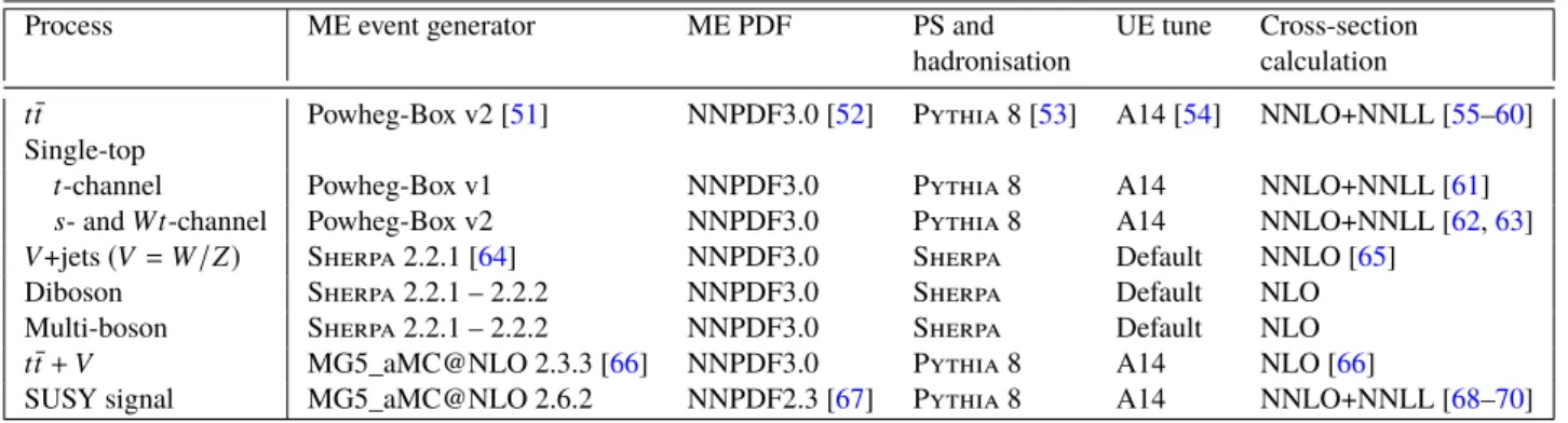
Samples of Monte Carlo (MC) simulated events are used for the description of the SM background processes and to model the signals. Details of the simulation samples used, including the matrix element (ME) event generator and parton distribution (PDF) set, the parton shower (PS) and hadronisation model, the set of tuned parameters (tune) for the underlying event (UE) and the order of the cross-section calculation, are summarised in Table 1.

Table 1: Overview of the nominal simulated samples. The cross-sections of top and V +jets background and signal samples were calculated at next-to-next-to-leading order (NNLO) with the resummation of soft gluon emission at next-to-next-to-leading-logarithm (NNLL) accuracy. The cross-sections of other background samples were calculated at next-to-leading order (NLO).

Process ME event generator ME PDF PS and UE tune Cross-section

hadronisation calculation

t t ¯ Powheg-Box v2 [51] NNPDF3.0 [52] Pythia 8 [53] A14 [54] NNLO+NNLL [55–60]

Single-top

t -channel Powheg-Box v1 NNPDF3.0 Pythia 8 A14 NNLO+NNLL [61]

s - and Wt -channel Powheg-Box v2 NNPDF3.0 Pythia 8 A14 NNLO+NNLL [62, 63]

V +jets (V = W /Z) Sherpa 2.2.1 [64] NNPDF3.0 Sherpa Default NNLO [65]

Diboson Sherpa 2.2.1 – 2.2.2 NNPDF3.0 Sherpa Default NLO

Multi-boson Sherpa 2.2.1 – 2.2.2 NNPDF3.0 Sherpa Default NLO

t t ¯ + V MG5_aMC@NLO 2.3.3 [66] NNPDF3.0 Pythia 8 A14 NLO [66]

SUSY signal MG5_aMC@NLO 2.6.2 NNPDF2.3 [67] Pythia 8 A14 NNLO+NNLL [68–70]

The samples produced with MG5_aMC@NLO [66] and Powheg-Box [51, 71–74] used EvtGen v1.6.0 [75]

for the modelling of b -hadron decays. The signal samples were all processed with a fast simulation [76],

whereas all background samples were processed with the full simulation of the ATLAS detector [76]

based on GEANT4 [77]. All samples were produced with varying numbers of minimum-bias interactions produced with Pythia 8 with the A3 tune [78] overlaid on the hard-scattering event to simulate the effect of multiple pp interactions in the same or nearby bunch crossings. The number of interactions per bunch crossing was reweighted to match the distribution in data.

4.1 Background samples

The nominal t t ¯ sample and single-top sample cross-sections were calculated at NNLO with the resummation of soft gluon emission at NNLL accuracy and were generated with Powheg-Box (at NLO accuracy) interfaced to Pythia8 for parton showering and hadronisation. Additional t t ¯ samples were generated with MG5_aMC@NLO (at NLO accuracy)+Pythia8 and Powheg-Box+Herwig7 [79, 80] for modelling comparisons and evaluation of systematic uncertainties.

W + jets and Z + jets production were generated with Sherpa v2.2.1. The production of diboson and multi-boson events was generated with Sherpa 2.2.1 – 2.2.2. The Sherpa samples used Comix [81]

and OpenLoops [82], and were merged with the Sherpa parton shower [83] using the ME+PS@NLO prescription [84]. The W + jets and Z + jets events were further normalised to the NNLO cross-sections.

The t¯ t + V samples were generated with MG5_aMC@NLO (at NLO accuracy) interfaced to Pythia8 for parton showering and hadronisation.

More details of the t¯ t , W + jets, Z + jets, diboson and t¯ t + V samples can be found in Refs. [85–88].

4.2 Signal samples

The SUSY samples were generated at leading order (LO) with MG5_aMC@NLO including up to two extra partons, and interfaced to Pythia8 for parton showering and hadronisation. The stops were decayed with MadSpin [89], interfaced with Pythia8 for the parton showering. MadSpin emulates kinematic distributions such as the mass of the bW system to a good approximation without calculating the full ME.

In order to test the sensitivity of the analysis in the adjacent 2-body and 4-body regimes, a set of ˜ t

1

→ t χ ˜

1

and ˜ t

1

→ b f f

χ ˜

1

samples were produced. For ˜ t

1

→ b f f

χ ˜

1

samples, exactly the same methodology as the ˜ t

1

→ bW χ ˜

1

was used for the production. For the ˜ t

1

→ t χ ˜

1

samples, the stop was decayed in Pythia8 using only phase space considerations and not the full ME.

The signal cross sections for stop pair production are calculated to approximate next-to-next-to-leading order in the strong coupling constant, adding the resummation of soft gluon emission at next-to-next- to-leading-logarithmic accuracy (approximate NNLO+NNLL) [70, 90–92]. The nominal cross section and the uncertainty are derived using the PDF4LHC15_mc PDF set, following the recommendations of Ref. [93].

5 Event reconstruction

Events selected in the analysis must satisfy a series of beam, detector and data-quality criteria. The primary vertex, defined as the reconstructed vertex with the highest Í

tracks

p

T

, must have at least two associated

tracks with p

> 500 MeV.

Depending on the quality and kinematic requirements imposed, reconstructed physics objects are labelled either as baseline or signal , where the latter describes a subset of the former. Baseline objects are used when classifying overlapping selected objects and to compute the missing transverse momentum. Baseline leptons (electrons and muons) are also used to impose a veto on events with more than one lepton, which suppresses background contibutions from t¯ t and Wt production where both W -bosons decay leptonically, referred to as dileptonic t¯ t or Wt events. Signal objects are used to construct kinematic and multiplicity discriminating variables needed for the event selection.

Electron candidates are reconstructed from electromagnetic calorimeter cell clusters that are matched to ID tracks. Baseline electrons are required to have p

> 4 . 5 GeV, |η | < 2 . 47, and to satisfy ‘LooseAndBLayer’

likelihood identification criteria that are defined following the methodology described in Ref. [94].

Furthermore, they must also satisfy a longitudinal impact parameter ( z

), defined as the distance from the point of closest approach between the track and the beam axis in the transverse plane to the primary vertex along the beam direction, |z

sin θ | < 0 . 5 mm. Signal electrons must pass all baseline requirements and in addition they must also have a transverse impact parameter ( d

) that satisfies |d

|/σ

< 5, where σ

is the uncertainty in d

. Furthermore, lepton isolation, defined as the sum of the transverse energy or momentum reconstructed in a cone with a certain size ∆R = p

∆η

+ ∆φ

excluding the energy of the lepton itself, is required. The isolation criteria rely on both track- and calorimeter-based information with a fixed requirement on the isolation energy divided by the electron’s p

. Photon candidates are not considered.

Muon candidates are reconstructed from combined tracks that are formed from ID and MS tracks, or stand-alone MS tracks. Baseline muons up to |η| = 2 . 7 are used, and they are required to have p

> 4 GeV and a longitudinal impact parameter | z

sin θ| < 0 . 5 mm, and to satisfy the ‘Medium’ identification criteria [95]. Signal muons must pass all baseline requirements and in addition have a transverse impact parameter |d

|/σ

< 3. Furthermore, signal muons must be isolated according to criteria similar to those used for signal electrons, but with a fixed requirement on track-based isolation energy divided by the muon’s p

.

Dedicated scale factors for the requirements of identification, impact parameters, and isolation are derived from Z → `` and J/Ψ → `` data samples for electrons and muons to correct for minor mis-modelling in the MC samples [96, 97]. The p

thresholds of signal leptons are raised to 25 GeV for electrons and muons in all signal regions.

Jet candidates are built from topological clusters [98, 99] in the calorimeters using the anti- k

algorithm [100]

with a jet radius parameter R = 0 . 4 implemented in the FastJet package [101]. Jets are corrected for contamination from pile-up using the jet area method [102–104] and are then calibrated to account for the detector response [105, 106]. Jets in data are further calibrated according to in situ measurements of the jet energy scale [106]. Baseline jets are required to have p

> 20 GeV. Signal jets must have p

> 25 GeV and |η| < 2 . 5. Furthermore, signal jets with p

< 120 GeV and |η| < 2 . 5 are required to satisfy track-based criteria designed to reject jets originating from pile-up [104]. Events containing a signal jet that does not pass specific jet quality requirements (“jet cleaning”) are vetoed from the analysis in order to suppress detector noise and non-collision backgrounds [107, 108].

Jets containing b -hadrons are identified using the MV2c10 b -tagging algorithm (and those identified are

referred to as b -tagged jets), which incorporates quantities such as the impact parameters of associated

tracks and reconstructed secondary vertices [47, 109]. The algorithm is used at a working point that

provides a 77% b -tagging efficiency in simulated t¯ t events, and corresponds to a rejection factor of about

130 for jets originating from gluons and light-flavour quarks (light jets) and about 6 for jets induced

by charm quarks. Corrections derived from data control samples are applied to account for differences between data and simulation for the efficiency and mis-tag rate of the b -tagging algorithm [109].

Jets and associated tracks are also used to identify hadronically decaying τ leptons using the ‘Loose’

identification criteria described in Refs. [106, 110], which has a 85% (75%) efficiency for reconstructing τ leptons decaying into one (three) charged pions. These τ candidates are required to have one or three associated tracks, with total electric charge opposite to that of the selected electron or muon, p

> 20 GeV, and |η | < 2 . 5. The τ candidate p

requirement is applied after a dedicated energy calibration [106, 110].

To avoid labelling the same detector signature as more than one object, an overlap removal procedure is applied. Given a set of baseline objects, the procedure checks for overlap based on either a shared track, ghost-matching [103], or a minimum distance5 ∆R between pairs of objects. First, if a baseline lepton and a baseline jet are separated by ∆R < 0 . 2, then the lepton is retained and the jet is discarded. Second, if a baseline jet and a baseline lepton are separated by ∆R < 0 . 4, then the jet is retained and the lepton is discarded, in order to minimise the contaimination of jets mis-identified as leptons. For the remainder of the note, all baseline and signal objects are those that have passed the overlap removal procedure.

The missing transverse momentum is reconstructed from the negative vector sum of the transverse momenta of baseline electrons, muons, jets, and a soft term built from high-quality tracks that are associated with the primary vertex but not with the baseline physics objects [111, 112]. Photons and hadronically decaying τ leptons are not explicitly included but enter either as jets, electrons, or via the soft term.

6 Signal selection

The SR selection is optimised using simulated event samples. The discovery sensitivity for the targeted decay mode is used as the metric of the optimisation. A signal model with a stop mass of 450 GeV and a neutralino mass of 300 GeV is chosen as benchmark and used for the SR optimisation. The benchmark is defined as a signal point that has not been ruled out in the previous search with the same final state but on the contour line of the previous limit, and hence to be targeted with larger dataset.

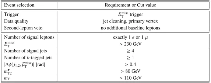
6.1 Event preselection

The event preselection depends mainly on the basic features of the decay products of the stop signal and is summarised in Table 2. All events are required to have exactly one signal lepton, no additional baseline leptons and four or more signal jets, at least one of which must be a b -tagged jet. In order to reject multijet events, a requirement is imposed on the azimuthal angles between the leading and sub-leading p

jets and E

T

( |∆φ( jet

, p ®

T

)| ). The W + jets and semi-leptonic t t ¯ background processes are largely suppressed by requiring the transverse mass6, m

, to be well above the W -boson mass. Finally, for events with hadronic τ candidates, the requirement m

T2

> 80 GeV is applied, where m

T2

[113] is a variant of the variable m

[114]. The m

T2

variable is a generalisation of the transverse mass applied to signatures

5

Rapidity ( y ≡ 1 / 2 ln (E + p

/E − p

) ) is used instead of pseudorapidity ( η ) when computing ∆R in the overlap removal procedure.

6

The transverse mass is defined as m

= q 2 p

T

E

T

[ 1 − cos (∆φ )] , where ∆φ is the azimuthal angle between the lepton and missing transverse momentum directions and p

T

is the transverse momentum of the charged lepton.

where two particles are not directly detected, and specifically targets events where a W boson decays via a hadronically decaying τ lepton.

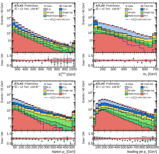
The dominant background process at preselection originates from dileptonic t¯ t production where one lepton is ‘lost’ (meaning it is either not reconstructed, not identified, or removed by the overlap removal procedure) or one W boson decays leptonically and the other via a hadronically decaying τ lepton. These t¯ t components are handled together and referred to as t¯ t 2L. Other background processes such as semi-leptonic t¯ t (referred to as t t ¯ 1L), single-top Wt , and W +jets are found to be small. Kinematic distributions at preselection are shown in Figure 2. The t¯ t background is scaled with the normalisation factor obtained from a likelihood fit in the CR, as described in Section 9, whereas the residual background contributions are normalised to the theoretical cross-sections as detailed in Section 4.

Table 2: Summary of the event preselection criteria.

Event selection Requirement or Cut value

Trigger E

T

trigger

Data quality jet cleaning, primary vertex

Second-lepton veto no additional baseline leptons

Number of signal leptons exactly 1 e or 1 µ

E

T

> 230 GeV

Number of signal jets ≥ 4

Number of b -tagged jets ≥ 1

|∆φ( j

, p ®

T

)| [rad] > 0 . 4

m

T2

> 80 GeV

m

> 110 GeV

6.2 Signal extraction with machine learning

The dominant background process after the preselection is the dileptonic t t ¯ process. In order to better discriminate the signal from the large amount of background, the SR selection is optimised by employing a machine learning (ML) approach. The ML classifier maximises the search sensitivity by learning the difference in the event topology between the signal and the t t ¯ background and by extracting correlations amongst a set of kinematic distributions being considered as input for the training.

Training and test set

In order to classify events as either signal-like or background-like in data, the ML model is trained, and its output is tested on an established mixture of signal and background events. Hence, simulated events are used to train and test the algorithm.

The size of the training sample is a crucial aspect for the performance of any ML method. Since generating

the full simulation samples with adequate sample sizes is computationally expensive, events without

detector simulation were used for the training to enhance the signal statistics by two orders of magnitude.

300 400 500 600 700 800 900 1000 [GeV]

miss

ET

0.5 1 1.5

Data / SM

[GeV]

miss

ET

1 10 102

103

104

105

Events / 40 GeV

Data Total SM

2L t

t tt 1L

W+jets Single top Multi-boson tt+V

)=(450,300) GeV 0

χ∼1 ,

~t m(

ATLAS Preliminary = 13 TeV, 139 fb-1

s

200 300 400 500 600 700 [GeV]

mT

0.5 1 1.5

Data / SM

[GeV]

mT

1 10 102

103

104

105

Events / 40 GeV

Data Total SM

2L t

t tt 1L

W+jets Single top Multi-boson tt+V

)=(450,300) GeV 0

χ∼1 ,

~t m(

ATLAS Preliminary = 13 TeV, 139 fb-1

s

50 100 150 200 250 300 350 400 450 500 [GeV]

lepton pT

0.5 1 1.5

Data / SM

[GeV]

lepton pT

1 10 102

103

104

105

Events / 25 GeV

Data Total SM

2L t

t tt 1L

W+jets Single top Multi-boson tt+V

)=(450,300) GeV 0

χ∼1 ,

~t m(

ATLAS Preliminary = 13 TeV, 139 fb-1

s

100 200 300 400 500 600 700 800 9001000 [GeV]

leading jet pT

0.5 1 1.5

Data / SM

[GeV]

leading jet pT

1 10 102

103

104

105

Events / 40 GeV

Data Total SM

2L t

t tt 1L

W+jets Single top Multi-boson tt+V

)=(450,300) GeV 0

χ∼1 ,

~t m(

ATLAS Preliminary = 13 TeV, 139 fb-1

s

Figure 2: Kinematic distributions at preselection: E

T

(top left), m

(top right), lepton p

(bottom left) and leading jet p

(bottom right). The t t ¯ background prediction is scaled by the normalisation factor obtained from a simultaneous likelihood fit of the CR (post-fit), while residual SM background processes are normalised with the respective theoretical cross-sections. The hatched area around the total SM prediction and the hatched band in the data/SM ratio include statistical and systematic uncertainties, except for the t t ¯ modeling uncertainties, which are defined only for the VR and the SR. Overflows are included in the last bin.

For the SM background processes, fully simulated and reconstructed events were used, as they contain a sufficient number of events for training the classifier.

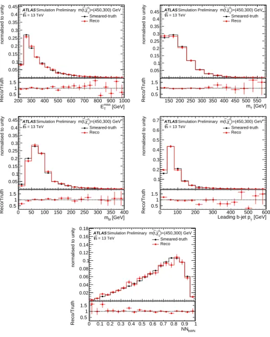
For the signal, the generated events were smeared using a dedicated procedure to emulate the effects of detector simulation and reconstruction. Parametrisations for reconstruction and identification efficiencies were obtained based on dedicated ATLAS measurements, similar to those described in Ref. [115].

Furthermore, energies or transverse momenta of selected objects at particle-level were smeared with a Gaussian term using a standard deviation corresponding to the energy (or p

) resolution of the detector.

Particle-level electrons, muons and jets were smeared according to their respective p

, η and identification working point. Additionally, flavour tagging efficiencies were applied on smeared jets. Finally, E

T

was re-computed from all smeared objects, including an approximation for the track soft term. Figure 3

shows a comparison of important kinematic distributions between smeared particle-level signal events and

fully reconstructed signal events. Similarly the same comparison for the final output score of the trained

[GeV]

miss

ET

0.05 0.1 0.15 0.2 0.25 0.3 0.35 0.4 0.45

normalised to unity

Smeared-truth Reco ATLAS Simulation Preliminary

= 13 TeV s

)=(450,300) GeV

0

χ∼1

,

~t m(

200 300 400 500 600 700 800 900 1000

[GeV]

miss

ET

0.5 1 1.5

Reco/Truth

[GeV]

mT

0.05 0.1 0.15 0.2 0.25 0.3 0.35 0.4 0.45

normalised to unity

Smeared-truth Reco ATLAS Simulation Preliminary

= 13 TeV s

)=(450,300) GeV

0

χ∼1

,

~t m(

150 200 250 300 350 400 450 500 550 [GeV]

mT

0.5 1 1.5

Reco/Truth

[GeV]

mbl

0.05 0.1 0.15 0.2 0.25 0.3 0.35 0.4 0.45

normalised to unity

Smeared-truth Reco ATLAS Simulation Preliminary

= 13 TeV s

)=(450,300) GeV

0

χ∼1

,

~t m(

0 50 100 150 200 250 300 350 400

[GeV]

mbl

0.5 1 1.5

Reco/Truth

[GeV]

Leading b-jet pT

0.1 0.2 0.3 0.4 0.5 0.6 0.7

normalised to unity

Smeared-truth Reco ATLAS Simulation Preliminary

= 13 TeV s

)=(450,300) GeV

0

χ∼1

,

~t m(

0 100 200 300 400 500 600

[GeV]

Leading b-jet pT

0.5 1 1.5

Reco/Truth

NNbWN

0.02 0.04 0.06 0.08 0.1 0.12 0.14 0.16 0.18

normalised to unity

Smeared-truth Reco ATLAS Simulation Preliminary

= 13 TeV s

)=(450,300) GeV

0

χ∼1

,

~t m(

0 0.1 0.2 0.3 0.4 0.5 0.6 0.7 0.8 0.9 1

NNbWN

0.5 1 1.5

Reco/Truth

Figure 3: Comparison of important kinematic distributions between smeared particle-level signal events (“Smeared- truth”, shown as black dots on a black histogram) and fully reconstructed signal events (“Reco” shown as red dots on a red histogram) after preselection in benchmark signal model used for the ML classifier training: E

T

(top left), m

(top right), m

(middle left), leading b -jet p

(middle right) and classifier score (bottom), referred to as NN

. Distributions are normalised to unity in order to investigate the shape of the distributions.

ML classifier, denoted NN

, is also shown in Figure 3. In general, kinematic distributions of all input variables after smearing were found to have fair agreement with the distributions at detector-level within uncertainties.

After applying the preselection on the smeared benchmark signal model, a total of approximately 200 000

signal events were selected to perform the machine learning classification, accompanied by approximately

300 000 SM background events. In order to verify the result of the training procedure, 30% of the total

signal and background statistics are reserved as a test set.

Network architecture and training

According to the kinematics of the signal model, two different types of jets are of particular importance. An energetic jet may recoil against the stop pair system, resulting in large E

T

in the final state. Additionally, low-energy jets may emerge from the decay of the stop and the subsequent hadronically decaying W boson.

Therefore, the jet multiplicity in the final states may vary significantly in the population of signal events. In order to deal with the variable length signal jet collection, the first step of the ML architecture employs a recurrent neural network (RNN). A key benefit of RNNs is the ability to extract information from sequences of arbitrary length [116]. In the second step, the output vector of the jet-based RNN is passed to a shallow neural network (NN) with two outputs corresponding to the signal and background probabilities. At this stage, additional discriminating variables are also considered and passed to the NN as input variables to improve the discriminating power of the ML classifier.

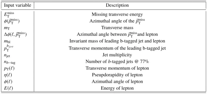
Various configurations of the ML architectures and hyperparameters were tested and optimised. The training was performed on preselected events. The RNN processes the 4-vectors of jets using the long-short term memory (LSTM) algorithm [117]. The LSTM is a specific type of RNN, capable of processing longer sequences without information loss. The LSTM transforms the variable length sequence into a 32 dimensional vector, corresponding to a maximum of 8 jets output considered. The LSTM is then connected to the input layer of a NN together with 12 additional discriminating variables. A list of the 12 input variables used to train the NN is shown in Table 3. The NN contains a single hidden layer with 128 neurons which are connected to an output neuron, representing the probability of the signal. The NN was trained using the Keras framework [118] with the TensorFlow [119] as a backend. The Adam optimiser [120] with a learning rate of 10

was used to optimise the error function. A leaky rectified linear unit (relu) [121]

with a slope coefficient of = 0 . 1 was used as activation function in the hidden layer, and a small L 2 regularisation term of λ = 10

was applied to prevent overtraining. The weight parameters corresponding to the hidden layer were initialised to a Glorot Normal distribution [122] and the training was performed in mini-batches of 32 events each, with batch normalisation [123] to accelerate the training procedure. A softmax activation function was used in the output layer to ensure that the output score of the neuron sum up to unity. Table 4 summarises the parameters of the final NN. A loss function ( cr ossentr opy ) is used to quantify the training of the signal model.

The performance of the trained ML classifier is compared to the ones of other approaches such as cut-based or other multivariate analyses in discovery significance using the metric of Z significance7, and it is found that the chosen ML classifier outperforms the other approaches in benchmark signal model by more than one standard deviation, and that removing the RNN reduces the expected significance by more than half a standard deviation.

6.3 Signal region definition

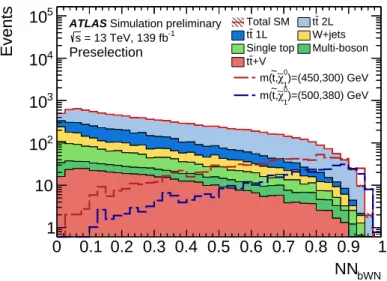
After the ML classifier is trained, the SR is defined by a stringent requirement on the classifier output score. Figure 4 shows the distribution of the classifier score, NN

. In addition to the simulated SM

7

Significance Z of observing n events for a prediction of b ± σ is defined as Z =

r

2 ( n ln [

b²+nσ²

] −

σ²

ln [ 1 +

]) when n ≥ b , or Z = −

r

2 ( n ln [

b²+nσ²

] −

σ²

ln [ 1 +

]) when n < b .

Table 3: Discriminating variables applied as inputs to the NN to train the classifier. In addition, the output vector of the jet-RNN to transform the variable length jet collection is also applied as an input to the neural network.

Input variable Description

E

T

Missing transverse energy

φ( ® p

T

) Azimuthal angle of the p ®

T

m

Transverse mass

∆φ(`, p ®

T

) Azimuthal angle between p ®

T

and lepton m

Invariant mass of leading b-tagged jet and lepton p

T

Transverse momentum of the leading b-tagged jet

n

Jet multiplicity

n

Number of b -tagged jets @ 77%

p

(`) Transverse momentum of lepton

η(`) Pseupdorapidity of lepton

φ(`) Azimuthal angle of lepton

E(`) Energy of lepton

Table 4: Architecture and hyperparameters of the neural network.

Architecture Parameter set

Number of hidden layers 1

Neurons per hidden layer 128

Activation function leaky relu ( = 0 . 1) [121]

Learning rate 10

[120]

Regularisation L 2 (λ = 10

) [116]

Weight initialisation Glorot normal [122]

Batch size 32 [116]

Batch normalisation [123] Yes

backgrounds, two signal models are overlaid to demonstrate that the ML classifier shows broad sensitivity to signal models.

The event selection for the single-bin SR as well as for the shape-fit configuration is listed in Table 5. The

shape of the NN

distribution is exploited in the shape-fit while expanding to lower bins of NN

than

the single-bin SR. For the three lowest bins in the shape-fit configuration, an additional requirement of

m

> 150 GeV is applied to suppress potential contamination from semi-leptonic t¯ t events. The dominant

background after the m

selection for the lowest three bins is dileptonic t¯ t events ( > 83 %).

0 0.1 0.2 0.3 0.4 0.5 0.6 0.7 0.8 0.9 1 NN

1 10 10

10

10

10

Events

Total SM tt 2L 1L

t

t W+jets

Single top Multi-boson +V

t t

)=(450,300) GeV

0

χ∼1

,

~t m(

)=(500,380) GeV

0

χ∼1

,

~t m(

ATLAS Simulation preliminary = 13 TeV, 139 fb-1

s

Preselection

Figure 4: Distribution of the trained ML classifier output after preselection. The t t ¯ background is not yet normalised to the CR and only statistical uncertainties are shown in the hatched shaded band.

Table 5: Overview of the signal region definition. A single-bin SR is defined for a potential data excess, while multiple bins are used to enhance the exclusion sensitivity. Square brackets indicate the interval in the NN

score. An additional requirement of m

> 150 GeV is applied to bins marked by

, in order to suppress potential contamination from semi-leptonic t t ¯ events.

Scenario SR and its binning

Discovery NN

> 0 . 9

Exclusion NN

∈ [ 0 . 65

, 0 . 7

, 0 . 75

, 0 . 8 , 0 . 82 , 0 . 84 , 0 . 86 , 0 . 88 , 0 . 9 , 0 . 92 , 1 ]

7 Background estimates

The t¯ t background process is estimated via a dedicated CR, used to normalise the simulation to the data with a simultaneous fit, discussed in Section 9. A high-purity CR is defined by relaxing the selection requirement on the output score of the ML classifier to 0 . 40 − 0 . 60. In addition, the requirement on m

is tightened to m

> 150 GeV to increase the purity of the t¯ t 2L while reducing the t t ¯ 1L contamination. The background estimate is then tested using a VR, which is disjoint from the CR and SR. The VR is defined by sliding the output score window to 0 . 60 − 0 . 65. In addition, the m

> 150 GeV requirement is kept to suppress the t¯ t 1L contamination. The background normalisation determined in the CR is applied to the VR and compared with the observed data. The boundaries of the CR and VR are carefully optimised such that the regions have a sufficient number of events that statistical uncertainties do not dominate, and that the potential signal contamination is less than 10% for signal points that are not previously ruled out by the analysis described in Ref. [30].

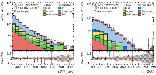
Figure 5 shows kinematic distributions in the CR and VR. Table 6 details the corresponding CR and VR

selections together with the SR selection.

300 400 500 600 700 800 900 [GeV]

miss

ET

0.5 1 1.5

Data / SM

[GeV]

miss

ET

1 10 102

103

104

Events / 40 GeV

Data Total SM

2L t

t tt 1L

W+jets Single top Multi-boson tt+V ATLAS Preliminary

= 13 TeV, 139 fb-1

s Control region

150 200 250 300 350 400 450 500 550 [GeV]

mT

0.5 1 1.5

Data / SM

[GeV]

mT

1 10 102

103

Events / 25 GeV

Data Total SM

2L t

t tt 1L

W+jets Single top Multi-boson tt+V ATLAS Preliminary

= 13 TeV, 139 fb-1

s

Validation region

Figure 5: E

T

distribution in the control region (left) and m

distribution in the validation region (right). The t¯ t process is scaled by a normalisation factor obtained in the CR. The hatched area around the total SM prediction and the hatched band in the Data/SM ratio include statistical and systematic uncertainties. The last bin contains overflows.

Table 6: Overview of the selections for the signal region and associated control and validation regions. The preselection is also applied to all regions but is not explicitly shown here. A cut of m

> 150 GeV is applied to the first three bins of the shape-fit SR as detailed in Table 5.

SR CR VR

m

[GeV] > 110 > 150 > 150

NN

> 0 . 9 ( > 0 . 65 for shape-fit) 0 . 40 − 0 . 60 0 . 60 − 0 . 65

8 Systematic uncertainties

The analysis is affected by systematic uncertainties originating from experimental effects as well as from uncertainties in the theoretical predictions and modelling. Since the yield of the t t ¯ background is normalised to data in a dedicated control region, the uncertainties on this background process are only those that affect the extrapolation from the control region into the only signal regions, and not those that change the overall normalisation. Systematic uncertainties are incorporated in the likelihood fit as nuisance parameters, which are constrained by Gaussian terms that act as a smearing factor on the expected number of events. The mean of the Gaussian is defined by the nominal prediction, while the standard deviation is determined by the size of the systematic uncertainty.

Imperfect knowledge of the jet energy scale (JES) and the jet energy resolution (JER) constitute the

dominant sources of experimental uncertainty [106, 124]. Another systematic uncertainty inherits from

measurements of the b -tagging efficiencies [125] and mis-tagging rates of c -tagged jets and light-flavour

jets [126, 127]. Variations according to the scale and resolution of the missing transverse momentum are

considered [111]. Systematic uncertainties associated with the reconstruction, identification and isolation

of electrons and muons are found to be well below 1%. Additionally, further experimental uncertainties

like the modelling of pile-up, trigger efficiencies and the estimation of the integrated luminosity have been

investigated and are found to be negligible.

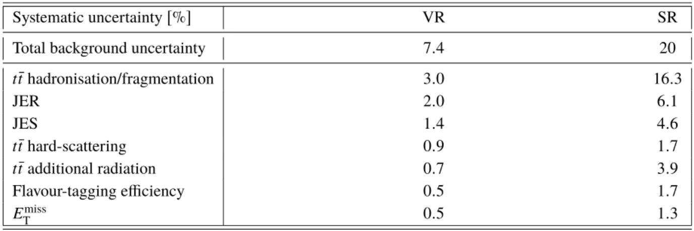
Table 7: Summary of the dominant experimental and theoretical systematic uncertainties on the total predicted SM background yield for the VR and the SR. The uncertainties are obtained using the background-only fit and are given in percentages of the total background uncertainty.

Systematic uncertainty [ % ] VR SR

Total background uncertainty 7 . 4 20

t t ¯ hadronisation/fragmentation 3 . 0 16 . 3

JER 2 . 0 6 . 1

JES 1 . 4 4 . 6

t t ¯ hard-scattering 0 . 9 1 . 7

t t ¯ additional radiation 0 . 7 3 . 9

Flavour-tagging efficiency 0 . 5 1 . 7

E

T

0 . 5 1 . 3

To evaluate the size of the systematic uncertainties on the t¯ t modelling, alternative t¯ t samples are compared to the nominal sample (Powheg-Box interfaced to Pythia8). The systematic uncertainty due to the hard-scattering process is evaluated using a comparison of the nominal t¯ t sample with a sample generated with MG5_aMC@NLO interfaced to Pythia8. Fragmentation and hadronisation uncertainties are assessed using a comparison of the nominal t t ¯ sample with a sample generated with Powheg-Box interfaced to Herwig7 [80] package for parton showering. Initial- and final-state radiation uncertainties are based on the variation of internal event weights in the nominal t¯ t sample. Variation of factorisation and renormalisation scales as well as variable shower radiation are encapsulated in the dedicated internal event weights.

The residual events from Wt , W + jets, t¯ t + V and multi-boson processes are small, with a total contribution of less than 15% in the signal regions. Theoretical uncertainties on these processes are found to have a negligible impact on the final result.

The cross section uncertainty for each signal model is taken from an envelope of cross section predictions using different PDF sets as well as factorisation and renormalisation scales, as described in Ref. [128].

Additionally, the uncertainty on the acceptance of the signal in the SR is determined from the variation of the factorisation and renormalisation scales.

In order to determine the SM background yields in the SR, a likelihood fit is performed. The background- only fit is configured to use only the CR to constrain the fit parameter corresponding to the t t ¯ normalisation.

The systematic uncertainties are obtained using the background-only fit. The contributions of the dominant systematic uncertainties are listed in Table 7 for the VR and the SR.

9 Results and interpretation

The number of observed events and the predicted number of SM background events from the background-

only fit in the VR as well as the single-bin SR are shown in Figure 6. The bottom panel shows the

significance of the observed data given the predicted SM background. The observed data agree with

the SM background prediction. Table 8 lists the number of observed events together with the predicted

number of SM background events in the SR. Moreover, the breakdown of the various backgrounds that

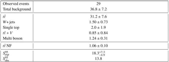
contribute to the SR is shown, as well as the result for the fit parameter that controls the normalisation of the t¯ t background (denoted the normalisation factor, NF), which is compatible with unity. The tabulated uncertainties include both statistical and systematic uncertainties. In order to quantify the level of agreement of the SM background-only hypothesis with the observed data events in the SR, a profile-likelihood-ratio test is performed. Model-independent upper limits on beyond-SM contributions are also derived for the SR.

A generic signal model is assumed that contributes only to the SR and for which neither experimental nor theoretical systematic uncertainties except for the luminosity uncertainty are considered. All limits are calculated using the CL

prescription [129].

Furthermore, the number of observed events and the predicted number of SM background events for each bin of the shape-fit SR is summarised in Table 9. Figure 7 compares the observed data and the SM background expectation in the ML classifier distribution. The bins correspond to the CR, VR, and SR.

Good agreement is found between the observed data and the SM background prediction. The bottom panel shows the significance of the observed data given the predicted SM background.

Table 8: Numbers of observed events in the single-bin SR together with the expected numbers of SM background events and their uncertainties as predicted by the background-only fit. In addition, the normalisation factor (NF) for the prediction of t t ¯ processes as obtained in the fit is listed, and the expected ( S

) and observed ( S

obs

) 95% CL upper limits on the number of beyond-SM events.

Observed events 29

Total background 36 . 8 ± 7 . 2

t t ¯ 31 . 2 ± 7 . 6

W + jets 1 . 50 ± 0 . 73

Single top 2 . 0 ± 1 . 9

t t ¯ + V 0 . 85 ± 0 . 84

Multi boson 1 . 24 ± 0 . 31

t t ¯ NF 1 . 06 ± 0 . 10

S

exp

18 . 3

S

obs

13 . 8

As no significant excess is observed, exclusion limits are set based on profile-likelihood fits for the particular top squark pair production models. The signal uncertainties and potential signal contributions to all regions are taken into account. All uncertainties except those in the theoretical signal cross-section are included in the fit. The theoretical uncertainty on the signal cross-section is evaluated and displayed separately.

Exclusion limits at 95% confidence level (CL) are obtained for each signal model and the exclusion contours are derived by interpolating in the CL

value.

Figure 8 shows the expected and observed exclusion contour as a function of stop and neutralino mass in

the targeted 3-body decay model. In addition, exclusion limits for signal points in the adjacent 2-body and

4-body regimes have been determined. The ± 1 σ

uncertainty band indicates how much the expected

limit is affected by the systematic and statistical uncertainties included in the fit. The ± 1 σ

uncertainty

lines around the observed limit illustrate the change in the observed limit as the nominal signal cross-section

is scaled up and down by the theoretical cross-section uncertainty.

0 0.5 1 1

10 102

103

104

Events

Data Total SM

t tW+jets Single top

+V t t

Multi-boson

ATLAS Preliminary

= 13 TeV, 139 fb

s

VR SR

−−20211

Significance

Figure 6: Comparison of the observed data with the predicted SM background in the VR and single-bin SR. The SM background predictions are obtained using the background-only fit configuration, and the hatched area around the total SM background prediction includes all uncertainties. The bottom panel shows the significance Z of the observed data given the predicted SM background.

Table 9: Number of observed events in each bin of the shape-fit SR together with the expected numbers of total background events and their uncertainties as predicted by the background-only fit.

Shape-fit Bin 1 Bin 2 Bin 3 Bin 4 Bin 5

NN

[ 0 . 65 , 0 . 70 ] [ 0 . 70 , 0 . 75 ] [ 0 . 75 , 0 . 80 ] [ 0 . 80 , 0 . 82 ] [ 0 . 82 , 0 . 84 ]

m

[ GeV ] m

> 150 m

> 150 m

> 150 - -

Observed events 196 215 173 61 63

Total background 238 ± 14 207 ± 17 170 ± 22 76 ± 7 63 ± 8

Shape-fit Bin 6 Bin 7 Bin 8 Bin 9 Bin 10

NN

[ 0 . 84 , 0 . 86 ] [ 0 . 86 , 0 . 88 ] [ 0 . 88 , 0 . 90 ] [ 0 . 90 , 0 . 92 ] [ 0 . 92 , 1 . 0 ]

m

[ GeV ] - - - - -

Observed events 51 42 32 16 13

Total background 54 ± 8 44 ± 7 31 ± 6 20 . 1 ± 3 . 2 17 ± 5

0.4 0.5 0.6 0.7 0.8 0.9 1 NN

− − 2 0 1 1 2

Significance

NN

10 10

10

10

10

Events

Data Total SM

t

t t t +V

W+jets Single top Multi-boson

)=(500,380) GeV

1

χ∼0 1,

~t m(

ATLAS Preliminary = 13 TeV, 139 fb

s

Figure 7: Distribution of output score of the machine learning classifier, NN

. From left to right, the bins correspond to the CR, VR and the multiple bins of the SR. The boundaries of the regions are shown as vertical dashed black lines. The SM background predictions are obtained using the background-only fit configuration, and the hatched area around the total SM background prediction includes all uncertainties. The bottom panel shows the significance Z of the observed data given the predicted SM background.

The results improve upon previous exclusion limits by excluding the stop mass region up to 720 GeV for a neutralino of about 580 GeV under the assumption of B( t ˜

1

→ bW χ ˜

1

) = 100%.

200 300 400 500 600 700 800 ) [GeV]

t 1

m( ~ 0

100 200 300 400 500 600 700 800 ) [GeV] 0 1 χ∼ m(

) > m(t)

0

χ1

∼ ) - m(

t1

~ m(

) > m(W) + m(b)

0

χ1

∼ ) - m(

t1

~ m(

) < 0

0

χ1

∼ )- m(

t1

~ m(

0

χ∼

→ t t

, ~

0

χ∼

→ bW t

, ~

0

χ∼

→ bff' t

production, ~ t

~ t

~

th

) σ

± 1 Observed limit (

exp

) σ

± 1 Expected limit ( JHEP 06 (2018) 108

ATLAS Preliminary = 13 TeV, 139 fb -1

s

Limit at 95% CL

Figure 8: Expected (black dashed) and observed (red solid) 95% excluded regions in the plane of m( ˜ χ

1

) versus m(˜ t

1

) for direct stop pair production assuming either ˜ t

1

→ t χ ˜

1

, ˜ t

1

→ bW χ ˜

1

, or ˜ t

1

→ b f f

χ ˜

1

decay with a branching ratio of 100%. The grey shaded area denotes the previously excluded regions from Ref. [30].

10 Conclusions

In this note, a search for direct top squark pair production exclusively decaying via a 3-body process to a b quark, a W boson, and a neutralino LSP is presented. The analysis targets final states with exactly one isolated electron or muon, multiple jets, and large missing transverse momentum.

The search is performed on pp collision data recorded by the ATLAS experiment at a centre-of-mass energy of

√ s = 13 TeV and corresponding to 139 fb

. The observed data are consistent with the expectation from SM processes and no significant excess is found; thus exclusion limits at 95% confidence level are derived for the considered simplified model.

In the compressed phase space, characterised by the mass splitting m(W) + m(b) ≤ ∆m( t ˜

1

, χ ˜

1

) ≤ m(t) , the result improves upon previous exclusion limits by excluding stop masses up to 720 GeV for neutralino masses up to 580 GeV, assuming a 100% decay branching ratio of ˜ t

1

→ bW χ ˜

1

.

References

[1] H. Miyazawa, Baryon Number Changing Currents , Prog. Theor. Phys. 36 (1966) 1266.

[2] R. Ramond, Dual Theory for Free Fermions , Phys. Rev. D 3 (1971) 2415.

[3] Yu. A. Golfand and E. P. Likhtman, Extension of the Algebra of Poincare Group Generators and Violation of p Invariance , JETP Lett. 13 (1971) 323, [Pisma Zh. Eksp. Teor. Fiz. 13 (1971) 452].

[4] A. Neveu and J. Schwarz, Factorizable dual model of pions , Nucl. Phys. B 31 (1971) 86.

[5] A. Neveu and J. Schwarz, Quark Model of Dual Pions , Phys. Rev. D 4 (1971) 1109.

[6] J. Gervais and B. Sakita, Field theory interpretation of supergauges in dual models , Nucl. Phys. B 34 (1971) 632.

[7] D. V. Volkov and V. P. Akulov, Is the Neutrino a Goldstone Particle? , Phys. Lett. B 46 (1973) 109.

[8] J. Wess and B. Zumino, A Lagrangian Model Invariant Under Supergauge Transformations , Phys.

Lett. B 49 (1974) 52.

[9] J. Wess and B. Zumino, Supergauge Transformations in Four-Dimensions , Nucl. Phys. B 70 (1974) 39.

[10] ATLAS Collaboration, Observation of a new particle in the search for the Standard Model Higgs boson with the ATLAS detector at the LHC , Phys. Lett. B 716 (2012) 1, arXiv: 1207 . 7214 [hep-ex] .

[11] CMS Collaboration, Observation of a new boson at a mass of 125 GeV with the CMS experiment at the LHC , Phys. Lett. B 716 (2012) 30, arXiv: 1207.7235 [hep-ex] .

[12] S. Dimopoulos and H. Georgi, Softly Broken Supersymmetry and SU(5) , Nucl. Phys. B 193 (1981) 150.

[13] E. Witten, Dynamical Breaking of Supersymmetry , Nucl. Phys. B 188 (1981) 513.

[14] M. Dine, W. Fischler and M. Srednicki, Supersymmetric Technicolor , Nucl. Phys. B 189 (1981) 575.

[15] S. Dimopoulos and S. Raby, Supercolor , Nucl. Phys. B 192 (1981) 353.

[16] N. Sakai, Naturalness in Supersymmetric Guts , Z. Phys. C 11 (1981) 153.

[17] R. Kaul and P. Majumdar, Cancellation of Quadratically Divergent Mass Corrections in Globally Supersymmetric Spontaneously Broken Gauge Theories , Nucl. Phys. B 199 (1982) 36.

[18] R. Barbieri and G. F. Giudice, Upper Bounds on Supersymmetric Particle Masses , Nucl. Phys. B 306 (1988) 63.

[19] B. de Carlos and J. A. Casas, One loop analysis of the electroweak breaking in supersymmetric models and the fine tuning problem , Phys. Lett. B 309 (1993) 320, arXiv: hep-ph/9303291 . [20] S. Weinberg, Implications of Dynamical Symmetry Breaking , Phys. Rev. D 13 (1976) 974.

[21] E. Gildener, Gauge Symmetry Hierarchies , Phys. Rev. D 14 (1976) 1667.

[22] S. Weinberg, Implications of Dynamical Symmetry Breaking: An Addendum , Phys. Rev. D 19 (1979) 1277.

[23] L. Susskind, Dynamics of Spontaneous Symmetry Breaking in the Weinberg-Salam Theory , Phys.

Rev. D 20 (1979) 2619.

[24] P. Fayet, Supersymmetry and Weak, Electromagnetic and Strong Interactions , Phys. Lett. B 64 (1976) 159.

[25] P. Fayet, Spontaneously Broken Supersymmetric Theories of Weak, Electromagnetic and Strong Interactions , Phys. Lett. B 69 (1977) 489.

[26] G. R. Farrar and P. Fayet, Phenomenology of the Production, Decay, and Detection of New Hadronic States Associated with Supersymmetry , Phys. Lett. B 76 (1978) 575.

[27] P. Fayet, Relations Between the Masses of the Superpartners of Leptons and Quarks, the Goldstino Couplings and the Neutral Currents , Phys. Lett. B 84 (1979) 416.

[28] H. Goldberg, Constraint on the Photino Mass from Cosmology , Phys. Rev. Lett. 50 (1983) 1419, Erratum: Phys. Rev. Lett. 103 (2009) 099905.

[29] J. R. Ellis, J. S. Hagelin, D. V. Nanopoulos, K. A. Olive and M. Srednicki, Supersymmetric Relics from the Big Bang , Nucl. Phys. B 238 (1984) 453.

[30] ATLAS Collaboration, Search for top-squark pair production in final states with one lepton, jets, and missing transverse momentum using 36 fb

of √

s = 13 TeV pp collision data with the ATLAS detector , JHEP 06 (2018) 108, arXiv: 1711.11520 [hep-ex] .

[31] ATLAS Collaboration, Search for a scalar partner of the top quark in the jets plus missing transverse momentum final state at √

s = 13 TeV with the ATLAS detector , JHEP 12 (2017) 085, arXiv: 1709.04183 [hep-ex] .

[32] ATLAS Collaboration, Search for direct top squark pair production in final states with two leptons in √

s = 13 TeV pp collisions with the ATLAS detector , Eur. Phys. J. C 77 (2017) 898, arXiv:

1708.03247 [hep-ex] .

[33] ATLAS Collaboration, ATLAS Run 1 searches for direct pair production of third-generation squarks at the Large Hadron Collider , Eur. Phys. J. C 75 (2015) 510, arXiv: 1506.08616 [hep-ex] . [34] CMS Collaboration, Searches for new phenomena in events with jets and high values of the M

variable, including signatures with disappearing tracks, in proton-proton collisions at √

s = 13 TeV, tech. rep. CMS-PAS-SUS-19-005, CERN, 2019, url: http://cds.cern.ch/record/2668105 . [35] CMS Collaboration, Search for direct production of supersymmetric partners of the top quark

in the all-jets final state in proton-proton collisions at √

s = 13 TeV , JHEP 10 (2017) 005, arXiv:

1707.03316 [hep-ex] .

[36] CMS Collaboration, Search for top squark pair production in pp collisions at √

s = 13 TeV using single lepton events , JHEP 10 (2017) 019, arXiv: 1706.04402 [hep-ex] .

[37] CMS Collaboration, Search for top squarks and dark matter particles in opposite-charge dilepton final states at √

s = 13 TeV , Phys. Rev. D 97 (2018) 032009, arXiv: 1711.00752 [hep-ex] . [38] CMS Collaboration, Searches for pair production of third-generation squarks in √

s = 13 TeV pp collisions , Eur. Phys. J. C 77 (2017) 327, arXiv: 1612.03877 [hep-ex] .

[39] CMS Collaboration, A search for new phenomena in pp collisions at √

s = 13 TeV in final states with missing transverse momentum and at least one jet using the α

variable , Eur. Phys. J. C 77 (2017) 294, arXiv: 1611.00338 [hep-ex] .

[40] CMS Collaboration, Inclusive search for supersymmetry using razor variables in pp collisions at

√ s = 13 TeV , Phys. Rev. D 95 (2017) 012003, arXiv: 1609.07658 [hep-ex] .

[41] J. Alwall, M.-P. Le, M. Lisanti and J. G. Wacker, Searching for Directly Decaying Gluinos at the

Tevatron , Phys. Lett. B 666 (2008) 34, arXiv: 0803.0019 .