TECHNISCHE UNIVERSIT¨AT M¨UNCHEN

Max-Planck-Institut f¨ ur Physik (Werner-Heisenberg-Institut)

Background suppression for a top quark mass measurement in the lepton+jets t t ¯ decay channel

and

Alignment of the ATLAS silicon detectors with cosmic rays

Tobias G¨ ottfert

Vollst¨ andiger Abdruck der von der Fakult¨ at f¨ ur Physik der Technischen Universit¨ at M¨ unchen zur Erlangung des akademischen Grades eines

Doktors der Naturwissenschaften (Dr. rer. nat.) genehmigten Dissertation.

Vorsitzender: Univ.-Prof. Dr. A. J. Buras Pr¨ ufer der Dissertation:

1. Hon.-Prof. Dr. S. Bethke 2. Univ.-Prof. Dr. L. Oberauer

Die Dissertation wurde am 22.12.2009 bei der Technischen Universit¨ at M¨ unchen

eingereicht und durch die Fakult¨ at f¨ ur Physik am 21.01.2010 angenommen.

Background suppression for a top quark mass measurement in the lepton+jets t t ¯ decay channel

and

Alignment of the ATLAS silicon detectors with cosmic rays

Dissertation von

Tobias G¨ ottfert

M¨ unchen

22. Dezember 2009

The investigation of top quark properties will be amongst the first measurements of ob- servables of the Standard Model of particle physics at the Large Hadron Collider. This thesis deals with the suppression of background sources contributing to the event sample used for the determination of the top quark mass. Several techniques to reduce the con- tamination of the selected sample with events from W +jets production and combinatorial background from wrong jet associations are evaluated. The usage of the jet merging scales of a k T jet algorithm as event shapes is laid out and a multivariate technique (Fisher dis- criminant) is applied to discriminate signal from physics background. Several kinematic variables are reviewed upon their capability to suppress wrong jet associations.

The second part presents the achievements on the alignment of the silicon part of the

Inner Detector of the ATLAS experiment. A well-aligned tracking detector will be crucial

for measurements that involve particle trajectories, e. g. for reliably identifying b-quark

jets. Around 700,000 tracks from cosmic ray muons are used to infer the alignment of all

silicon modules of ATLAS using the track-based local χ ² alignment algorithm. Various

additions to the method that deal with the peculiarities of alignment with cosmic rays are

developed and presented. The achieved alignment precision is evaluated and compared to

previous results.

Eine der ersten Messungen von Observablen des Standardmodells der Teilchenphysik am Large Hadron Collider wird die Untersuchung von Topquark-Eigenschaften sein. Diese Arbeit behandelt die Untergrundunterdr¨ uckung von Ereignissen, die zur verwendeten Ereignisauswahl f¨ ur die Topquark-Massenmessung beitragen. Mehrere Verfahren, um die Kontamination der ausgew¨ ahlten Ereignisse mit Ereignissen aus W +jets-Produktion und kombinatorischem Untergrund zu reduzieren, werden untersucht. Die Jet-Merging-Skalen eines k T -Algorithmus werden als topologische Variablen verwendet und multivariate Tech- niken (eine Fisher-Diskriminante) werden angewandt, um Signal von Physikuntergrund zu trennen. Weitere kinematische Variablen werden auf ihre F¨ ahigkeit zur Unterdr¨ uckung falscher Jetzuordnungen untersucht.

Der zweite Teil dieser Arbeit stellt die Fortschritte beim Alignment der Siliziummod-

ule des inneren Detektors von ATLAS vor. Ein gut alignierter Spurdetektor ist die Vo-

raussetzung f¨ ur die genaue Vermessung von Teilchenspuren, um zum Beispiel verl¨ asslich

b-Quark-induzierte Jets zu identifizieren. Etwa 700 000 Spuren aus kosmischen Myonen

werden verwendet, um die Position aller Siliziummodule von ATLAS mittels des Local-χ ² -

Alignmentalgorithmus zu bestimmen. Mehrere Erweiterungen der Methode, die sich mit

den Besonderheiten des Alignments mit kosmischen Teilchen befassen, werden eingef¨ uhrt

und pr¨ asentiert. Die erreichte Alignmentpr¨ azision wird bewertet und mit fr¨ uheren Ergeb-

nissen verglichen.

1 Introduction 1

2 Standard Model of particle physics 3

2.1 The Standard Model . . . . 3

2.1.1 Quantum chromodynamics . . . . 4

2.1.2 Electroweak interactions . . . . 4

2.2 Top quark physics . . . . 5

2.2.1 Production mechanisms . . . . 6

2.2.2 Decay processes . . . . 8

3 ATLAS at the LHC 9 3.1 The Large Hadron Collider . . . . 9

3.2 The ATLAS detector . . . . 11

3.2.1 ATLAS coordinates and terminology . . . . 12

3.2.2 Inner Detector . . . . 13

3.2.3 Calorimeter system . . . . 16

3.2.4 Muon system . . . . 17

3.2.5 Magnet system . . . . 18

4 Systematic studies for a top quark mass commissioning analysis 19 4.1 Jet reconstruction . . . . 19

4.1.1 Input objects and calibration . . . . 20

4.1.2 Jet algorithms . . . . 20

4.2 Cut-based top quark mass analysis . . . . 22

4.2.1 Object and event selection . . . . 23

4.2.2 Monte Carlo datasets . . . . 24

i

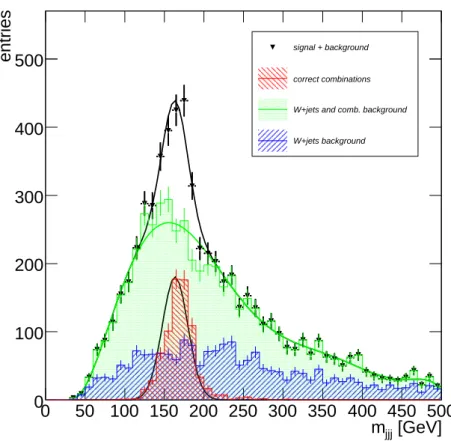
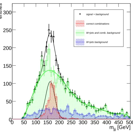
4.2.3 Mass reconstruction . . . . 26

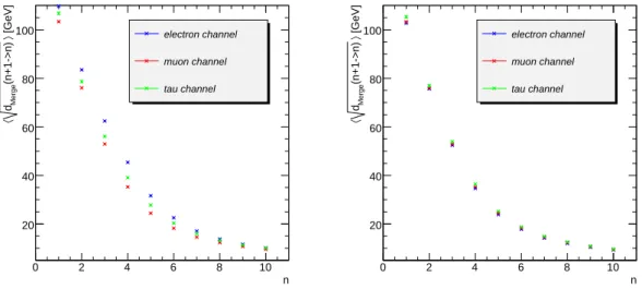
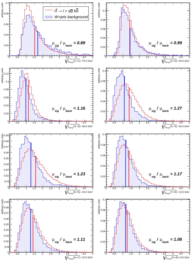
4.3 Usage of d _Merge as event shape variables for background rejection . . . . 29

4.3.1 Cut-based background rejection . . . . 30

4.3.2 Evaluation of multivariate discriminator techniques . . . . 34

4.4 Using d Merge variables to suppress wrong combinations . . . . 42

4.5 Background discrimination using kinematic variables . . . . 45

4.6 Conclusions . . . . 54

5 Alignment studies for the silicon part of the ATLAS Inner Detector 57 5.1 The local χ ² alignment algorithm . . . . 57

5.1.1 Track-based alignment . . . . 57

5.1.2 The local χ ² formalism . . . . 58

5.1.3 Tracking and the choice of residuals . . . . 59

5.1.4 Levels of alignment granularity . . . . 60

5.2 Creation of realistic systematic deformations of the ATLAS Inner Detector 61 5.3 Local χ ² alignment using cosmic ray data . . . . 67

5.3.1 Cosmic ray reconstruction and datasets . . . . 67

5.3.2 Local χ ² alignment procedure . . . . 70

5.3.3 Quality of the final alignment . . . . 98

5.4 Conclusions . . . 104

6 Conclusions 107

A Additional figures 109

B List of Abbreviations 112

List of Figures 113

List of Tables 116

Bibliography 117

Introduction

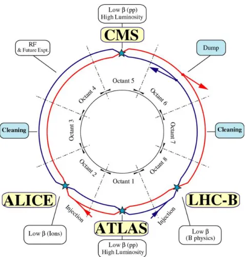
The fundamental particles and interactions that make up our universe have been investi- gated for 55 years at the European Organization for Nuclear Research (CERN) located in Geneva, Switzerland. Since then, high energy physics has reached the region of subatomic particles and provided a wealth of insight on the structure of matter and the fundamen- tal laws of nature. In a collaborative effort, the Large Hadron Collider (LHC) has been designed and built during the last 15 years to achieve an unprecedented collision energy of 14 TeV in its proton-proton collisions. Four main experiments were constructed, which aim to allow for physics analyses that test the Standard Model of particle physics and explore the regions where it is no longer valid. One of these experiments is ATLAS (A Toroidal Lhc ApparatuS).

After the successful beam injection in September 2008 and the following cryogenic incident, the accelerator and the experiments were preparing for a restart this autumn.

The major points of work for ATLAS are the successful commissioning of all detector systems to take advantage of, and understand as much as possible, the performance of the experiment, and the preparation of physics analyses to be used for the early data that is now being recorded after the LHC restart.

Top-antitop quark pair production will already set in with a high rate at the early stages of proton-proton collisions. Top quark production and decay is an important topic, since it allows to test the Standard Model to high precision and additionally it appears as background process to many searches for physics beyond the Standard Model.

For a better reduction of backgrounds to top quark decay, the identification of b quark induced jets is of high importance, which can only be achieved with a well-commissioned tracking detector. The alignment of the ATLAS Inner Detector prior to proton-proton col- lisions is performed using muons which originate from interactions of cosmic ray particles with the atmosphere and that traverse the detector. Track-based alignment methods then can determine the positions in space of all modules to enable decent vertex and tracking resolution. Later, the Inner Detector measurements will be refined to their full resolution by alignment with tracks from proton-proton collisions.

This thesis is structured into the following chapters:

• Chapter 2 briefly reviews the Standard Model of particle physics and the properties of top quark production and decay.

1

• Chapter 3 introduces the ATLAS detector. The detector design and its physics requirements are illustrated and the individual subdetectors are described.

• Chapter 4 covers the results from systematic investigations on the main backgrounds for top quark mass reconstruction. The cut-based commissioning analysis that de- termines the top quark mass from the lepton+jets decay channel of top quark pair production is introduced. This is a robust analysis that only relies on basic func- tioning of the detector components and does not use b-quark identification. Event shape variables using the k T jet algorithm are investigated upon their discrimination against background arising from W +jets physics processes and wrong jet association.

A multivariate technique (Fisher discriminant) is introduced and its performance is evaluated. Several other kinematic variables are explored to improve the rejection of W +jets and combinatorial background.

• Chapter 5 presents the results on the alignment of the ATLAS silicon modules within the Inner Detector using cosmic muon data taken in 2008. The local χ ² alignment algorithm is described and applied to data, together with the improvements that have been made to the software within this thesis. A study on creation of semi-realistic systematic deformations of the Inner Detector is presented. These deformations are used to test the alignment and physics performance of the ATLAS software.

• Chapter 6 presents the summary and conclusions of the thesis, with the important

results highlighted and an outlook to further developments given.

Standard Model of particle physics

2.1 The Standard Model

The Standard Model of particle physics [1] is a set of relativistic quantum field theories.

It is at present the most precise description of elementary particle physics at the micro- scopic scale. It encompasses quantum chromodynamics (QCD) and electroweak theory with quantum electrodynamics (QED) and weak interactions. All components fulfil the requirements of being renormalisable, i. e. their divergences can be cancelled and they yield finite results for the physical observables. They are gauge invariant, meaning there are local gauge symmetries that make it possible to choose certain parameters without changing the dynamics of the theory. The total symmetry group of the Standard Model is the SU (3)⊗ SU (2) ⊗U (1) group, which describes the symmetries of QCD and electroweak theory.

The particle content of the Standard Model is as follows: the fermions of spin 1/2 form the matter particles, whereas the spin 1 bosons are the exchange quanta of the force fields. In the fermion sector, there are six quark flavours, namely up, down, charm, strange, top, and bottom (u, d, c, s, t, b) quarks, which make three generations (or families) of doublets. Each of the quarks appears in three versions with different colour charge in addition to their electroweak charge. The three generations of leptons, namely, electron (e), muon (µ) and tauon (τ ), together with their respective neutrinos, have no colour charge but electroweak charges. The force carrier particles are the massless photons (γ ), the massive weak interaction gauge bosons W ^± and Z, and the eight massless gluons (g) that mediate the strong force. In addition, the favoured mechanism for breaking the electroweak symmetry necessitates that there exists at least one spin 0 boson, the Higgs boson (H), which is the only elementary particle of the Standard Model not yet observed. The fourth elementary force known, gravity, has negligible influence at the microscopic scale and is not included in the Standard Model.

All experimental data up to energies of a few hundred GeV strongly support the Standard Model calculations and make it one of the best-tested theories in physics up to now. However, several areas of the theory indicate that it cannot be valid up to energies higher than a few TeV and therefore strongly motivate the search for physics and theories beyond the Standard Model. Amongst the most promising candidates are supersymmetry, theories with extra dimensions and string theory, that strive for solving some or all of the

3

problems of the Standard Model. To observe phenomena predicted by these models, a firm understanding of the Standard Model is needed.

2.1.1 Quantum chromodynamics

QCD [2, 3] is the part of the Standard Model describing strong interactions. It is based on the symmetry group SU (3) with six different quark flavours being colour triplets and eight gluon fields (together called partons). Leptons and the gauge bosons of electroweak theory do not carry colour charges and thus do not participate in strong interactions.

Unlike the photon in QED, gluons carry colour charges themselves, allowing for self- coupling in 3-gluon and 4-gluon vertices. Therefore QCD is a non-Abelian theory, meaning that the generators of the algebra do not commute. Other striking features of QCD are confinement and asymptotic freedom, i. e. the impossibility of observing free quarks outside of bound hadron states and the asymptotic vanishing of the coupling for interactions with high momentum transfer (deep inelastic processes). The QCD coupling α _s varies as a function of the four momentum transfer Q, as given by (in next-to-leading order, NLO):

α s (Q ² ) = α s (µ ² ) 1 + α s (µ ² )β 0 ln ^Q _µ

. (2.1)

This equation gives the evolution of α _s from a known scale µ ² to a different scale Q ² , with β 0 > 0 being the first term in the expansion of the β-function of the renormalisation group equation. It can be seen that for growing Q ² , α _s asymptotically vanishes, which describes the asymptotic freedom. For small Q ² , α _s eventually diverges, and the region of confinement is reached, where perturbative expansions cannot be done anymore. The current knowledge of α _s at the Z mass is α _s (M _Z

) = 0.1184 ± 0.0007 [4].

Confinement also results in the observation of jets in hadron collisions, which are narrow streams of hadronic particles created in hard parton collisions. Jets arise due to the creation of new colourless quark-antiquark pairs from the vacuum when trying to separate bound quarks in a hard interaction.

2.1.2 Electroweak interactions

Electroweak theory [5–8] unifies weak interactions and electromagnetism. Its Lagrangian

obeys the gauge group SU (2) ⊗ U (1). It is a chiral theory in the sense that it affects

right-handed and left-handed fields differently. All right-handed fermionic fields are elec-

troweak singlets, whereas the left-handed fields are doublets. This forbids mass terms for

the fermions, and they are reintroduced into the Standard Model together with W ^± and

Z masses by the mechanism of electroweak symmetry breaking. The standard way to intro-

duce the symmetry breaking is via the Higgs mechanism [9]. It does so by spontaneously

breaking the symmetry group via a doublet of complex scalar fields Φ with a non-vanishing

vacuum expectation value (v ≈ 246 GeV). Three of the four degrees of freedom of Φ are

absorbed into the longitudinal degree of freedom of massive spin-1 bosons (of the W ^± and

Z), while the photon stays massless. The remaining degree of freedom is physical and

should be found as the Higgs boson. A huge experimental effort is undertaken to find this

last missing piece in the Standard Model, especially at the various LHC experiments.

Weak interactions are the only Standard Model interactions that change flavour. The weak eigenstates of the fermions, where W bosons couple to, are not the eigenstates of the freely propagating particles, the mass eigenstates. The mixing of the down-type quark mass eigenstates into the weak eigenstates is parameterised in the 3×3 Cabibbo-Kobayashi- Maskawa (CKM) matrix [10, 11]. The mixing of the neutrino mass eigenstates into their weak eigenstates is parameterised in the 3×3 Pontecorvo-Maki-Nakagawa-Sakata (PMNS) matrix [12, 13]. The weak and mass eigenstates for up-type quarks and charged leptons are chosen to be identical.

2.2 Top quark physics

The top quark plays an important role in high energy physics [14]. It is by far the heaviest observed elementary particle. The discovery of its existence was made in 1995 by the CDF and D0 collaborations [15, 16] at the TeVatron collider at Fermilab. The current combined measurements of the two detectors [17] result in a top quark mass of 173.1 ± 1.3 GeV ¹ .

The top quark carries a number of interesting properties, which make it special amongst the Standard Model quarks:

• Due to its short lifetime, the top quark is the only quark that decays as a bare quark, i.e. before it can form bound states. The top decay width at NLO is calculable to be Γ t = 1.36 GeV [18]. This corresponds to a lifetime of about 0.5 · 10 ⁻²⁴ s, which is too short to observe bound states involving top quarks. This is also not enough time for chromomagnetic spin depolarisation, and the top quark passes on its spin to its decay particles.

• The Yukawa coupling of the top quark, i. e. the coupling to the Higgs boson, as given by √

2m t /v, is almost unity, which is already interesting on its own. Since the top quark has the largest Yukawa coupling of all quarks, it will play an important role in understanding the mechanism of electroweak symmetry breaking.

• Quantum electroweak theory links the mass of the Higgs boson with the masses of the W boson and the top quark via virtual loop corrections. This gives the possibility to constrain the Higgs boson mass by measuring the two other masses at high precision.

Some properties of the top quark are already known quite precisely, most notably the mass, while many others are still unmeasured or only known vaguely. For example, the electric charge of the top quark has not yet been measured, which leaves the possibility that the observed particle is in fact some exotic type of quark having an electric charge other than 2/3. Recent analyses however exclude this scenario at 92 % CL [19]. At the LHC, the charge of the top quark can be measured with an expected precision of O(10 %) [14].

Finally, a good understanding of top quark properties and production and decay mech- anisms is also essential for other physics at the ATLAS detector: top quark production and decay processes can serve as important data to calibrate and commission the detector.

Moreover, almost all analyses that search for physics beyond the Standard Model have to cope with top quark production and decay as background processes.

1

For the whole of this thesis natural units will be used, i. e. ¯ h = c = 1

t

q t q

t t t

t t

t

+ +

g

g g

g g

g

Figure 2.1: The lowest-order Feynman diagrams contributing to t ¯ t production. These are q q-annihilation (upper) and gluon-gluon-fusion (lower). ¯

2.2.1 Production mechanisms

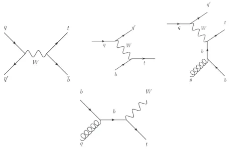
The production mechanisms of top quarks at hadron colliders are twofold: There are top-antitop pair production and single top quark production mechanisms. The Feynman diagrams contributing to t t ¯ production at lowest order are shown in figure 2.1. These are q q-annihilation and gluon-gluon-fusion. The Feynman diagrams contributing to single top ¯ quark production at lowest order are shown in figure 2.2. These are s-channel production, two t-channel processes and the associated production of a top quark with a W boson.

The cross sections for these processes can be calculated by factorizing them into the hard scattering process of the two partons and the parton longitudinal momentum distribu- tion functions (PDFs) in the incoming protons. The matrix element of the parton-parton interaction can be calculated and is denoted with ˆ σ ^i,j for two partons of type i and j. The PDFs f i (x i , µ ² _F ) are not calculable from the theory, but rather are the results of parame- terised fits to data from deep-inelastic scattering and other experiments. The total cross section for top quark pair production is then given by

σ _t t ¯ ( √

s, m ² _t , µ ² _r , µ ² _F ) = X

i,j=q,¯ q,g

Z

dx _i dx _j f _i (x _i , µ ² _F )f _j (x _j , µ ² _F )·ˆ σ ^{ij→t ¯ t} ( √

s, m ² _t , x _i , x _j , µ ² _r , µ ² _F ) , (2.2) where √

s denotes the centre-of-mass energy of the partonic collision, x i and x j are the momentum fractions of the respective protons that the partons i and j carry. The symbol µ _r denotes the renormalisation scale at which the matrix element calculation is performed, and µ F is the factorisation scale at which the parton density functions are evaluated. A usual choice is to set µ _r = µ _F = m _t .

Single top quark production is calculated to have about 50 % of the cross section of top quark pair production. A comparison of calculated production cross sections at LHC energies is given in table 2.1. From the cross sections one can see that at an integrated luminosity of 100 fb ⁻¹ , which is the design luminosity per year expected for the LHC experiments, top quarks will be produced in high abundance (about 100 million pairs).

This means that every measurement of top quark properties will soon be dominated by

systematic uncertainties.

t

q

b q

W

q

b q^′

t

q

q^′

W

W

g

t

b

b

W

q t b

b

Figure 2.2: The lowest-order Feynman diagrams contributing to single top quark produc- tion. These are s-channel (upper left), t-channel (upper middle and right) and Wt-channel (lower).

Table 2.1: Calculated production cross sections for top quark single and pair production at various LHC energies. The t ¯ t calculations are done in approximate NNLO with the PDF parametrisation CTEQ6.6 and an assumed top quark mass of m t = 172.5 GeV [20]. For the single top quark processes at √

s = 10 TeV, the program MCFM was used to calculate the cross sections to NLO using a top quark mass of m _t = 172.5 GeV [21]. The single top quark cross sections at √

s = 14 TeV are calculated to NLO for the s- and t-channel [22]

and for the W t-channel [21], assuming m t = 175 GeV. These cross sections are also used as reference for the ATLAS Monte Carlo production of top quark samples.

top quark pair production

√ s σ _t ¯ t

10 TeV 401.60 pb

14 TeV 883.90 pb

single top quark production

√ s σ s−channel σ t−channel σ W t−channel

10 TeV 6.627 pb 124.51 pb 32.66 pb

14 TeV 10.65 pb 246.6 pb 66 pb

After the discovery of top quark pair production in 1995, single top quark production was also discovered recently at the TeVatron detectors [23, 24].

2.2.2 Decay processes

The top quark decays almost exclusively to a W boson and a b quark, as reflected by the large V tb matrix element in the CKM matrix of almost unity. The current best estimates of the CKM matrix elements involving top quarks, imposing the unitarity of the matrix, are given in the following [18]. These lead to the predicted branching fractions Br(t → W q) that favour t → W b over all other decays:

|V _td | = 0.0087 ^{+3.0 %} _{−4.2 %} ⇒ Br(t → W d) ≈ 0.01%

|V _ts | = 0.0407 ± 2.5 % ⇒ Br(t → W s) ≈ 0.17%

|V _tb | = 0.9991 ± 0.004 % ⇒ Br(t → W b) ≈ 99.82%

The W boson then further decays either leptonically into eν e , µν µ or τ ν τ or hadron- ically into q q ¯ ⁰ with q = u, d, s, c. This leaves three main decay channels for t t ¯ pairs, characterised by the number of leptons and jets they produce. They are called di-lepton channel (ll), all-hadronic channel, and lepton+jets channel (l+jets), and their respective branching fractions are given in table 2.2.

Table 2.2: The expected branching fractions for the various decay channels of top quark pairs, calculated from the measured W decay fractions [18]. In this table, ˆ l stands for e, µ.

decay mode Br

di-lepton t ¯ t → ˆ lν _{ˆ l} b ˆ l ⁰ ν _{ˆ l}

b 4.5%

t ¯ t → ˆ lν _{ˆ l} bτ ν _τ b 4.8%

t ¯ t → τ ν _τ bτ ⁰ ν _τ

b 1.3%

all-hadronic t ¯ t → qq ⁰ bq ⁰⁰ q ⁰⁰⁰ b 45.7%

lepton+jets t ¯ t → ˆ lν ˆ l bqq ⁰ b 28.8%

t ¯ t → τ ν τ bqq ⁰ b 15.2%

The analysis described in this thesis focuses on the l+jets channel, since this chan- nel offers a good compromise between high branching fraction and good experimental reconstruction properties. The ll channel only offers 10.6 % of all decays, while possess- ing the additional complication of two neutrinos in the final state. This makes kinematic reconstruction of the decay products ambiguous. The all-hadronic channel offers 45.7 % branching fraction, while making it necessary to correctly assign the six jets in the final state to the two decaying top quarks. This leaves at least 10 combinations per event to consider (assuming no b-tagging). The l+jets channel possesses 44.0 % branching fraction and has only one neutrino in the final state. The leptonically decaying top quark can be used for tagging the event.The mass of the top quark can then be extracted from a full re- construction of the hadronically decaying top. Since τ leptons are hard to reconstruct, one often restricts the analysis to electrons and muons for leptonically decaying top quarks.

In this case, the l+jets channel still offers a branching fraction of 28.8 %.

ATLAS at the LHC

3.1 The Large Hadron Collider

The Large Hadron Collider [25] is the large proton-proton ring collider located at the CERN site. It is designed to deliver unprecedented collision energy and luminosity to the four main experiments: ALICE [26], CMS [27], LHCb [28] and ATLAS [29]. The design centre-of-mass energy of the LHC is √

s =14 TeV with two beams of 7 TeV protons colliding. After the magnet accident in September 2008 [30], it was decided that the LHC will initially operate at 3.5 TeV proton energy at the startup in autumn 2009. This lowers the demands on the magnetic field strengths of the dipole magnets, of which not all are commissioned to the final 7 TeV proton energy yet.

The event rate for a given process is directly proportional to the luminosity of the machine and the cross section of the process:

N = L σ( √

s) . (3.1)

The luminosity depends only on machine parameters and can be calculated in the assump- tion of Gaussian beam profiles as:

L = f n ² 4πσ x σ y

, (3.2)

with f being the collision frequency, n the number of protons per bunch and σ _x , σ _y the transverse beam widths.

At the design luminosity of L = 10 ³⁴ cm ⁻² s ⁻¹ , the LHC ring will contain 2 ×2808 pro- ton bunches with 11.5 · 10 ¹⁰ protons per bunch at a collision frequency of f = 40 MHz.

During the startup phase, the luminosity will be considerably lower, in the range of (10 ³⁰ − 10 ³² ) cm ⁻² s ⁻¹ . The expected integrated luminosity within the first year of LHC running is around 100 pb ⁻¹ . The startup phase will be followed by a low-luminosity phase, which will provide L ≈ 10 ³³ cm ⁻² s ⁻¹ . In this phase, one can expect around 10 fb ⁻¹ per year. Finally, the design luminosity will deliver 100 fb ⁻¹ annually.

The LHC can also accelerate heavy ions. It is planned to have lead-lead collision runs with up to L = 10 ²⁷ cm ⁻² s ⁻¹ , which will be investigated mainly by ALICE, but also by the other experiments.

A sketch of the LHC ring with the interaction points can be seen in figure 3.1.

9

Figure 3.1: A sketch of the LHC ring with the different collision points and the experiments.

3.2 The ATLAS detector

The ATLAS detector [29] is one of the two big multi-purpose detectors for the LHC particle collisions. Its design has to fulfil several conditions to make optimal use of the physics potential that the LHC accelerator offers. Amongst the primary requirements are:

• a radiation hard design, especially for the Inner Detector, and the ability to cope with the high occupancies and trigger rates when operated at the high luminosity and bunch crossing rate that the LHC delivers,

• an acceptance as close as possible to a full 4π solid angle to detect all collision products, even when the centre-of-mass system of the hard interaction is highly boosted, and to reliably deduce missing transverse energy,

• very good momentum resolution and secondary vertex determination in the Inner Detector for a precise track reconstruction and a good b-quark tagging efficiency,

• calorimeters with very good energy resolution and coverage plus small energy leakage to measure jets and missing energy precisely,

• a good identification and momentum resolution for electrons and muons and the ability to identify the sign of charge for very high momentum particles,

• a fast and efficient trigger system to get good sensitivity for many of the interesting physics processes.

In order to fulfil all these requirements, the following overall design has been chosen, which will be described in more detail in the following sections:

• an Inner Detector comprising three subsystems with different technologies:

– The Pixel detector employs radiation hard silicon pixel sensors to reach high granularity and good vertex resolution around the interaction point.

– The SemiConductor Tracker (SCT) employs silicon strip sensors in double lay- ered modules to provide precise spacepoint measurements of the tracks outside the Pixel detector volume.

– The Transition Radiation Tracker (TRT) as the outermost of the three uses many layers of kapton tubes with gold wires, interspersed with plastic foils and fibres. It is designed to provide high momentum resolution. In addition, particle identification via the detection of transition radiation photons is made possible.

• a calorimeter system with high-granularity sampling calorimeters made of different absorbers and active materials

• a muon system extending to large radii within a toroidal magnetic field

• a magnet system with two different orientations for the magnetic field:

– a superconducting solenoidal magnet enclosing the Inner Detector and produc-

ing a field of about 2 T

Figure 3.2: Computer generated sketch of ATLAS with its subsystems and dimensions labelled [31].

– eight superconducting large toroidal coils with air core technology comple- mented by two endcap toroidal coils providing bending power within the huge volume of the muon system.

Figure 3.2 shows a computer generated sketch of ATLAS with the different subsystems indicated. The persons on the figure give an impression of the large size of the detector.

3.2.1 ATLAS coordinates and terminology

Throughout this thesis, the following sets of coordinates will be used:

• The ATLAS global coordinate system is a right-handed orthogonal system, where the Z -axis follows the beamline and the X-Y -plane is perpendicular to it. The X-axis is defined to point towards the centre of the LHC ring, the Y -axis points upwards.

The side of the detector with positive Z is defined to contain endcap A; endcap C lies in the negative Z side.

• Often cylindrical coordinates are used, which have the form (R, φ, θ), where R is the distance from the Z -axis, φ is the azimuthal angle and θ the polar angle measured from the positive Z -axis. The pseudorapidity η is defined as η = − ln tan(θ/2).

Distances in angular space are usually given in terms of ∆R = p

∆φ ² + ∆η ² , which

is invariant under Lorentz boosts along the Z-axis.

Figure 3.3: A computer generated sketch of the ATLAS Inner detector [31].

• Every detector element within ATLAS has a per-module local coordinate system, which is also righthanded and orthogonal. These coordinates will be denoted with (x, y, z). Additionally, for alignment rotations around these axes will frequently be determined. The rotations around the local x, y, z axes are called α, β, γ, respectively.

3.2.2 Inner Detector

The Inner Detector is used to accurately reconstruct tracks of charged particles and their momenta and charge sign, as well as the primary and possible secondary vertices in the collision. A sketch of the three subsystems can be seen in figure 3.3. They are described in the following, starting from the inside:

Pixel detector

The Pixel detector consists of 1744 rectangular modules of size 19×63 mm ² , of which 1456 are located in the three barrel layers and 2 × 144 in the 2 × 3 endcap disks. The pixel detector dimensions are 1.3 m in length and 150 mm in radius, with the innermost layer at a radius of 50.5 mm away from the beamline.

The barrel is composed of staves of pixel modules, where 13 modules are mounted onto a support structure. The middle module lies parallel to the beamline, whereas the other modules are shingled slightly to create overlaps in the Z direction. The staves are mounted as bi-staves with a common cooling unit to the barrel such that the modules are inclined by 20 ^◦ with respect to the tangent of the layer in the R-Φ plane (turbine arrangement).

This creates overlap and therefore full coverage in R-Φ and compensates for the mean of

the Lorentz drift angle in the magnetic field of the Inner Detector. The endcaps possess

one ring of pixel modules each, where the modules are parallel to the R-Φ plane and to

each other and overlap by alternating frontside and backside mounting on the support disk.

All pixel modules are identical and possess 47232 rectangular pixels with the usual size of 50 × 400 µm ² . They are read out by 16 front-end (FE) chips in two rows and eight columns, which need a small gap between each other. Thus, 4 pixels in each FE chip column are ganged together, i. e. are read out by the same channel on the FE chip. This leads to 46080 readout channels in total on a pixel module. The sensor is made of 250 µm thick n ⁺ -in-n silicon, where the pixels are bump-bonded to the respective readout channels of the FE chips.

The use of highly oxygenated silicon and the n ⁺ -in-n design allow the pixel modules to be operated at the very high radiation fluences close to the beam. To slow down the radiation damage and control the leakage currents, the pixel detector will be operated at a temperature of −5 ^◦ C to −10 ^◦ C. The n-type silicon bulk will type-invert into p-type material after a fluence of Φ _eq (1 MeV neutron equivalent) ≈ 2·10 ¹³ cm ⁻² ; from then on the depletion zone will grow starting from the n ⁺ pixel implants and maintain a good charge collection efficiency at low bias voltages. However, the performance of the innermost pixel layer is expected to strongly deteriorate after roughly three years of running at design luminosity.

The pixel detector delivers three space points per track and is the most important detector for a precise vertex, secondary vertex and pileup vertices determination. The design goals put stringent requirements on the spatial resolution and thus the allowed alignment tolerances, which can eventually only be reached by track-based alignment.

The required precisions are listed in table 3.1. They are derived from the demand that the detector misalignment must not reduce the track parameter resolutions by more than 20 % [32]. In addition, the estimated as-built accuracy as well as the intrinsic resolution of the sensors are listed. The high as-built accuracy for pixel endcap modules comes from a precise survey of the assembled endcap disks. However, it only measures relative module- to-module positions and not absolute positions in space so that a precise alignment is still needed. The other as-built precisions stem from the mounting precisions of the modules on the support structures and (much smaller) the module fabrication tolerances. These numbers can only give estimates of the positioning precision, since the module locations might well change by assembling the individual subdetectors to the full Inner Detector, lowering them into the experimental cavern and cooling the detector to its operating temperature.

The local coordinate system for every pixel module is as follows: The origin of the coordinate system is in the centre of the rectangular module, the x-coordinate runs along the short side of the pixels, the y-coordinate runs along the long side of the pixels. The local z-coordinate is normal to the plane of the module and pointing away from the interaction point.

SemiConductor Tracker

The SCT consists of 4088 modules with single-sided silicon strip sensors and two sensor

layers per module. The 2112 barrel modules have rectangular shape with a size of 12.8 ×

6.3 cm ² and are arranged in 4 layers of modules such that a particle on average crosses

Table 3.1: The required [29] and the as-built [29, 33, 34] precisions of the various Inner Detector module types. In addition, the intrinsic accuracy of the sensors is listed [29].

Pixel

barrel endcap

coordinate required as-built required as-built intrinsic Radial (R) 20 µm 50 µm 20 µm 12.7 µm 115 µm (endcap) Axial (z) 20 µm 20 µm 100 µm 4.7 µm 115 µm (barrel)

Azimuth (φ) 7 µm 50 µm 7 µm 4.6 µm 10 µm

SCT

barrel endcap

coordinate required as-built required as-built intrinsic

Radial (R) 100 µm 50 µm 580 µm (endcap)

Axial (z) 50 µm O(100 µm) 200 µm O(100 µm) 580 µm (barrel)

Azimuth (φ) 12 µm 12 µm 17 µm

TRT

barrel endcap

coordinate required as-built required as-built intrinsic

Azimuth (φ) 30 µm ≈ 50 µm 30 µm ≈ 50 µm 130 µm

8 strip layers and yields 4 space points. The strips have a strip pitch of 80 µm. On one side of the module, they are parallel to the beam direction and each other; on the other side they are rotated by a stereo angle of 40 mrad with respect to the first side. The modules are mounted individually on the barrel layer structures with a inclination angle of 10 ^◦ . The barrel consists of 12 rings of modules along the Z-direction, where the modules are parallel to the Z -axis and overlap by mounting them at alternating heights on the support.

In the endcap, 1976 wedge-shaped modules with radially running strips on one side of the module are mounted onto 2 × 9 endcap disks. Their other side’s wafers are also rotated by a stereo angle of 40 mrad. Due to their radial orientation, the strips have a fan structure; their average pitch is as well 80 µm. The modules are mounted onto the disk in two or three rings (inner, middle, outer), where the middle ring is attached to the other side of the support disk compared to inner and outer ring. By this, the modules overlap in the R-direction. Overlap in the Φ-direction is created by mounting at alternate heights on the support.

The modules are made of 285 µm thick p-in-n silicon wafer material. Usually two wafers per side are daisy-chained with wire bonds and glued to a graphite support structure that provides mechanical stability and heat transport. In the endcaps, some modules only have one wafer per side to ensure that particles from the interaction point cross 4 SCT layers while avoiding the regions of too high radiation at high η. Each wafer possesses 768 AC-coupled strips. The 1536 readout channels per module are handled by 12 ASIC chips, which perform readout of the strips and signal transmission to the data acquisition system.

As for the pixel modules, the provided and required space point resolutions are listed

in table 3.1. The centre of the local coordinate system in the SCT modules lies in the

geometrical centre of the module, i. e. in the support structure between the two wafer

planes. It has its y-axis along the strips of one wafer side and the x-axis perpendicular to them in the wafer plane. The z-coordinate is normal to the module, pointing away from the interaction point.

Transition Radiation Tracker

The TRT consists of about 351000 drift tubes (straws) of radius 2 mm filled with a xenon- based gas mixture and an anode wire made of gold plated tungsten. It is designed to deliver a high number of track hits (on average 36 per track) and thus a precise momentum estimation in the outer regions of the Inner Detector. The total dimensions of the TRT barrel are 2.2 m in diameter and 1.6 m in length; the two endcaps have a diameter of 2.2 m and a length of 1.9 m each. The TRT straws are arranged parallel to the beam direction in the barrel part and radially on wheels for the endcap. Thus, only R-φ-information can be obtained by the TRT. Additionally, plastic foils and fibres are interspersed between the straw layers to provoke the emission of transition radiation of high-β particles and thus make it possible to distinguish between electrons and pions. The spatial precision which is required and provided is listed in table 3.1. For the TRT, the determination of the wire positions has to be accompanied also by a precise calibration of the R-t-relations of the ion drift in the filling gas.

ATLAS readout identifier scheme for the Inner Detector

In the ATLAS offline software, a scheme of identifiers for the different readout structures allows to describe and access specific parts of the detector. The identifier is a set of numbers separated by “/” and is structured as:

Identifier = Subsystem / Subdetector / Barrel or Endcap / Layer or Disk / Phi / Eta The identifier is not restricted to the Inner Detector, but will in this thesis only be used in conjunction with the alignment of silicon Inner Detector structures (c. f. chapter 5).

The subsystem value is 2 for the Inner Detector. The subdetector value can be 1 (Pixel) or 2 (SCT). The third position can contain 0 for the barrel or +2 and −2 for endcap A and C, respectively. For the fourth position, the three pixel layers and three pixel endcap disks are labeled from 0 to 2, the four SCT layers from 0 to 3. The SCT endcap disks are labeled from 0 to 8. The range of the fifth and sixth number (azimuthal and polar identifier) depends on the particular layer or disk addressed. This form of identifier describes an Inner Detector readout module and can be extended by two more positions to describe individual channels on a module.

3.2.3 Calorimeter system

The calorimeter system consists of various sampling calorimeters and covers pseudora- pidities of |η| < 4.9. The calorimeters are split according to the different techniques and granularity required for the different physics processes of interest and the different radiation environments.

The electromagnetic calorimeter consists of a barrel part, two endcap calorimeters

(EMEC) and two very forward electromagnetic calorimeters (FCal1). The barrel part and

Figure 3.4: A computer generated sketch of the ATLAS calorimeter system [31].

the EMECs have a finely segmented accordeon structure with lead absorbers and liquid argon (LAr) as active material. Over the pseudorapidity range of the Inner Detector (|η| < 2.5), they have a high granularity of ∆η × ∆φ = 0.025 × 0.025 or better to ensure excellent electron and photon reconstruction. The EMECs extend up to |η| = 3.2 with coarser granularity (∆η × ∆φ = 0.1 × 0.1). The FCal1 calorimeters cover 3.1 < |η| < 4.8.

The hadronic calorimeter consists of the tile barrel, two tile extended barrels, the two hadronic endcaps (HEC) and the four forward (FCal2, FCal3) calorimeters. The tile barrel and extended barrels cover the regions |η| < 1.0 and 0.8 < |η| < 1.7, respectively, with a granularity of ∆η × ∆φ = 0.1 × 0.1. They use steel as absorber and scintillating tiles made of polystyrene as active material. The HEC calorimeters consist of two independent wheels per endcap, made of copper absorbers with LAr as active material. They span pseudorapidity ranges of 1.5 < |η| < 3.1. The FCal2 and FCal3 calorimeters are integrated within the same cryostat as the HEC and consist of two tungsten modules with LAr as active material. They span ranges of 3.2 < |η| < 4.8.

In total, the calorimeter system provides about 192000 readout channels. A sketch of the calorimeters can be seen in figure 3.4.

3.2.4 Muon system

The ATLAS muon system covers the pseudorapidity region of |η| < 2.7 with four different types of muon detectors. The Monitored Drift Tubes (MDT) and Cathode Strip Cham- bers (CSC) are used for precise measurements of muon tracks and their momenta. The MDTs are aluminium tubes with a diameter of 30 mm. They are filled with an Ar/CO 2

gas mixture and possess an anode wire made of tungsten-rhenium. The CSCs are mul-

tiwire proportional chambers with higher granularity to withstand high muon rates and

background conditions. They are used in the innermost plane for large pseudorapidities

(2.0 < |η| < 2.7). The Resistive Plate Chambers (RPC) and Thin Gap Chambers (TGC)

Figure 3.5: A computer generated sketch of the ATLAS muon system [31].

are designed for fast triggering of muons and are located between the barrel chambers or endcap chambers, respectively. Additionally, they measure muon coordinates perpen- dicular to the direction determined by the precision chambers. The muon trigger system covers an η-range of |η| < 2.4.

A sketch of the different types of muon detectors can be found in figure 3.5.

3.2.5 Magnet system

The magnet system is providing the necessary bending power to reconstruct the transverse momenta of charged particles in the tracking detectors. The central solenoid [35] provides a 2 T axial field in the Inner Detector volume. It covers an inner diameter of 2.5 m and a length of 5.8 m and consists of a steel barrel equipped with Al-NbTi superconducting coil windings. The magnetic flux is returned through the steel of the hadronic calorimeter.

The toroid magnets are split into 8 superconducting coils for the barrel air core

toroid [36] and two endcap toroids [37] in separate cryostats. The Al-NbTiCu coil windings

are housed in racetrack-shaped stainless steel cryostats. The barrel toroid makes up the

impressive size of ATLAS, spanning 20.1 m in outer diameter and 25.3 m in length. The

magnets deliver magnetic field strengths of up to 3.5 T in the volume covered by the muon

chambers. The highly non-uniform field configuration that the toroid magnets produce

has to be mapped precisely to allow for a proper reconstruction of muon trajectories.

Systematic studies for a top quark mass commissioning analysis

The main part of this thesis covers the application of an early top quark analysis on simulated ATLAS data, and the search for and investigation of additional requirements that could further enhance the signal purity in those samples. Since at the beginning the calibration of the detector will be not final, robust methods are needed that do not rely on the ultimate detector resolution. For the early data scenario, a cut-based mass measure- ment without using b-quark identification methods is foreseen and termed “commissioning analysis”.

First, some aspects of jet reconstruction at ATLAS are highlighted, which play an important role in the following analyses. The exclusive k _T jet algorithm has promising features and its jet merging scales can be used as event shape variables. These are ob- servables which quantify the topology of one event by incorporating several kinematic variables into a single quantity. Afterwards, the current cut-based top quark mass anal- ysis is presented. The usefulness of the event shape variables from the k T algorithm to discriminate between signal and background events is examined. A multivariate analysis technique, the Fisher discriminant method, is applied and the effects on the top quark mass analysis are discussed. Then possibilities to handle combinatorial background, i. e.

misreconstruction resulting from wrong jet association, with these variables is discussed.

Finally, other kinematic variables and their discrimination power against physics and com- binatorial background are investigated.

4.1 Jet reconstruction

Jet algorithms are used to group the objects stemming from a hard particle interaction into jets. They are supposed to provide a mapping between the hard partons emerging from the interaction, the hadrons evolving from those, and their energy deposits that are measured in the calorimeter. A jet algorithm therefore needs to be applicable to all these inputs from theory and experiment. During event simulation, one can reconstruct jets using the partons that evolved from a hard interaction matrix element, or the stable hadrons that appear after parton showering and hadronisation. After detector simulation

19

or in real data taking, the energy deposits in calorimeter cells and clusters can be grouped to reconstructed jets. In practice, a jet algorithm takes a list of four-vectors as input to the jet making procedure.

4.1.1 Input objects and calibration

For reconstructing jets from detector measurements, four-vectors derived from calorimeter information are used. In ATLAS, calorimeter clusters are either reconstructed as projective towers with constant widths in η-φ or as topological clusters as the result of a clustering procedure of the individual calorimeter cells [38]. In the latter case, a cluster is extended with neighbouring calorimeter cells around a seed cell with large signal. This procedure is stopped once the neighbouring clusters fall below an energy threshold.

There are also different ways to achieve a proper hadronic energy calibration for the calorimeter clusters. In the case of a purely electromagnetic shower, e. g. from an elec- tron, the calorimeter response stays proportional to the particle energy. Thus, a fixed proportionality constant can be derived for an electromagnetic calibration [39]. In the case of showers with a hadronic component, several effects contribute to a reduction of reconstructable energy in the calorimeter, most notably hadronic leakage and invisible energy. Hadronic leakage happens when the hadronic shower is not fully contained in the calorimeter and some particles escape into the muon system. The invisible energy is composed of energy deposited in the insensitive absorber layers, energy used for breaking of nuclear bindings, and a fraction of neutron energy that cannot be recovered. These effects make more involved calibration techniques necessary.

The two methods of hadronic calibration which are used in ATLAS are global calibration in the way of “H1-style cell weighting” and local calibration. The former tries to calibrate the final reconstructed jets to the energy of the constituent particles by comparing to jets on stable particle level from simulation. The jet energies are obtained as the sum of the calorimeter cells involved and weight factors for each cell are derived in a global χ ² minimisation [40]. Since this procedure directly compares reconstructed jet energies with the particle energies before the detector simulation, it has to be repeated for each jet algorithm configuration one wants to use. The local calibration [41] tries to calibrate each calorimeter cluster to the hadronic energy scale and to remain jet algorithm agnostic. It classifies clusters into electromagnetic and hadronic clusters and tries to consider all effects in the hadronic shower in a bottom-up approach. These are e. g. the sampling fraction for hadronic showers, out-of-cluster corrections and dead material corrections. Within this thesis, locally calibrated topological clusters will be exclusively used.

4.1.2 Jet algorithms

For the actual jet finding, there are two common types of jet algorithms: the cone type and successive combination type algorithms. One example of each type will be described.

Cone algorithm

Cone type algorithms treat jet reconstruction as finding cones of fixed size in η-φ-space,

whose energy barycentre aligns with the axis of the cone. In ATLAS, the seeded fixed-size

cone algorithm used to be the standard for jet reconstruction. It starts with cones of fixed radius around seed clusters and calculates a new jet axis using the four-vector sum of all clusters directions in the cone. The calculation of a new axis is iterated until the new and current jet axis only differ by less than a given cut value [42]. Commonly used values for the cone size are R = 0.4 or R = 0.7.

In general, simple cone algorithms face some problems. First, it is possible that neigh- bouring cones overlap and one has to introduce a split and merge procedure between jets to ensure that double counting of energy is avoided. Second, the infrared and collinear safety of such an algorithm is not guaranteed per se. However, it is important for theoret- ical calculations that a jet algorithm be infrared safe, i. e. yields the same jet configuration upon emission of infinitely soft particles, and collinear safe, i. e. yields the same jet configu- ration upon particle splittings with zero opening angle. For the cone type algorithms, one can make modifications to ensure these properties at the expense of increased algorithm complexity [43].

k _T algorithm

Successive combination type jet algorithms [44–46] do not share the overlap problem by construction. They advance in the clustering procedure by merging two input objects at a time and iterating this procedure. Thus, any input object unambiguously ends up in one jet. The problem of infrared and collinear safety is overcome with a proper choice of distance measure between two objects. This measure decides which input objects to merge first.

The k T jet algorithm is a successive combination type algorithm to reconstruct jets in hadron collider experiments. Its main feature is the use of relative transverse momentum k _T as the distance variable, which leads to its safety against collinear and soft radiation.

This makes it a more preferred choice compared to (seeded) cone-type algorithms for correct calculation of observables both theoretically and experimentally. The origins of the algorithm are a modification of the JADE [47] and Durham [48] algorithms that are in use to reconstruct jets in e ⁺ e ⁻ collisions. The adaptation to hadron-hadron collisions has to take the beam remnants that are present in those collisions into account. The algorithm also puts an emphasis on the boost invariance of the event along the beam axis rather than on rotational invariance, as it was the case for e ⁺ e ⁻ collisions [49].

The mode of operation of the k T algorithm mostly used is the inclusive mode. In this thesis, in addition the exclusive mode will be used, since it delivers event shape variables that can potentially be used for event classification. In the exclusive mode, one tries to reconstruct the jet evolution of an event and separate the hard jets from proton remnants and from objects caused by soft interactions. The algorithm takes the following steps:

1. Define a resolution scale d _cut .

2. Take all input objects to the algorithm into the list of protojets.

3. Determine the transverse momenta d _i = p ² _T,i for all protojets i,

and the relative transverse momenta d ij = min(p ² _T,i , p ² _T,j )∆R ² for all pairs of proto-

jets i and j.

4. Find the smallest of all d _i and d _ij , and call it d _min . 5. If d min > d cut , the jet making procedure is stopped.

6. If d min ∈ d ij , merge the two protojets i and j according to p ^µ _ij = p ^µ _i + p ^µ _j ;

if d min ∈ d i , discard protojet i from the list of protojets and take it as a beam jet.

7. Iterate from step 3.

The choices of distance parameters d in step 3 and recombination prescription in step 6 are called ∆R distance scheme and E recombination scheme and are used throughout this thesis. Other choices would e. g. be a pure angular distance scheme and E _T - or p _T - conserving recombination prescriptions. All protojets remaining in the list after step 7 are the final reconstructed jets of the k _T exclusive algorithm. An alternative stopping criterion would be to cluster until a fixed number of jets is left over in the list of protojets and to declare these as final jets.

Since recently, there are also improved implementations of the k _T algorithm, that do not recalculate all distances in step 3, but only the ones which change in step 6 [50]. This makes it feasible to use k T algorithms for jet reconstruction in dense environments (even ion collisions) in a reasonable amount of computing time and is now the ATLAS standard for k _T jet reconstruction.

At every step in the clustering procedure, the quantity d min is a measure for the smallest separation of all protojets in relative transverse momentum and can be used as an event shape variable, as is traditionally done in e ⁺ e ⁻ experiments [51]. The inclusive mode of operation is the one closer to the original formulation of the k T algorithm for application in e ⁺ e ⁻ collisions. There one does not need to separate the hard interaction from the underlying event and it is much easier to reconstruct inclusive cross sections than for hadronic collisions. In the inclusive mode of operation, jets having the smallest d _i are not classified as beam jets but as final jets. The resolution scale d _cut is replaced by an R parameter that controls the balance between merging and finalising jets. The procedure is iterated until all jets are marked final. Thus, one gets a large number of jets (also low-energetic ones) that are suitable for measuring inclusive cross sections. In this thesis, calorimeter reconstructed jets made with locally calibrated topological clusters are used, reconstructed by an inclusive k T jet algorithm with ∆R distance scheme and E recombination scheme. Additionally, event shape variables are reconstructed from the merging scales of a separate k _T algorithm in the exclusive mode.

4.2 Cut-based top quark mass analysis

The cut-based analysis investigated by the top quark analysis group at MPP is aimed at

delivering an early and robust measurement of the top quark mass. As such, it cannot rely

on perfect detector calibration that is necessary e. g. for b-tagging. The top quark mass

is reconstructed from the jets in the hadronic branch of l+jets-decaying top quark pairs

(more specifically from e+jets and µ+jets-decaying top quark pairs). This decay channel

provides acceptable branching fractions together with good tagging and reconstruction

possibilities (c. f. chapter 2). This makes it possible to apply strict requirements to reduce

background contaminations, while still retaining enough events to reconstruct a resonance peak in the invariant mass spectrum. The analysis is based on previous work [52, 53] and is presented here in brief:

4.2.1 Object and event selection

The input objects (jets, electrons, muons, E ^miss _T ) have to fulfil certain quality criteria to be regarded in the reconstruction:

• Electrons have to be reconstructed by the egamma algorithm with tight cut defini- tions [52]. They need at least 20 GeV of transverse momentum, and an energy in a cone of ∆R = 0.2 around them of less than 6 GeV to be isolated.

• Muons have to be reconstructed by the Staco algorithm, which takes a combination of Inner Detector and Muon system tracks for muon identification [54]. They need at least 20 GeV of transverse momentum, and an energy in a cone of ∆R = 0.2 around them of less than 6 GeV to be isolated.

• Jets need to have at least 20 GeV (40 GeV) of transverse momentum to pass the low-p _T (high-p _T ) selection, respectively. Jets that are closer in ∆R than 0.15 to a selected electron or muon are not considered. Jets are reconstructed using the k _T inclusive algorithm with R = 0.4. The input to the jet algorithms consists of locally calibrated topological clusters.

Tauons are not considered in this analysis, since they are difficult to reconstruct and mainly decay into a low number of hadrons. Therefore it is not expected that a tauon reconstruction with high efficiency is available from the start of ATLAS. However, a τ +jets event where the tauon decays into an electron or a muon passing the aforementioned cuts can enter this analysis. In principle, the presence of two neutrinos could also lead to kinematical effects on the hadronic side of such an event. To pass the requirement on the lepton p _T , slightly harder leptonically decaying top quarks are selected, which could also affect the mass reconstruction on the hadronic side of the event. However, the amount of τ +jets events in the selected sample is only around 7 %. Later on, it is seen that the inclusion of τ +jets events in the signal introduces no mass-shifting effect and thus they are not considered as a background to the analysis, but rather included in the signal.

To retain high reconstruction efficiency, all input objects are only considered in a pseudorapidity range of |η| < 2.5, which is the acceptance of the inner tracking detector.

The selection of l+jets top quark pair decay candidate events is based on these high- level input objects and requires:

• at least one lepton (electron or muon) (this effectively reduces background from the all-hadronic decay channel of t ¯ t pairs and non-resonant multijet processes),

• at least three high-p T jets and an additional low-p T jet (this reduces events with low

jet multiplicity, e. g. W +jets events with only few additional jets).

Since the signal events contain a neutrino in the final state, missing transverse energy E ^miss _T is normally used as another requirement. In the given samples this requirement is not possible due to the way they are simulated: In 2008, one quadrant of one hadronic endcap calorimeter suffered from power supply failures and no signals could be read out.

The simulation was altered to reflect this detector condition. Due to this failure, the overall balance of transverse energy reconstruction is not given and the E ^miss _T variable is not easily usable. To cope with this limitation, a method was developed to identify events where the jet reconstruction could have been flawed. Events with less than 10 GeV activity in the electromagnetic calorimeter in front of this HEC quadrant are found to have a chance of 95 % that no jets are present that would have passed the jet cuts. Those events are retained. Events with more than 10 GeV electromagnetic activity in this quadrant are rejected. This procedure, termed HECQ veto, replaces the requirement on E ^miss _T .

In addition, a loose preselection is applied to all the samples before they are analysed with the top mass analysis software. This reduces processing time and makes local analysis of the samples possible. In addition, the preprocessing creates additional jet collections which are not standard content of the ATLAS AOD data format but should be available for the analysis. These are inclusive k T jets and anti-k T jets with R = 0.4 and R = 0.6, and cone jets with R = 0.4, all made using locally calibrated topological clusters. From these collections, the inclusive k _T jets with R = 0.4 are used further on. The preselection requires at least one lepton with p T > 10 GeV and at least 2 jets with p T > 20 GeV plus a third jet with p _T > 10 GeV. All objects have to lie within |η| < 3 to be considered.

4.2.2 Monte Carlo datasets

This work is focused on specific signal and background datasets from simulation. The used data samples were all simulated at a centre-of-mass energy of √

s = 10 TeV, which was the value foreseen for the initial period of LHC running at the time of simulation.

Signal sample

The l+jets signal is contained in a sample together with ll decay processes from t ¯ t pro-

duction simulated with the MC@NLO generator [55]; the QCD parton showering was

simulated with Herwig [56, 57]. The simulation of the underlying event was carried out

with the program Jimmy. The top quark mass was taken to be 172.5 GeV and a K-factor

of 1.07 is applied to rescale the cross section from MC@NLO to the near-NNLO cross sec-

tion from [58]. The PDFs used for this MC@NLO sample are CTEQ6.6 [59], the standard

NLO CTEQ PDF in the MS scheme from 2008. Due to its method to calculate NLO

cross sections, MC@NLO produces a fraction of events with negative weights and all dis-

tributions of physical quantities are made by incorporating the event-wise weight. Finally,

GEANT [60, 61] is used to simulate the detector response to the particles interacting with

the detector components. For the analysis, only the l+jets part of the sample is used; ll

events are dropped by inspecting the decay of the Monte Carlo contents of the events.

Background samples

Since the W +jets process shares the event topology with the l+jets top quark pair decay channel, it is an important background, and efficient methods for its rejection are needed.

It was seen that W +jets events remain the dominant source of background after all de- scribed cuts [52]. Events from QCD multijet production can also enter the analysis with reasonable statistics. However, the large number of simulated events that is necessary due to the huge cross sections involved prohibit the use of Monte Carlo generated sam- ples to fully study the multijet background. Thus, it is foreseen that the QCD multijet background will be extracted from real data. An intermediate solution that is followed currently, is to only estimate the expected total number of multijet events that enter the analysis from analysing the QCD Monte Carlo samples, while approximating distributions of their physical quantities by W +jets events. In the following, rejection methods against W +jets background are explored and therefore the analysis only uses W +jets background.

The used background samples consist of W +jets events with 2–5 additional partons simulated with AlpGen [62] and showered with Herwig. This AlpGen generation of events uses the CTEQ6L PDF set, which is the LO PDF compatible with CTEQ6.6. A K-factor of 1.22 scales the LO cross section determined by AlpGen to the near-NNLO prediction made with the program FEWZ [63]. The MLM matching algorithm [64] ensures that the samples are exclusive between matrix element partons and partons from the showering model, so that they can be used together in the analysis. Additionally, a filter at stable particle level is applied which requires at least 3 jets with p T > 30 GeV to reduce the number of events that have to be simulated in the GEANT detector simulation.

The W mass is taken to be 80.4 GeV in all of the samples. Table 4.1 shows the ATLAS Monte Carlo datasets used in this study together with their cross sections and available statistics at the time of writing. In this table, W (eν) + 2p denotes e. g. a final state after the AlpGen matrix element of a leptonically decaying W into e and ν _e plus 2 additional partons. The cross sections include branching ratios, filter efficiencies and MLM matching efficiencies for background samples. The final cross section that is used in the analysis is then given by σ×K-factor. One can see a large difference in the generator cross sections for samples with the same multiplicity of additional partons, but a different lepton flavour from the leptonic W decay. This is a result of the aforementioned stable particle jet filter:

To pass this filter, an event must contain three of those jets above a certain momentum.

Since electrons create calorimeter clusters and are reconstructed in the jet making, it was decided that they also appear as input for jet making on stable particle level. The requirement of three jets is then easier to fulfil for W → eν events than for W → µν events, since the former get one jet (from the electron) “for free”.

The actual analysis is performed using the ATLAS software Athena [65] in re- lease 14.2.21 with the AthenaROOTAccess functionality. The code is split into steer- ing files written in Python and algorithmic parts in C++ and can be accessed via the webfrontend of the ATLAS version control system [66].

For analysis, a fraction of events corresponding to 146 pb ⁻¹ is taken randomly from

the available statistics of each sample. This value is inspired by a mixed sample that

was used in the ATLAS top quark analysis group and is well within the luminosity that

is expected for the first phase of LHC running. The numbers of events that pass the

subsequent application of the given analysis requirements are shown in table 4.2. One