TECHNISCHE UNIVERSIT ¨ AT M ¨ UNCHEN
Max-Planck-Institut f¨ur Physik (Werner-Heisenberg-Institut)
Calibration of the ATLAS Precision Muon Chambers and Study of the Decay τ → µµµ at the Large Hadron Collider
J¨org Horst Jochen von Loeben
Vollst¨ andiger Abdruck der von der Fakult¨at f¨ ur Physik der Technischen Universit¨ at M¨ unchen zur Erlangung des akademischen Grades eines
Doktors der Naturwissenschaften (Dr. rer. nat.) genehmigten Dissertation.
Vorsitzender: Univ.-Prof. Dr. A. Ibarra Pr¨ ufer der Dissertation:
1. Priv.-Doz. Dr. H. Kroha 2. Jun.-Prof. Dr. L. Fabbietti
Die Dissertation wurde am 22. Juni 2010 bei der Technischen Universit¨ at M¨ unchen
eingereicht und durch die Fakult¨at f¨ ur Physik am 7. Juli 2010 angenommen.
Abstract
The Large Hadron Collider (LHC) is designed to collide protons at centre- of-mass energies of up to 14 TeV. One of the two general purpose experi- ments at the LHC is ATLAS, built to probe a broad spectrum of physics processes of the Standard Model of particle physics and beyond. ATLAS is equipped with a muon spectrometer comprising three superconducting air-core toroid magnets and 1150 precision drift tube (MDT) chambers measuring muon trajectories with better than 50 µm position resolution.
The accuracy of the space-to-drift-time relationships of the MDT cham- bers is one of the main contributions to the momentum resolution. In this thesis, an improved method for the calibration of the precision drift tube chambers in magnetic fields has been developed and tested using curved muon track segments. An accuracy of the drift distance measurement of better than 20 µm is achieved leading to negligible deterioration of the muon momentum resolution.
The second part of this work is dedicated to the study of the lepton flavour violating decay τ → µµµ. Lepton flavour violation is predicted by al- most every extension of the Standard Model. About 10 12 τ leptons are produced per year at an instantaneous luminosity of 10 33 cm − 2 s − 1 and a centre-of-mass energy of 14 TeV. Simulated data samples have been used to evaluate the sensitivity of the ATLAS experiment for τ → µµµ decays with an integrated luminosity of 10 fb − 1 . Taking theoretical and experimental systematic uncertainties into account an upper limit on the signal branch- ing ratio of B (τ → µµµ) < 5.9 · 10 − 7 at 90 % confidence level is achievable.
This result represents the first estimation in ATLAS.
iii
Contents
1 Introduction 1
2 Theoretical Background 3
2.1 The Standard Model of Particle Physics . . . . 3
2.1.1 Quantum Chromodynamics . . . . 4
2.1.2 The Electroweak Theory . . . . 5
2.1.3 Physics Beyond the Standard Model . . . . 8
2.2 Lepton Flavour Violation in the Standard Model . . . . 9
2.3 Lepton Flavour Violation in Theories Beyond the Standard Model . . . 10
2.3.1 Models with Tree Level Suppressed Lepton Flavour Violation . . . . 11
2.3.2 Models with Tree Level Lepton Flavour Violation . . . 12
3 The LHC and ATLAS 15 3.1 The Large Hadron Collider . . . 15
3.2 The ATLAS Experiment . . . 17
3.2.1 Physics Goals and Detector Performance . . . 17
3.2.2 The ATLAS Detector . . . 18
3.2.3 The Magnet System . . . 19
3.2.4 The Inner Tracking Detector . . . 21
3.2.5 The Calorimeters . . . 23
3.2.6 The Muon Spectrometer . . . 24
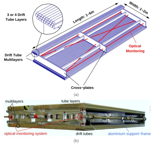
3.3 Monitored Drift Tube Chambers . . . 28
3.3.1 Drift Tube Principle . . . 29
3.3.2 Chamber Design . . . 30
3.3.3 MDT Chamber Electronics . . . 32
3.3.4 MDT Chamber Naming Scheme . . . 34
3.4 Trigger and Data Acquisition . . . 34
4 Calibration of the MDT Chambers 37 4.1 Introduction . . . 37
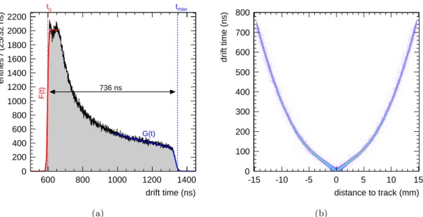
4.2 The Drift Time Spectrum . . . 39
4.3 The MDT Calibration Model . . . 41
4.3.1 Required Statistics . . . 44
4.3.2 Muon Calibration Stream . . . 44
4.3.3 Performance Goals . . . 44
4.4 Calibration of the Space-to-Drift-Time Relationship . . . 45
v
vi Contents
4.4.1 Integration Method . . . 45
4.4.2 Principle of Autocalibration . . . 46
4.5 Autocalibration with Curved Tracks . . . 47
4.5.1 Working Principle . . . 48
4.5.2 Curved Track Fit . . . 49
4.5.3 Sensitivity of the Residuals to the Drift Radii . . . 51
4.5.4 The Correction Function . . . 51
4.5.5 Iteration and Convergence . . . 52
4.5.6 Fixed Points . . . 52
4.6 Simulated Performance of the Autocalibration . . . 53
4.6.1 The Dataset for the Performance Tests . . . 54
4.6.2 Testing Procedure . . . 55
4.6.3 Determination of the Convergence Criterion . . . 58
4.6.4 Dependence on the Start Values . . . 60
4.6.5 Tuning the Autocalibration . . . 64
4.6.6 Standard Autocalibration Procedure . . . 66
4.6.7 Dependence on Statistic . . . 67
4.6.8 Calibration of the Full Spectrometer . . . 69
4.7 Systematic Effects . . . 69
4.7.1 Effect of the Drift Time Resolution . . . 69
4.7.2 Effect of the Accuracy of the t 0 Determination . . . 71
4.7.3 Effect of t 0 -Shifts within an MDT Chamber . . . 72
4.7.4 Effect of the Chamber Geometry . . . 75
4.8 Influence on Momentum Resolution . . . 76
4.8.1 Average Momentum Resolution of the Muon Spectrometer . . . 77
4.8.2 η- and φ-Dependence of the Momentum Resolution . . . 81
4.9 Test of the Autocalibration with Cosmic Ray Muons . . . 84
4.9.1 Cosmic Muons in ATLAS . . . 85
4.9.2 Datasets from Combined Cosmic Runs . . . 87
4.9.3 Autocalibration with Cosmic Muons . . . 88
4.9.4 Autocalibration with Magnetic Field . . . 92
4.10 Summary . . . 95
5 Search for LFV Decays τ τ τ → → → µµµ µµµ µµµ with ATLAS 97 5.1 Introduction . . . 97
5.2 Simulation of the Decay τ → µµµ . . . 98
5.3 Production of τ Leptons at the LHC . . . 99
5.3.1 Production of τ Leptons in Heavy Meson Decays . . . 99
5.3.2 Gauge Boson Decays . . . 100
5.4 Signal Event Topology and Detector Acceptance . . . 100
5.4.1 Kinematic Properties of the Signal Events . . . 101
5.5 Background Processes . . . 103
5.5.1 Background from Charm Decays . . . 105
5.5.2 Background from Beauty Decays . . . 106
5.6 Simulation of the Detector Response . . . 108
5.7 Trigger Performance . . . 108
5.7.1 Efficiency for τ → µµµ of the First-Level Muon Trigger . . . 108
Contents vii
5.7.2 Efficiency of the High-Level Triggers . . . 109
5.8 Reconstruction of Physics Objects and Detector Performance . . . 111
5.8.1 Muon Reconstruction . . . 111
5.8.2 Reconstruction of the Secondary Vertex . . . 116
5.8.3 Missing Energy Reconstruction . . . 116
5.8.4 Event Display of a τ → µµµ Decay . . . 117
5.9 Signal Selection Criteria . . . 117
5.9.1 Event Pre-Selection . . . 118
5.9.2 Signal Selection . . . 118
5.10 Estimation of the b ¯ b Background Rate. . . 126
5.11 Error Estimation . . . 129
5.11.1 Expected Statistical Uncertainties . . . 129
5.11.2 Theoretical Uncertainties . . . 129
5.11.3 Expected Systematic Uncertainties . . . 129
5.12 Upper Limit Estimation . . . 133
5.12.1 Statistical Method . . . 133
5.12.2 Results . . . 135
6 Summary 137 A Momentum Measurement with the ATLAS Muon Spectrometer 139 B MDT Chamber Naming Scheme 143 C Autocalibration with Curved Tracks 145 C.1 Analytic Expression for the Residual . . . 145
C.2 Sensitivity to the Measured Drift Radii . . . 147
D The Lorentz Angle Correction Function 149
Bibliography 161
Chapter 1
Introduction
Exciting years are awaiting the research field of particle physics. The Large Hadron Collider (LHC), the most powerful particle accelerator ever constructed, has started its operation at the European Laboratory for Particle Physics (CERN 1 ). It is designed to accelerate proton beams up to 7 TeV, allowing for proton-proton collisions with a centre- of-mass energy of 14 TeV. With these collisions, particle physicists from all around the world hope to find the answers to the most fundamental questions about the laws of na- ture such as the experimental prove of the last undetected particle of the Standard Model of particle physics: the Higgs boson. This discovery is crucial for the validation of the cur- rent understanding of matter, as this particle is supposed to give mass to all fundamental particles. Equally interesting questions concern phenomena beyond the Standard Model.
The hope is to find hints towards an even more fundamental theory of nature, including for example Supersymmetry which can provide a promising dark matter candidate and elegantly solves the hierarchy problem.
Colliding highly energetic protons is only one part of the exercise, the other one is the meticulous reconstruction of the processes occurring in the collisions. For this purpose, the LHC is equipped with four particle detectors. The largest one is ATLAS 2 , a general pur- pose detector which has been designed to exploit the full range of physics accessible at the LHC. Among its most distinct features is the muon spectrometer in a toroidal magnetic field created by superconducting air-core magnets. Since muons are produced in many interesting physics processes at the LHC, the precision of the momentum measurement of the muon spectrometer plays an important role.
After an introduction of the main properties of the LHC and ATLAS (Chapter 3) a pre- cise method for the calibration of muon drift chambers in magnetic fields is presented in Chapter 4. Especially for muon momenta above about 100 GeV/c, the muon chamber calibration is one of the dominating contributions to the muon spectrometer resolution.
The second part of this work is dedicated to the search for lepton flavour violating decays τ → µµµ. Lepton flavour violation is predicted by almost every extension of the Standard Model, including supersymmetric and so-called Little Higgs models. The lepton flavour violating decay rates predicted by these theories are becoming accessible at new colliders like the LHC. Chapter 2 gives an overview about lepton flavour violation in the Standard Model and in selected theories beyond the Standard Model. The LHC will produce about
1
CERN - Conseil Europeen pour la Recherche Nucleaire.
2
ATLAS - A Toroidal LHC ApparatuS.
1
2 Chapter 1. Introduction
10 12 τ leptons during one year of stable data-taking, which motivates the study of the
ATLAS sensitivity to the neutrinoless decay τ → µµµ presented in Chapter 5. After dis-
cussing the various sources of τ leptons in proton-proton collisions, a possible strategy for
this search and the expected upper limit on the branching ratio accessible by ATLAS are
discussed.
Chapter 2
Theoretical Background
2.1 The Standard Model of Particle Physics
The Standard Model forms the theoretical basis for the current understanding of the fun- damental particles and forces. According to the Standard Model, all matter consists of twelve fundamental fermions with spin 1 / 2 , six quarks and six leptons, which are grouped in three generations, each containing a quark and a lepton doublet. The first generation contains the up (u) and the down (d) quark and the electron (e) with the electron neutrino (ν e ), the second the charm (c) and the strange (s) quark, the muon (µ) and the muon neutrino (ν µ ) and the third the top (t) and the bottom (b) quark, the tau lepton (τ ) and the tau neutrino (ν τ ). Charged fermions of the second and third generation are heavier than the fermions of the first generation and unstable. The matter surrounding us on earth is entirely composed of first-generation particles.
Interactions between the fundamental particles are described by the exchange of twelve spin 1 bosons. The electromagnetic interaction is mediated by the massless photon (γ ), the weak interaction by the massive Z 0 and W ± bosons and the strong interaction by eight massless gluons (g 1 , ..., g 8 ). The Standard Model does not include the gravitational force as there is no satisfying quantum theory of gravitation yet. As the gravitational force is very weak compared to the other three forces, it can be neglected in the descrip- tion of elementary particle physics at current accelerator energies, at least for only three spacial dimension, but plays an important role in cosmology. The fundamental particles and interactions are summarized in Table 2.1.
Besides the twelve bosons mediating the forces, the theory also requires the existence of a scalar particle, the Higgs boson (H), to give rise to the masses of the Z 0 and W ± bosons and of the fermions in the so-called Higgs mechanism associated with the spontaneous breaking of the electroweak gauge symmetry. The Higgs boson is the only still undiscov- ered particle of the Standard Model.
Symmetry plays an important role in particle physics. All fundamental interactions of the Standard Model are described by gauge theories with the three symmetry groups
SU (3) C ⊗ SU (2) L ⊗ U (1) Y
for the strong interaction (Quantum Chromodymamics) and the unified weak and elec- tromagnetic interactions (Elektroweak Theory). According to Noether’s theorem [2], con-
3
4 Chapter 2. Theoretical Background
Table 2.1: The twelve matter particles (fermions) of the Standard Model and the four fundamental interactions with the corresponding mediators (gauge bosons). Gravitation is not included in the Standard Model and only listed for comparison. The undiscovered scalar Higgs boson H is not included in the table. Given masses coincide with the Particle Data Group [1].
Matter particles (spin 1 / 2 ) Force mediating particles (spin 1)
(Mass in GeV) (Mass in GeV)
Generation
Force Relative
Mediator
1 2 3 strength
L ep to n s ν e ν µ ν τ
Electromagnetic 10 − 2 γ
(∼0) (∼0) (∼0) (0)
e µ τ
Strong 1 g 1 , ..., g 8
(0.0005) (0.1) (1.8) (0)
Q u ar k s u c t
Weak 10 − 13 W ± , Z 0
(0.004) (1.5) (174) (81), (91)
d s b
Gravitation 10 − 38 Graviton (spin 2)
(0.007) (0.15) (4.7) (0)
tinuous symmetries of the action in a physical system lead to corresponding conservation laws and hence, to associated conserved quantum numbers in a quantum theory.
2.1.1 Quantum Chromodynamics
Among the fundamental fermions, only the quarks are participating in the strong inter- action which is described by the theory of Quantum Chromodynamics (QCD) [3–5]. In analogy to Quantum Electrodynamics (QED), the concept of colour charges was intro- duced to describe the strong interaction. In contrast to QED, which has only one electric charge and one massless neutral gauge boson, the photon, QCD requires three colour charges (commonly called red, green, blue) and eight massless gluons as force-mediating gauge bosons. The gluons carry combinations of colour and anti-colour charges and thus interact with each other themselves via the strong force.
The underlying gauge symmetry group of QCD is SU (3) C . The strong gauge coupling constant α s is the only free parameter of the theory. The non-abelian nature of SU (3) C and the resulting self-interaction of the gluons entail important implications of the the- ory: asymptotic freedom of quarks and gluons at short distances and their confinement in hadrons.
The strong coupling constant α s is a function of the energy scale or momentum transfer Q
of the process. With increasing energy scale, α s (Q 2 ) decreases and vanishes asymptotically
for Q → ∞ (asymptotic freedom). In contrast, at low energy scales or large distances be-
tween coloured particles, α s diverges. This behaviour is related to the phenomenon that no
free colour carrying particles exist and they are rather confined in hadrons. When colour
charges are separated from each other, the energy density eventually becomes large enough
that quark-antiquark pairs are created from the vacuum, leading to the so-called fragmen-
tation of quarks and gluons into hadrons, the hadronization. The observed hadrons are
colour neutral (white) and can be classified either as quark-antiquark (meson ) or three-
2.1. The Standard Model of Particle Physics 5
quark (baryon) bound-states.
2.1.2 The Electroweak Theory
The Standard Model is inspired by the local gauge invariant electromagnetic field theory of Quantum Electrodynamics (QED) which is based on the U (1) em symmetry group which leads to the conservation of the electric charge quantum number. In addition, the local gauge invariance also necessitates the introduction of an associated massless vector field, the photon.
The breakthrough in describing the weak interaction was achieved in the 1960’s by Glashow [6], Weinberg [7] and Salam [8] by unifying the weak with the electromagnetic interaction in the Electroweak or GWS Theory. This theory is based on the local gauge symmetry group SU (2) L ⊗ U (1) Y , which arranges the fundamental fermions in three gen- erations of left-handed doublets and right-handed singlets of the fundamental SU (2) L representation. It comprises one U (1) Y gauge field B µ and three SU (2) L or weak isospin gauge fields W µ i (i = 1, 2, 3). B µ couples to both left- and right-handed fermion fields, ψ L and ψ R , via the weak hypercharge Y , while the W µ i gauge fields only couple to the left-handed components. The left-handed projections of the fermion fields form the weak isospin doublets
ψ L = ν ℓ
ℓ −
L
, q u
q d
L
, (2.1)
with the weak eigenstates ℓ = e, µ, τ , ν ℓ = ν e , ν µ , ν τ , q u = u, c, t and q d = d, s, b. The quark mass eigenstates (q u ′ , q ′ d ) are related to the weak eigenstates (q u , q d ) via unitary transformations and interact weakly via the Cabbibo-Kobayashi-Maskawa (CKM) mixing matrix:
u ′ , c ′ , t ′
·
V ud V us V ub V cd V cs V cb V td V ts V tb
| {z }
CKM matrix
·
d ′ s ′ b ′
. (2.2)
The right-handed projections form SU (2) L singlets:
ψ R = ℓ R , ν ℓR , q uR , q dR . (2.3) The distinction between left- and right-handed fermion fields corresponds to the maximal parity violation by the weak interaction. The individual fermions are characterized by the quantum numbers J and J 3 of the weak isospin vector J = (J 1 , J 2 , J 3 ) and the weak hypercharge Y . The electric charge is given by the Gell-Mann-Nishijima relationship
Q = J 3 + Y
2 . (2.4)
An overview of the fermion multiplets of the electroweak interaction and their quantum numbers is given in Table 2.2.
The gauge invariant Lagrangian of the electroweak theory L ew can be written as sum of
the gauge field term L g and the fermion term L f and of two additional terms L h and L y
6 Chapter 2. Theoretical Background
Table 2.2: Fermion multiplets of the electroweak gauge symmetry with their quantum num- bers. Because weak isospin and hypercharge commutate, the third component J 3 of the weak isospin is assigned such that the weak hypercharge is the same within each doublet fulfilling the Gell-Mann-Nishijima relationship.
Fermion Multiplets J J 3 Y Q
L ep to n s
ν e e −
L
ν µ µ −
L
ν τ τ −
L
1 / 2 1 / 2 − 1 0
1 / 2 − 1 / 2 − 1 − 1
e − R µ − R τ R − 0 0 − 2 − 1
Q u ar k s
u d
L
c s
L
t b
L
1 / 2 1 / 2 1 / 3 2 / 3 1 / 2 − 1 / 2 1 / 3 − 1 / 3
u R c R t R 0 0 4 / 3 2 / 3
d R s R b R 0 0 − 2 / 3 − 1 / 3
which introduce masses for the weak gauge bosons according to the Higgs mechanism [9]
and for the fermions via the Yukawa interactions with the Higgs field, respectively:
L ew = L g + L f + L h + L y , (2.5)
which will be described in the following.
Gauge Field Term L g
The gauge field term of the electroweak Lagrangian reads L g = − 1
4 W µν i W i µν − 1
4 B µν B µν (2.6)
With the field-strengths defined by
W µν i = ∂ µ W ν i − ∂ ν W µ i + gǫ ijk W µ j W ν k , (2.7)
B i µν = ∂ µ B ν − ∂ ν B µ , (2.8)
where g is the weak SU(2) L gauge coupling constant, ǫ ijk the totally antisymmetric pseu- dotensor, W µ i (i = 1, 2, 3) the vector field triplet required by the local SU (2) L gauge symmetry and B µ the vector gauge field of the U (1) Y gauge theory corresponding to the weak hypercharge Y .
Linear combinations of the four gauge fields B µ and W µ i lead to the observable gauge bosons γ, Z 0 and W ± :
A µ Z µ
=
cos θ W sin θ W
− sin θ W cos θ W
B µ W µ 3
, (2.9)
W µ ± = 1
√ 2 W µ 1 ± iW µ 2
, (2.10)
with the weak mixing or Weinberg angle θ W determined by the SU (2) L and U (1) Y coupling constants g and g ′ according to
cos θ W = g
p g 2 + g ′ 2 . (2.11)
2.1. The Standard Model of Particle Physics 7
Fermion Term L f
Interactions between fermions and the gauge fields are described by the Lagrangian L f = i ψ ¯ L γ µ D µ ψ L + i ψ ¯ R γ µ D µ ψ R (2.12) where γ µ are the Dirac matrices and D µ the covariant derivatives which ensure the local gauge invariance of the theory:
D µ = ∂ µ + igJ i W µ i + ig ′ Y B µ . (2.13) For the left-handed fermion fields applies
D µ ψ R =
∂ µ + ig σ i
2 W µ i + ig ′ Y 2 B µ
ψ L , (2.14)
where σ i denote the Pauli-matrices, while for the right-handed fermions the covariant derivative is given by
D µ ψ R =
∂ µ + ig ′ Y 2 B µ
ψ R . (2.15)
Up to this point, all weakly interacting matter and force mediating particles are included in the theory. However, it has the severe problem that the theory contains no mass terms, which are forbidden by the electroweak gauge symmetry, in contradiction to the observations.
Higgs Term L h
A possible solution is the so-called Higgs mechanism which allows for massive gauge bosons without violating the local electroweak gauge symmetry of the Lagrangian L ew by intro- ducing a new complex scalar field
φ = φ +
φ 0
(2.16) with hypercharge Y = 1 which couples to the electroweak gauge bosons and has a non- vanishing vacuum expectation value. It is described by the Lagrangian
L h = (D µ φ) † (D µ φ) − V (φ) (2.17) where D µ is the covariant derivative introduced in Equation (2.13) and V (φ) the self- interaction potential of the scalar field
V (φ) = µ 2 φ † φ + λ(φ † φ) 2 , (2.18) where µ and λ are free parameters. For µ 2 < 0, the ground state φ 0 (vacuum) is infinitely degenerated under the electroweak gauge transformations with vacuum expectation value
| φ 0 | =: v / √ 2 different from zero with v =
r − µ 2
λ . (2.19)
8 Chapter 2. Theoretical Background
By selecting one ground state of the scalar field the electroweak gauge symmetry is spon- taneously broken. Three of the four components of the Higgs doublet become the lon- gitudinal polarization components of the electroweak vector bosons, which then become massive. Only one component of the Higgs doublet remains and manifests itself as a mas- sive neutral scalar, the Higgs boson H. The masses of the physical weak vector bosons are given by the gauge couplings g and g ′ and the vacuum expectation value of the Higgs field,
M W = 1
2 gv, M Z = 1 2
p g 2 + g ′ 2 v. (2.20)
Thus, the ratio of the masses of the Z 0 and W ± bosons is related to the electroweak coupling constants alone, independent of the Higgs potential:
M W
M Z = g
p g 2 + g ′ 2 = cos θ W . (2.21) The mass of the Higgs boson is given by
m H = p
− 2µ 2 . (2.22)
Yukawa Term L y
Fermion masses are generated by Yukawa couplings of the fermion spinor fields to the scalar field φ. For instance, for the first generation of leptons the corresponding Yukawa term is:
L y = − g e
(¯ ν e , e) ¯ L φe R + ¯ e R φ † ν e
e
L
(2.23) which becomes after spontaneous symmetry breaking in the unitary gauge
L y = − m e ee ¯ − g e
√ 2 ¯ eeH (2.24)
with g e denoting the Yukawa coupling constant of electrons and m e = g
ev / √ 2 . In general, the masses of the fermions f are given by
m f = g f v
√ 2 . (2.25)
2.1.3 Physics Beyond the Standard Model
The Standard Model of particle physics is very successful in describing experimental data at the highest precision. However, an extension of the model seems to be unavoidable due to several limitations, among which:
• The fourth known interaction, the gravitation, is not included in the theory.
• According to the current state of knowledge, only about 5 % of the mass in the
universe is described by the fermions of the Standard Model while 23 % consist of
so-called dark matter and 72 % of dark energy not included in the Standard Model.
2.2. Lepton Flavour Violation in the Standard Model 9
• Radiative corrections quadratically diverging with the energy scale drive the Higgs boson mass to the largest possible scale, eventually the Planck scale of 10 19 GeV.
However, the electroweak precision measurements indicate a Higgs boson mass near the electroweak scale ( ∼ 100 GeV) [10]. Thus the quadratic divergence has to be compensated with unnaturally high accuracy, referred as fine tuning, to keep m H at the electroweak scale.
So far no experimental evidence for physics beyond the Standard Model has been found, but further insight is expected from measurements by the LHC experiments.
2.2 Lepton Flavour Violation in the Standard Model
Besides the conserved charge quantum numbers of the gauge interactions—colour charge, weak isospin and weak hypercharge—additional conserved quantities and corresponding symmetries exist in the Standard Model. Lepton number conservation was proposed by Konopinski and Mahmoud [11] to explain why certain processes are allowed and others seem to be forbidden. The value L = +1 is assigned to every lepton and L = − 1 to the antileptons. All other particles are assigned to the lepton number L = 0. The lepton number is an additive quantum number, its sum is conserved in particle interactions in the Standard Model. An example is the beta decay with:
n → p + + e − + ¯ ν e
L : 0 = 0 + 1 − 1 (2.26)
The conservation of the lepton number alone is not sufficient to explain why for example the decay
µ → e − + γ
L : 1 = 1 + 0 (2.27)
has never been observed. Hence, it is required to conserve the lepton numbers L e , L µ and L τ for each generation separately, as for example in the decay of the muon:
µ → e − + ¯ ν e + ν µ L : 1 = 1 − 1 + 1 L e : 0 = 1 − 1 + 0 L µ : 1 = 0 + 0 + 1
(2.28)
Since the discovery of neutrino flavour oscillations it is known that the conservation of the lepton family number is not strict. A number of radio-chemical experiments includ- ing Homestake [12], GALLEX [13], GNO [14], and SAGE [15] and the real-time water Cherenkov experiments Kamiokande, Super-Kamiokande [16], and the Sudbury Neutrino Observatory [17] could prove a deficit in the flux of solar electron neutrinos while the total flux of neutrinos from the sun is consistent [17] with the expectations from the solar models.
This can only be explained by solar neutrino oscillations. Other experiments, in particular
the (Super-) Kamiokande experiment [18] discovered oscillations with atmospheric muon
neutrinos produced in cosmic ray induced air showers, the KamLAND [19] experiment with
muon neutrinos produced in nuclear reactors, and experiments like K2K [20], MINOS [21]
10 Chapter 2. Theoretical Background
τ µ
µ ¯ µ
W ν
jZ
(a)
τ µ
µ ¯ µ
ν
jW γ, Z
(b)
Figure 2.1: Feynman diagrams contributing to the lepton flavour violating decay τ → µµµ in the Standard Model with massive neutrinos which are able to change flavour periodically allowing changing neutral currents at a very low rate.
and OPERA [22] study neutrino oscillations in muon beams created by accelerators.
The discovery of the oscillating behaviour of the neutrino flavours has enormous conse- quences for the description of leptons in the Standard Model. It violates lepton fam- ily number or lepton flavour conservation, the neutrinos acquire masses and neutrino flavours mix in analogy to the CKM mixing of the quarks. The neutrino mass eigenstates ν j (j = 1, 2, 3) differ from the flavour eigenstates ν ℓ (ℓ = e, µ, τ ). Both are related by the unitary Pontecorvo-Maki-Nakagawa-Sakata (PMNS) mixing matrix:
ν e ν µ ν τ
=
U e1 U e2 U e3 U µ1 U µ2 U µ3 U τ1 U τ2 U τ3
| {z }
:= PMNS matrix
·
ν 1 ν 2 ν 3
(2.29)
The mixing of the neutrinos also gives rise to flavour violation for the charged leptons.
However, due to the unitarity of the mixing matrix, the tree level lepton decay is suppressed by the lepton sector analogue to the Glashow-Iliopoulos-Maiani (GIM) mechanism [23]
and only allowed via higher order loop processes. Figure 2.1 shows two examples of Standard Model loop processes contributing to the lepton flavour violating decay τ → µµµ.
According to [24], the processes in Figure 2.1(a) dominate with a decay rate ∝ log( m
2νj/ m
2W) while other contributions (see for example Figure 2.1(b)) are suppressed ∝ m
2νj/ m
2W. This leads to a branching fraction of:
B (τ → µµµ) ≥ 10 − 14 ,
depending on the neutrino mixing angles and mass differences. The τ → µµµ decay rate in the Standard Model is very small and beyond the sensitivity of current experiments.
The observation of such a lepton flavour violating τ decay would thus be an unambiguous sign of new physics beyond the Standard Model.
2.3 Lepton Flavour Violation in Theories Beyond the Standard Model
There is a large number of theories beyond the Standard Model in which the rate of lep- ton flavour violating decays is significantly increased due to new particles and interactions.
Mass-dependent couplings favour lepton flavour violation in the third generation. In gen-
eral, the radiative decay τ → ℓγ is more likely than the neutrinoless τ decay into three
2.3. Lepton Flavour Violation in Theories Beyond the Standard Model 11
τ µ
µ ¯ µ
˜ χ
0i˜ H, A ℓ
(a)
τ µ
µ ¯ µ
W
HZ
Hν
H(b)
Figure 2.2: Two examples of Feynman diagrams of the lepton flavour violating decay τ → µµµ in (a) the Minimal Supersymmetric extension of the Standard Model and (b) in the Littlest Higgs Model.
leptons mediated by γ since the additional γℓℓ-vertex leads to a suppression of the decay rate proportional to the fine-structure constant α. However, if the decay is mediated by a new heavy particle, then also τ → ℓℓℓ can be favoured. The extensions of the Stan- dard Model can be separated in two main classes: theories where charged-lepton flavour changing decays are still forbidden at tree level and theories where the tree level decays are allowed.
2.3.1 Models with Tree Level Suppressed Charged-Lepton Flavour Vi- olation
The first category encompasses extensions of the Standard Model in which charged-lepton flavour violation is still suppressed at the tree level. But new particles can enter at the loop level replacing, for example, ν j and γ, Z in Figure 2.1 and increasing the decay rate and branching ratio. Two examples of this class are the Minimal Supersymmetric extension of the Standard Model (MSSM) with massive neutrinos and the Littlest Higgs Model with T -parity conservation.
Supersymmetry (SUSY)
Supersymmetry is a symmetry between fermions and bosons added to the Standard Model.
This symmetry implies the existence of so-called superpartners for each particle of the Standard Model. Since the superpartners have not been observed so far, supersymmetry has to be broken in order to allow for superparticles much heavier than their corresponding Standard Model partners. A detailed introduction to Supersymmetry can be found, for example, in [25]. In the MSSM, two Higgs doublets have to be introduced to give masses to up- and down-type fermions which lead, after the spontaneous electroweak symmetry breaking, to five physical Higgs bosons, two charged (H ± ) and three neutral ones (h, H, A).
The superpartners of the Z boson (zino), the photon (photino) and the two neutral Higgs bosons (higgsinos) mix, resulting in four neutralinos ( ˜ χ 0 1 , χ ˜ 0 2 , χ ˜ 0 3 , χ ˜ 0 4 ) as mass eigenstates.
The superpartners of the charged leptons ℓ are the sleptons ˜ ℓ and the superpartners of
the quarks q are denoted squarks ˜ q. Dependent on the model parameters, charged-lepton
flavour violation can be mediated by the neutral Higgs bosons, neutralinos and sleptons
shown as example in Figure 2.2(a). Also the superpartners of the neutrinos (sneutrinos)
and charginos ( ˜ χ ± 1 , χ ˜ ± 2 ), mixing of superpartners of W ± (winos) and the two charged Higgs
bosons (charged higgsinos), can contribute to the loop processes.
12 Chapter 2. Theoretical Background
τ
˜ ν
µ µ ¯ µ
(a)
τ
H
−−µ ¯ µ µ
(b)
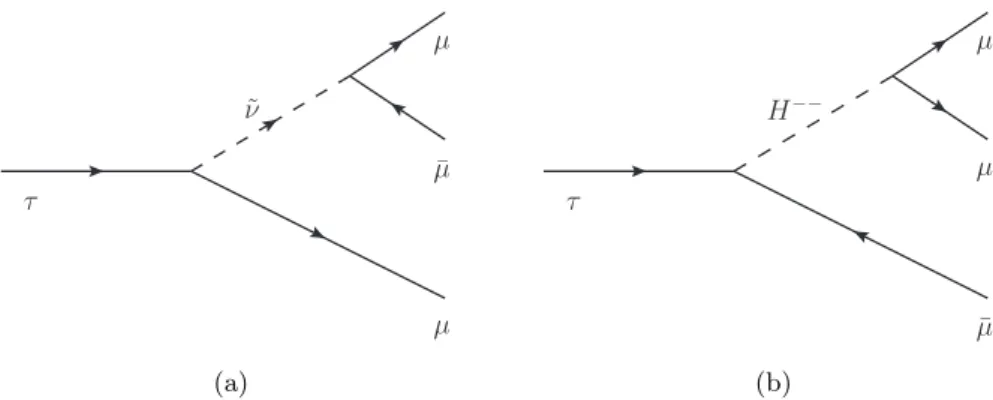
Figure 2.3: Two examples of tree level τ → 3µ decays in (a) supersymmetric models with R -parity violation and (b) models with doubly charged Higgs bosons.
A prediction of the branching ratio of the τ → µµµ decay for specific assumptions on the model parameters is [26, 27]:
B (τ → µµµ) . 10 − 9 . Littlest Higgs Model
The Littlest Higgs model is an alternative approach to generate electroweak symmetry breaking [28]. The theory predicts new mirror particles, for example ν ↔ ν H , Z ↔ Z H and W ↔ W H , at the TeV scale. To avoid problems with electroweak precision measurements, a discrete T -parity is introduced which allows only for pair production of the new particles (similar to the R -parity of supersymmetric models, see below). An example of a Feynman diagram contributing to the τ → µµµ decay is shown in Figure 2.2(b). Also for this model, the prediction of the branching ratio depends strongly on the model parameters and can reach up to [29, 30]:
B (τ → µµµ) . 10 − 8 .
2.3.2 Models with Tree Level Charged-Lepton Flavour Violation
In the second category of extensions of the Standard Model, also tree level lepton flavour violating decays are allowed leading to larger branching ratios for instance for the τ lepton decays into three muons via the exchange of new heavy particles.
Supersymmetry with R -Parity Violation
Conservation of the R -parity has been introduced in supersymmetric theories to suppress
lepton and baryon number violation which lead to the decay of the proton. In addition
it guarantees that the lightest supersymmetric particle is stable and thus provides an
excellent candidate for dark matter. Supersymmetric models with R -parity violation are
still possible within present experimental bounds on the proton lifetime and allow, for
instance, for couplings between the sneutrino (˜ ν) and the charged Standard Model leptons
(see Figure 2.3(a)) generating lepton flavour violation in the charged-lepton sector [31].
2.3. Lepton Flavour Violation in Theories Beyond the Standard Model 13
Models with Doubly Charged Higgs Bosons
Double charged Higgs Bosons (H ±± ) can give rise to lepton flavour violation including the decay τ → µµµ through processes as shown in Figure 2.3(b). The resulting branching ratios are on the order of [32]:
B (τ → 3µ) . 10 − 7 .
This work concentrates on the lepton flavour violating decay τ → µµµ as muons provide
a cleaner signature in the detector than electrons and the radiative decays τ → ℓγ. The
latter is expected to be very difficult to distinguish from the huge background of hadron
decays and bremsstrahlung photons.
Chapter 3
The Large Hadron Collider and the ATLAS Experiment
The Large Hadron Collider (LHC) [33] and the ATLAS experiment [34] were approved by the CERN council in December 1994. 15 years later, the first proton beams have been brought to collision on 23rd November 2009. The new particle accelerator will extend the accessible energy range with proton-proton collisions up to a centre-of-mass energy of
√ s = 14 TeV while reaching very high luminosities. ATLAS is one of the two general- purpose detectors at the LHC. CMS is the other one while ALICE and LHCb are dedicated to studies of heavy ion collisions and B meson physics, respectively. In this thesis simula- tions of the ATLAS detector performance are used to test a newly developed calibration algorithm for the precision muon drift chambers and to study the sensitivity on the decay τ → µµµ. In the following, the LHC and ATLAS are introduced.
3.1 The Large Hadron Collider
The Large Hadron Collider at CERN near Geneva, Switzerland, is the highest-energy proton-proton and heavy ion collider equipped with superconducting dipole magnets. It is installed in an underground tunnel of 26.7 km circumference, at depths between 45 and 170 m (see Figure 3.1). The processes of main interest for the LHC experiments are rare compared to the backgrounds of Standard Model reactions. For instance, the expected cross section for the production of a light Higgs boson is only on the order 10 pb—thus only 1 out of 10 11 proton-proton collisions contains a Higgs boson. Hence the challenge for the LHC is to provide an as high as possible event rate for the experiments. This rate is given by:
dN
dt = L · σ( √ s)
where σ is the cross section of the process studied depending on the centre-of-mass en- ergy √ s and L is the instantaneous luminosity which depends on the beam parameters according to
L = N b 2 n b f
A ,
15
16 Chapter 3. The LHC and ATLAS
LHC
SPS
PS 27 km
LHCb
ATLAS CMS
ALICE
Figure 3.1: Aerial view of the region around CERN. The locations of the LHC ring and the previous accelerators SPS and PS used for injecting protons into the LHC are indicated, as well as the locations of the four experiments ALICE, CMS, LHCb and ATLAS.
where f is the revolution frequency, n b the number of proton bunches per beam in the storage ring, N b the number of particles in each bunch and A the cross section of the beams.
The most important beam parameters for the peak luminosity of L = 10 34 cm − 2 s − 1 for which the LHC is designed are listed in Table 3.1.
In the first years, the LHC will run at lower energies and lower instantaneous luminosities to fully understand the accelerator and the experiments. After the incident during the commissioning phase in September 2008 the LHC program officially restarted on the 20th November 2009. After first collisions at √ s = 900 GeV in 2009, a two year period of operation at a centre-of-mass energy of √
s = 7 TeV takes place in 2010 and 2011 to be followed by a one year long shut-down to install additional safety and quench protection systems and to train the superconducting magnets for highest currents. This is necessary to ensure safe operation of the LHC up to the design beam energy.
The high interaction rates leads to a challenging environment for the experiments with very high radiation doses and particle multiplicities. Two of the four LHC experiments
• ATLAS (A Toroidal LHC ApparatuS) [34] and
• CMS (Compact Muon Solenoid) [35]
are general-purpose detectors designed to fully exploit the LHC physics potential up to
highest luminosity of L = 10 34 cm − 2 s − 1 . The other two have specialized physics programs
at lower instantaneous luminosities:
3.2. The ATLAS Experiment 17
• ALICE (A Large Ion Collider Experiment) is designed to study the creation of quark gluon plasma in highly energetic heavy ion collisions at a luminosity of L = 10 27 cm − 2 s − 1 [36].
• LHCb (Large Hadron Collider beauty) is devoted to the study of beauty physics at a luminosity of L = 10 32 cm − 2 s − 1 [37].
Table 3.1: LHC beam parameters for the peak luminosity of L = 10 34 cm − 2 s − 1 [33].
Unit Injection Collision Number of particles / bunch – 1.15 · 10 11
Number of bunches / beam – 2808
Circulating beam current (A) 0.582
Proton Energy (GeV) 450 7000
RMS transverse beam size (µm) 375.2 16.7
Stored beam energy (MJ) 23.3 362
Bunch crossing frequency (MHz) − 40
3.2 The ATLAS Experiment
This section gives an overview of the different detector technologies used in the ATLAS experiment and of their expected performance and introduces the most important physics goals.
3.2.1 Physics Goals and Detector Performance
The LHC provides a rich physics program, ranging from the measurement of Standard Model processes with high precision to a large variety of new physics searches. The most important studies are summarized below which serve to define the requirements for the ATLAS detector system.
Tests of the Standard Model The high luminosity and increased cross sections at the LHC compared to previous colliders 1 , enable precision measurements of QCD and electroweak processes, and of flavour physics. The top-quark will be produced at a rate of about 10 Hz at the peak luminosity providing the opportunity to test its couplings and spin.
Search for the Standard Model Higgs Boson This search is the main motivation for the LHC experiments and is a benchmark for the performance requirements of the ATLAS detector systems. Depending on the production and decay mode, the detection of the Higgs boson requires efficient identification and accurate energy and momentum measurement of electrons and muons. In addition, a hermetic detector for precise missing energy determination and the identification of b- and τ -jets is needed.
1
For instance, the Tevatron at the Fermilab close to Chicago, the highest energy hadron collider before
the LHC, achieves a peak luminosity of 3 × 10
32cm
−2s
−1with proton-anti-proton collisions at √ s =
1.96 TeV.
18 Chapter 3. The LHC and ATLAS
Discovery of Supersymmetric Particles In most models studied, the supersymmet- ric particles produced decay in cascades to Standard Model particles and the stable lightest supersymmetric particle (LSP). The typical signature therefore is large missing transverse energy due to the weakly interacting LSP together with several jets and, frequently, lep- tons.
Other New Physics Searches The LHC opens up a new energy range where searches for any kind of new particles and physics processes can be performed. Theories beyond the Standard Model predict for instance new heavy gauge bosons Z ′ and W ′ which are accessible up to masses of about 6 TeV. Searches for flavour changing neutral currents and lepton flavour violation through τ → µγ or τ → µµµ as well as measurements of rare B decays like B s 0 → µµ may open a window to new physics.
All processes mentioned above have small cross sections or decay rates which is the rea- son for the high design luminosity of the LHC. For the experiments this implies serious difficulties as the inelastic proton-proton cross section is about 80 mb. Hence the LHC will produce a total rate of up to 10 9 events per second with a bunch-crossing frequency of 40 MHz at the peak luminosity. This implies that every hard collision event will on average be accompanied by 23 inelastic interactions, an effect called pile-up. This leads to the following requirements to the detector:
• Fast, radiation-hard electronics and detector elements.
• High detector granularity is needed to cope with the high particle fluxes and to reduce the influence of pile-up events.
• Hermetic detector coverage around the interaction point up to the very forward re- gions in order to measure the decay products and the energy released in the collisions as completely as possible.
• High charged-particle energy and momentum resolution and reconstruction efficiency in particular for electrons and muons over a wide energy range from few GeV to about 1 TeV.
• High tracking accuracy close to the interaction region to assign particles to the primary hard scattering process, to select the decay products of unstable particles like B mesons or τ leptons and to identify pile-up events.
• Highly efficient trigger on electron, muon and jet signatures down to low momenta with sufficient suppression of the background.
3.2.2 The ATLAS Detector
This section provides an overview of the magnet system, the detector technologies and the trigger system of the experiment. The overall layout of the ATLAS detector is shown in Figure 3.2 with its main performance characteristics listed in Table 3.2. The detector is forward backward symmetric with respect to the interaction point. Like most of the general purpose particle detectors at colliders, it consists of three main measurement layers:
closest to the collision region is the inner tracking detector, followed by the calorimeters
and finally the muon spectrometer as outermost layer.
3.2. The ATLAS Experiment 19
Table 3.2: General performance characteristics of the ATLAS detector [34]. The units of E and p T are GeV and GeV/c. The pseudorapidity (η) covered by the sub-detectors are given for the particle measurement and, if applicable, in parentheses for the trigger.
Sub-detector Resolution | η |− range
Inner Tracker σ
pT/ p
T= 0.05 %/p T ⊕ 1 % < 2.5 EM calorimetry σ
E/ E = 10 %/ √
E ⊕ 0.7% < 3.2 (< 2.5) Hadronic calorimetry
barrel and end cap σ
E/ E = 50 %/ √
E ⊕ 3 % < 3.2 (< 3.2) forward σ
E/ E = 100 %/ √
E ⊕ 10 % 3.1 − 4.1 (3.1 − 4.1) Muon Spectrometer σ
pT/ p
T= 10 % at p T = 1 TeV < 2.7 (< 2.4)
The ATLAS Coordinate System
The right-handed ATLAS coordinate system is defined as follows:
• The origin at the nominal interaction point at the of the detector.
• The positive x-direction points towards the center of the LHC ring.
• The positive y-direction points upwards.
• The z-direction is oriented in direction of the beam line.
The azimuthal and polar angles are denoted by φ and θ. A commonly used variable in collider experiments is the Lorentz invariant pseudorapidity η:
η := − ln tan θ
2
. Distances in the η − φ space,
∆R := p
∆η 2 + ∆φ 2 ,
define opening angles between particles produced at the interaction point. Important variables are defined in the x-y plane transverse to the beam: The transverse momentum p T , the transverse energy E T and the missing transverse energy E T miss . These variables are Lorentz invariant under boosts along the z-direction which is important for hadron collider experiments as the collision products are usually boosted in beam direction. The transverse momenta and energies of all particles analysed in the detector should also add up to zero while energy is always lost in the longitudinal directions in the beam pipe.
3.2.3 The Magnet System
Special for the ATLAS detector is its superconducting magnet system consisting of a
solenoidal field for the inner detector and a toroidal magnetic field in the muon spectrom-
eter. The layout of the system is shown in Figure 3.3. The central solenoid [38] surrounds
the inner tracking detector and provides it with a homogeneous magnetic field of up to
2 T parallel to the beam line. To minimize the radiation lengths of material in front of
the calorimeters, the coil is only 10 cm thin and shares the vacuum vessel with the barrel
20 Chapter 3. The LHC and ATLAS
Figure 3.2: Cut-away view of the ATLAS detector. It measures 44 m in length, 25 m in diameter and weights almost 7 000 tons [34].
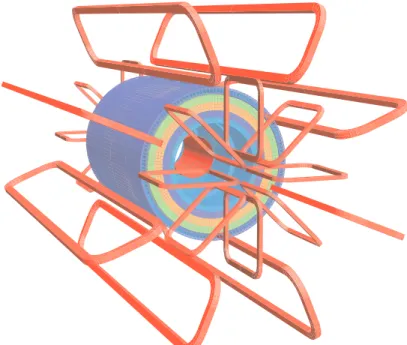
Figure 3.3: Schematic view of the superconducting coils of the ATLAS magnet system (red)
eight in the barrel part and eight in each end cap toroid. The iron in the calorimeter system
serves as return yoke for the central solenoid which lies inside the barrel calorimeter [34].
3.2. The ATLAS Experiment 21
electromagnetic calorimeter.
In ATLAS, the muon spectrometer has its own magnet system with a toroidal field config- uration with a mean field strength of 0.5 T. The system consists of three separate magnets:
• One barrel toroid consisting of eight 25 m long coils, each one in a separate cryostat.
• Two end cap toroids, each consisting of eight coils sharing a common cryostat.
Due to the limited number of coils, the toroidal magnetic is not uniform. It is essential for good momentum resolution to have knowledge about the field distribution with a relative accuracy on the order of (2 − 5) · 10 − 3 . The field configuration has two major advantages:
• The air-core magnet design minimizes multiple scattering of the muons inside the spectrometer.
• The momentum resolution is largely independent of the pseudorapidity up to the very forward regions.
Table 3.3 summarizes the main parameters of the ATLAS magnet system.
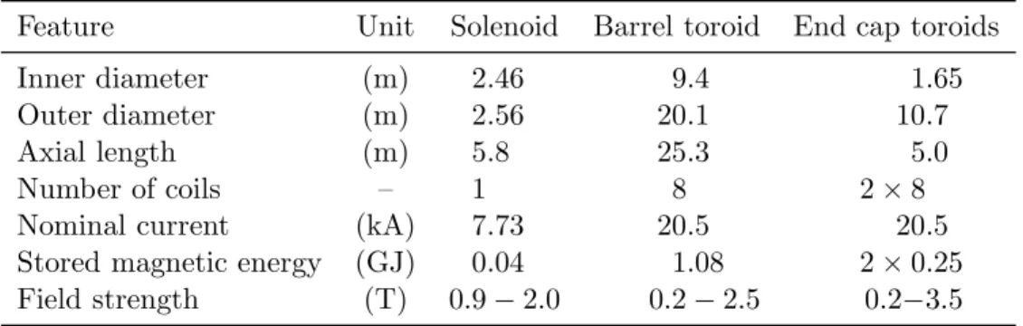
Table 3.3: Main Parameters of the ATLAS magnet system.
Feature Unit Solenoid Barrel toroid End cap toroids
Inner diameter (m) 2.46 9.4 1.65
Outer diameter (m) 2.56 20.1 10.7
Axial length (m) 5.8 25.3 5.0
Number of coils – 1 8 2 × 8
Nominal current (kA) 7.73 20.5 20.5
Stored magnetic energy (GJ) 0.04 1.08 2 × 0.25
Field strength (T) 0.9 − 2.0 0.2 − 2.5 0.2 − 3.5
3.2.4 The Inner Tracking Detector
The inner detector is designed to reconstruct trajectories of charged particles with high precisions and serves two main purposes: to measure the particle momenta and to deter- mine the origin of the particle (production vertex) and to distinguish between particles from the primary hard interaction, from a secondary vertex due to the decay of long lived particles or from additional inelastic proton-proton collisions. Since the inner detector is permeated by the field of the central solenoid, the tracks of charged particles are bent in the transverse plane allowing for momentum measurement from the track curvature.
The ATLAS inner detector combines three different but complementary detector technolo- gies providing efficient and accurate track reconstruction up to | η | = 2.5. Figure 3.4 shows a cut-away view of the inner detector.
Closest to the interaction region is the silicon pixel detector. To deal with the high
particle densities in the immediate vicinity of the proton-proton collisions, the pixel de-
tector has with 80.4 million read-out channels the highest granularity of all ATLAS sub-
detectors. It consists of three concentric cylinders around the beam axis in the central part
( | η | < 2.0) and of 3 disks perpendicular to the beam axis in each of the forward regions
22 Chapter 3. The LHC and ATLAS
Figure 3.4: Cut-away view of the ATLAS inner detector [34].
(2.0 < | η | < 2.5). Each pixel has the size of 50 × 400 µm allowing for a spatial resolution of the pixel sensors of 10 µm in the R − φ bending plane and of 115 µm in the z-direction in the barrel and radial direction in the end caps.
Table 3.4: Main parameters of the three detector technologies of the ATLAS inner detector.
Technology Point No. of space points No. of
resolution (µm) per track read-out channels
Pixel 10 (R − φ), 115 (z, R) 3 80.4 · 10 6
SCT 17 (R − φ), 580 (z, R) 4 − 9 6.3 · 10 6
TRT 130 (R − φ) 36 3 · 10 5
The pixel detector is surrounded by the semiconductor tracker (SCT) which consists of almost 16 000 silicon strip sensors with in total 6.3 million read-out channels. Four cylin- drical layers of small-angle stereo strip detectors in the barrel ( | η | < 1.1) and 9 disks in each of the end cap regions (1.1 < | η | < 2.5) measure at least 4 space points for each track.
The strip pitch of 80 µm allows for a spatial resolution of the strip sensors of 17 µm in the R − φ plane.
The outermost part of the inner detector is the Transition Radiation Tracker (TRT). This
gas detector consists of over 300 000 straw drift tubes. Polyimide tubes of 4 mm diameter
are filled with the gas mixture Xe/CO 2 /O 2 (70/27/3) at 5 − 10 mbar overpressure and
contain a 35 µm diameter gold-plated tungsten-rhenium anode wire in the center. The
straw tubes, with an intrinsic resolution of 130 µm, are arranged in 73 layers in the barrel
( | η | < 1.0) and in 160 layers in each end cap (1.0 < | η | < 2.0) contributing on average 36
3.2. The ATLAS Experiment 23
Figure 3.5: Cut-away view of the ATLAS calorimeter system [34].
space points to the track reconstruction. Between the tube layers polypropylene fibres and foils are embedded in the barrel and end caps, respectively, causing traversing electrons to emit transition radiation while the heavier muons and hadrons are passing essentially without radiation emission. By requiring the charge deposition around the track of a charged particle to exceed 2 GeV, electrons can be separated from hadrons, in particular from charged pions. The main parameters of the different detector technologies used in the inner detector are listed in Table 3.4.
3.2.5 The Calorimeters
All ATLAS calorimeters are sampling calorimeters with full φ-acceptance and η-coverage up to | η | = 4.9. They are characterized by high granularity and are realized with different active and absorber materials matched to their purpose. Figure 3.5 shows a cut-away view of the calorimeter system.
Located just outside the superconducting solenoid coil of the inner detector is the elec-
tromagnetic (EM-) calorimeter, consisting of a barrel part ( | η | < 1.5) and two end caps
(EMEC) extending up to | η | = 3.2, and complemented by two forward electromagnetic
calorimeters (FCal1) in the high pseudorapidity regions 3.2 < | η | < 4.9. The active
medium of all electromagnetic calorimeters is liquid argon which combines intrinsic ra-
diation hardness, stability over time and linear response. Special for the ATLAS EM-
calorimeters in barrel and end caps are the accordion-shaped lead absorbers and read-out
electrodes. This design allows for homogeneous response and fast signals without ineffi-
cient regions for read-out cables. For precise spatial and energy resolution, the electrode
segmentation in the η-region also covered by the inner detector ( | η | < 2.5) is very fine
24 Chapter 3. The LHC and ATLAS
(∆η × ∆φ = 0.025 × 0.025). The highest granularity of ∆η = 0.003 is implemented in the first of the three layers of the EM-calorimeter, the so-called η-strip layer.
The EM-calorimeters are surrounded by hadron calorimeters. In the barrel ( | η | < 1.1) and extended barrel (0.8 < | η | < 1.7) this is a scintillating tile calorimeter using steel absorbers and plastic scintillators as active medium. The tile calorimeter consists of three layers with a granularity of ∆η × ∆φ = 0.1 × 0.1. At higher pseudorapidities (1.5 < | η | < 3.2) two hadronic end cap calorimeters (HEC) are used for the energy measurement. They consist of copper plates with liquid argon as active medium and have the same granularity as the tile calorimeter for | η | < 2.5 and a granularity of ∆η × ∆φ = 0.2 × 0.2 for 2.5 < | η | < 3.2.
The largest pseudorapidities are covered by the forward hadron calorimeters (FCal2 and FCal3) with a tungsten absorber matrix with liquid argon filled boxes and with cell sizes of ∆x × ∆y = 3.3 × 4.2 cm 2 and ∆x × ∆y = 5.4 × 4.7 cm 2 , respectively.
The total thickness of the calorimeter system is more then 22 radiation lengths (X 0 ) and about 10 hadronic interaction lengths. This ensures a good energy resolution for highly energetic jets, precise reconstruction of the missing transverse energy and minimizes the punch through of particles to the muon spectrometer. The total number of read-out channels of the ATLAS calorimeter system is about 260 000. Its main parameters and quantities are summarized in Table 3.5.
Table 3.5: Parameters for the ATLAS calorimeters. The energy resolutions are from test- beam measurements [39–41] and well inside the specifications of ATLAS (see Table 3.2).
Name | η |− range Absorber / Energy resolution (E in GeV) active material (stochastic) (constant) EM <1.5 lead/LAr (10.1 ± 0.4) %/ √
E (0.2 ± 0.1) % EMEC 1.5 − 3.2 lead/LAr (10.1 ± 0.4) %/ √
E (0.2 ± 0.1) % Tile <1.7 steel/scint. (52.0 ± 1.0) %/ √
E (3.0 ± 0.1) % HEC 1.5 − 3.2 copper/LAr (70.6 ± 1.5) %/ √
E (5.8 ± 0.2) % FCal1 3.2 − 4.9 copper/LAr (28.5 ± 1.0) %/ √
E (3.5 ± 0.1) % FCal2+3 3.2 − 4.9 tung./LAr (94.2 ± 1.6) %/ √
E (7.5 ± 0.14) %
3.2.6 The Muon Spectrometer
Hadrons are interacting via the strong force and are thus absorbed almost completely in the calorimeters. Charged leptons on the other hand loose their energy mainly through ionization of atoms and bremsstrahlung in the Coulomb field of nuclei on their way through the detector. As the energy loss due to the latter is proportional to 1 / m
2, electrons are absorbed in the EM-calorimeters, while the 207 times heavier muons are traversing the inner parts of the detector mostly with only minor energy losses 2 and are detected in the muon spectrometer.
It is the muon spectrometer (see Figure 3.6) which defines the impressive size of the ATLAS detector with 44 m in length and 25 m in diameter. It is designed to provide an independent muon trigger and a high-precision muon momentum measurement up to
2
![Table 3.5: Parameters for the ATLAS calorimeters. The energy resolutions are from test- test-beam measurements [39–41] and well inside the specifications of ATLAS (see Table 3.2).](https://thumb-eu.123doks.com/thumbv2/1library_info/4015383.1541371/32.892.156.694.590.784/table-parameters-atlas-calorimeters-energy-resolutions-measurements-specifications.webp)
![Figure 3.8: Schematic layout of the muon trigger system. RPC2 and TGC3 are the reference (pivot) planes for the barrel and end cap triggers, respectively [34].](https://thumb-eu.123doks.com/thumbv2/1library_info/4015383.1541371/36.892.138.714.171.580/figure-schematic-layout-trigger-reference-planes-triggers-respectively.webp)
![Figure 3.12: Diagram of the MDT read-out electronics. Each CSM (Chamber Service Module) serves up to 18 mezzanine boards depending on chamber size, each MROD (Muon Read-Out Driver) up to 6 CSMs [51].](https://thumb-eu.123doks.com/thumbv2/1library_info/4015383.1541371/41.892.253.682.163.469/figure-diagram-electronics-chamber-service-module-mezzanine-depending.webp)
![Figure 4.5: Estimated single muon trigger rate and its contributions for a luminosity of L = 10 31 cm −2 s −1 depending on the muon p T threshold [52].](https://thumb-eu.123doks.com/thumbv2/1library_info/4015383.1541371/53.892.252.674.174.457/figure-estimated-single-trigger-contributions-luminosity-depending-threshold.webp)