TECHNISCHE UNIVERSIT ¨AT M ¨UNCHEN

Max-Planck-Institut f¨ur Physik (Werner-Heisenberg-Institut)

Study of the Performance of ATLAS Muon Drift-Tube Chambers in Magnetic

Fields and at High Irradiation Rates

Chrysostomos Valderanis

Vollst¨andiger Abdruck der von der Fakult¨at f¨ ur Physik der Technischen Universit¨at M¨ unchen zur Erlangung des akademischen Grades eines

Doktors der Naturwissenschaften (Dr. rer. nat.) genehmigten Dissertation.

Vorsitzender: Univ.-Prof. Dr. A. Ibarra Pr¨ ufer der Dissertation:

1. Priv.-Doz. Dr. H. Kroha

2. Univ.-Prof. Dr. L. Oberauer

1 Introduction 4

2 LHC and ATLAS 6

2.1 The accelerator complex . . . . 6

2.2 The ATLAS detector . . . . 7

2.2.1 Inner detector . . . 10

2.2.2 Calorimeter . . . 11

2.2.3 Muon spectrometer . . . 12

2.2.3.1 Rate environment . . . 14

2.2.3.2 Drift tubes . . . 15

2.2.3.3 MDT chambers . . . 16

2.2.3.4 Muon alignment system . . . 17

2.3 Performance reach of the muon spectrometer . . . 18

3 Test-beam Set-ups 20 4 MDT Properties without Background 23 4.1 Operation without magnetic field . . . 23

4.1.1 Measurement of the space-to-drift time relationship . . . 23

4.1.2 Measurement of the drift-tube spatial resolution . . . 25

4.1.3 Measurement of the drift-tube efficiency . . . 29

4.2 Drift-tube operation in magnetic fields . . . 30

4.2.1 Simple model for the B field dependence of r(t) . . . 31

4.2.2 Systematic uncertainties of the measurements . . . 36

4.2.3 Comparison of the measurements with model predictions . . . 36

5 MDT properties under Radiation Background 40 5.1 Rate dependence of the space drift-time relationship . . . 41

5.2 Rate depenence of the spatial resolution . . . 43

5.3 Rate dependence of the muon detection efficiency . . . 44

6 Conclusions 47

2

Introduction

This thesis is written in the context of experimental particle physics. The topic of experimental particle physics is the question of the fundamental constituents of matter and their interactions.

Ordinary matter is made of protons, neutrons, and electrons. While there are no hints for a substructur of electrons, protons and neutrons are not fundamental particle, but bound states of quarks. Electrons and protons are bound by the elec- tromagnetic interaction to atoms. Protons and neutrons as well as their constituent quarks take part in the strong interaction. At subatomic level also the the week interaction plays a role which is responsible for the β decay of nuclei.

The strong, electromagnetic, and weak interactions are part of the so-called

“Standard Model of the strong and electroweak interactions”. This model is able to described and predict the present results of particle physics experiments up to a precision of a few permill. In the Standard Model there are two groups of spin-

fermions, the leptons and quarks. The leptons take only part in the electromagnetic and weak interactions. There are six leptons in total, the electron, the muon and the τ lepton as electrically charged particles and their electrically neutral partners, the electron neutrino, the muon neutrino, and the τ neutrino which take only part in the weak interaction. There are also six quarks, the u, c, and t quarks and the d, s, and b quarks as their partners. The interactions between the fermions are mediated by spin-1 gauge bosons: massless gluons in case of the strong interaction, massless photons in case of the electromagnetic interaction, and massive Z and W bosons for the weak interaction. The Standard Model also predicts a scalar boson, the so-called “Higgs boson”. All massive particles obtain their masses through the interaction with the Higgs boson field.

The Higgs boson is the only particle in the Standard Model whose existance is still to be confirmed experimentally. The Large Hadron Collider (LHC) at the European Laboratory for Particle Physics CERN will make it possible to prove or disprove the existance of the Higgs boson. The LHC will also allow for probing predictions of theories beyond the Standard Model like its supersymmetric extensions.

The ATLAS detector will be used to study proton-proton collisions at large centre-of-mass energies of up to 14 TeV at the LHC. It is equipped with a muon

4

spectrometer for efficient muon identification and precise transverse momentum mea- surement with a resolution of 4% up to p

≈ 100 GeV/c and better than 10% up to p

≤ 1 TeV/c. The ATLAS muon spectrometer consists of a system of supercon- ducting air-core toroid coils generating a magnetic field delivering field integrals of about 2.5 Tm in the barrel part and up to 7 Tm in the end caps. The muon trajecto- ries in the muon spectrometer are measured with three layers of so-called monitored drift-tube (MDT) chambers whose shapes and relative positions are monitored by a system of optical sensors with micrometer accuracy. The MDT chambers are built of two quadruple layers of cylindrical drift tubes in the innermost layer and of two triple layers of drift tubes in the remaining two layers. The tubes have an outer diameter of 30 mm and a 400 µm thick tube walls made of aluminium. They are filled with a gas mixture of argon and carbon dioxide in the mixing ratio of 93:7 at an absolute pressure of 3 bar. The anode wire of 50 µm diameter is set to a voltage of 3080 V with respect to the tube walls leading to a gas gain of 20,000 and an average spatial single-tube resolution better than 100 µm. This corresponds to a spatial resolution of the chambers of better than 40 µm as required for 10%

momentum resolution at 1 TeV/c [1].

The magnetic field in the muon spectrometer is non-uniform, also within the muon chambers. The magnetic field B influences the electron drift inside the tubes:

the maximum drift time t

≈ 700 ns increases by approximately 70

B

. B varies by up to ± 0.4 T along the tubes of chambers mounted near the magnet coils which translates into a variation of t

with an amplitude of 45 ns [2]. The dependence of the space drift-time relationship must be taken into account in track reconstruction. Test-beam measurements presented in this thesis were needed to model this dependence with the required accuracy of 1 ns [3].

The operating conditions of the MDT chambers at the LHC design luminosity of 10

cm

s

are characterized by unprecedentedly high neutron and much higher γ background fluxes. The chambers are expected to show background counting rates of up to 500 s

cm

including all uncertainties in the prediction of the radiation background [4, 5]. The choice of the Ar:CO

gas mixture and the use of silicon free components in the gas system prevents the MDT chambers from aging [6, 7].

The high radiation background is known to degrade the spatial resolution of the tubes and the muon detection efficiency. The performance of the drift tubes at high γ irradiation background was studied with single tubes and preliminary read- out electronics for the first time in the late 1990s [8]. Measurements with a large ATLAS MDT chamber and the final read-out electronics finally be performed in the framework of this thesis in 2003 [9]. They are consistent with the earlier results using single tubes and have been followed up by measurements of the drift-tube behaviour in magnetic fields in 2004 [2].

This thesis contains the studies published in [2], [3], and [9] and extends them

by detailed comparisons of the measurements with predictions of the Garfield drift

chamber simulation programme [10].

LHC and ATLAS

The studies which will be discussed in the following chapters have been performed in the context of the ATLAS experiment [11] at the Large Hadron Collider (LHC)[12]

at the European Laboratory for Particle Physics CERN. The experiment is designed to study proton-proton collisions at 14 TeV centre of mass energy with the goal of understanding the mechanism of the electroweak symmetry breaking and of search- ing for physics processes not explained by the Standard Model of particle physics.

2.1 The accelerator complex

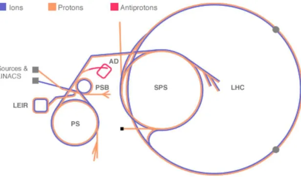
The protons colliding in the ATLAS detector are delivered to the collision point by an accelerator chain at CERN (see Figure 2.1) in a multi-step process [13]. The accelerator complex serves for the acceleration of different beam types (protons, antiprotons, ions, electrons).

In the proton-proton collisions at the LHC, the protons are first accelerated in the LINAC (LINear ACcelerator), which has a length of 80 m, and accelerates the protons to energies of 50 MeV. The protons are afterwards accumulated in the Proton Synchroton Booster (PSB), with a 160 m diameter, where their energy is increased to 1.4 GeV. The beam is then injected into the Proton Synchroton (PS), which has a diameter of 200 m, and accelerated to 25 GeV. It is at this point that the proton bunches take their final shape of 2.5 ns length with 25 ns latencies. Finally the beam is injected into the Super Proton Synchroton (SPS) and accelerated to 450 GeV before entering the LHC. The SPS ring has a diameter of 2.2 km.

The LHC accelerator is built as two parallel rings accelerating protons in opposite directions. The tunnel used for the LHC accelerator is a pre-existing previous gen- eration electron-proton collider (the Large Electron-Positron Collider (LEP)) with a circumferance of 27 km. In order to be able to steer the protons to energies of up to 7 TeV, a strong magnetic field of 8 T is required. This magnetic field cannot be achieved with conventional magnets, a new NbTi superconducting technology is used instead.

In addition to the so far highest beam energy, the LHC will also provide the

6

Figure 2.1: A schematic view of the CERN accelerator chain. The correct dimensions of different accelerators are given in the text.

highest luminosity L , which in the case of two colliding beams is defined as L = N

N

N

f

4πσ

σ

(2.1) where N

is the number of protons per bunch in the beam 1(2), N

is the number of bunches, f the revolution frequency and σ

is the transverse beam size of the bunch in the horizontal (vertical) plane. In the first two years of operation the LHC provided a luminosity of ∼ 10

cm

s

at 7 TeV centre-of-mass energy. In 2014 after a one year commisioning phase the collider will reach the design centre-of- mass energy of 14 TeV at the design luminosity of 10

cm

s

. The integrated luminosity

L = Z

L dt (2.2)

delivered by the accelarator until the end of 2012 will be ∼ 20 fb

. After changing to the high luminosity running one expects an annual integrated luminosity of 100 fb

.

2.2 The ATLAS detector

The ATLAS detector (A Toriodal LHC AparatuS) is one of the two multi-purpose

detectors located at the LHC tunnel. It is designed to explore the full range of

physics phenomena offered by the LHC.

T E R 2 . L HC AND A T L AS 8

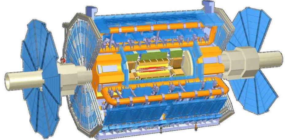
Figure 2.2: 3-dimensional view of the ATLAS detector.

In the first period of running at low luminosity the LHC is already going to be a high rate b- and t-quark factory. This will allow ATLAS experiment to perform detailed studies of the top quark properties together with investigations on the CP violation and B B ¯ mixing. The existence of the Higgs boson predicted by the electroweak symmetry breaking mechanism of the Standard Model can already be verified. Searches for the new physics can be started. However, many physics studies, like the study of the properties of the Higgs boson, require the high luminosity of 10

cm

s

in order to collect a sufficiently high number of signal events above background. Since the LHC is going to be primary a discovery machine, the ATLAS detector needs to provide as many signatures as possible so that robust and redudant physics measurements can be performed.

Finally, the ATLAS detector should have similar performance even at the highest possible luminosity that could ultimately be provided by the LHC accelerator, while searching for objects like new heavy gauge bosons W

and Z

, leptoquarks and the lighest stable supersummetric paricle (LSP).

The described physics goals lead to the following requirements on the detector design and performance:

• efficient tracking even at the highest luminosities for the lepton momentum and charge measurements, as well as the possibility for the b-quark tagging and τ-lepton and heavy-flavour vertexing and reconstruction;

• high-resolution, hermetic calorimeter for electron and photon identification and jet and missing energy measurements;

• precision muon spectrometer with a low-pt trigger capability at low luminosity as well as a stand-alone trigger at high luminosity.

The detector (shown in Figure 2.2) has a cylindrical shape following the beam pipe with a height of 26 m and a length of 43 m. One distinguishes the barrel region, where the components are arranged coaxially with respect to the beam axis and the end-cap region where the components are positioned perpendicular with respect to the beam axis. At this point it is proper to describe the coordinate system imposed on the detector. The origin of the coordinate system is at the interaction point in the centre of the detector. The z-axis coincides with the beam direction, while the x-axis points to the centre of the LHC ring and y-axis points upwards to the surface.

In this coordinate system the transverse momentum is defined as the projection of the momentum to the x-y plane. The azimuthial angle φ and the polar angle θ are defined with respect the the z-axis. In the following chapters we will often use a transformation of θ, the pseudorapidity η defined as

η = − ln tg θ

2 . (2.3)

For a particle with a mass much less than the transerve momentum, the pseudora-

pidity is a good aproximation for a relativistic equivalent of the particle’s velocity.

The ATLAS detector is divided into three subdetectors. The innermost subde- tector surrounding the beam pipe is the inner detector for the measurement of the charged particle tracks. The inner detector is surrounded by a hermetic calorimeter.

Finally, the outermost subdetector defining the size of the ATLAS detector is the muon spectrometer. In the following we will give a short introduction to each of those detectors.

2.2.1 Inner detector

The task of the inner detector is to reconstruct the tracks and vertices of charged particles in the event with high efficiency and resolution, contributing to the electron, photon and muon momentum reconstruction.

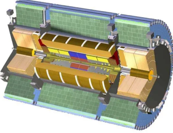
Figure 2.3: 3-dimensional view of the ATLAS inner detector.

The inner detector is contained in a solenoidal magnet with a central field of

2 T, providing a precise momentum measurement of the tracks. A three dimensional

cutaway view of the inner detector is shown in Figure 2.3. The outer radius of the

tracker cavity is 115 cm, fixed by the inner dimension of the cryostat containing

the liquid argon electromagnetic calorimeter, and the total length is 7 m, limited

by the position of the end-cap calorimetry. Mechanically the inner detector consists

of three units: a barrel part extending over 160 cm, and two identical end-caps

covering the rest of the cylindrical cavity. In the barrel, the detector layers are

arranged on concentric cylinders arround the beam axis in the region with | η | < 1,

while the end-cap detectors are mounted on disks perpendicular to the beam axis,

covering the pseudorapidity region up to | η | < 2.5. The precision tracking elements

are contained within a radius of 56 cm, followed by the continuous tracking, and finally the general support and service area at the outermost radius.

The momentum and vertex resolution targets require high-precision measure- ments to be made with fine-granularity detectors given the very large track density expected at the LHC. The highest granularity is needed around the beam pipe where for this reason the semiconductor pixel detectors are used. The resolution that can be achived by these detectors is 12 µm in transverse and 66 µm in longitudinal di- rection. However, the high cost of pixel detectors forbids their usage for more than a few layers. The pixel detectors are surrounded by a semiconductor tracker (SCT) in the form of the silicon microstrip detectors with resolution of 16 µm transverse to the beam and 580 µm in the longitudinal direction. The dense material of the semiconductor detectors contributes significanty to the particle scattering which re- duces the momentum resolution. In order to reduce the amount of material in the outermost part of the inner detector the gas detectors in the form of straw tube detectors with transition radiation measurenent (TRT) are used. The straw tubes diameter of 4 mm offers an almost continuous tracking. The position resolution offered by the TRT detectors is 170 µm in the transverse plane.

The combination of the semiconductor detectors with the straw tubes gives a very robust pattern recognition and a higher precision in both φ and z coordinates.

The straw hits at the outer radius contribute to the momentum measurement with a resolution similar to the semiconductor detector because the lower precision per point compared to the silicon detectors is being compensated by the large number of measurements and the higher average radius. The relative precision of the sep- arate measurements is well matched so that no single measurement dominates the momentum resolution. This means that the overall performance is robust, even in the event that a single system does not perform to its full specification.

2.2.2 Calorimeter

The task of the calorimeter is to trigger on and to provide accurate measurements of energy and direction of electrons, photons and jets and missing transverse mo- mentum of the event.

A three dimensional cutaway view of the calorimeter layout is shown in Fig- ure 2.4. This subdetector can be divided into electromagnetic and hadron calorime- ter. The barrel electromagnetic calorimeter is contained in the barrel cryostat, which surrounds the inner detector cavity. The solenoid which supplies the 2 T magnetic field in the inner cavity is integrated into the vacuum vessel of the barrel cryo- stat and is placed in front of the electromagnetic calorimeter. The electromagnetic calorimeter is contained in a cylinder of outer radius 2.25 m and a total length span- ning 6.6 m along the beam axis ( | η | < 1.475). The hadron calorimeter system has an outer radius of 4.23 m and a total length of 12.2 m, covering the pseudorapidity region of | η | < 1.475. Two end-cap cryostats house the end-cap electromagnetic and hadron calorimeters as well as the integrated forward calorimeter.

The requirements set on the ATLAS calorimeters combined with the intrinsically

Figure 2.4: 3-dimentional view of the ATLAS calorimeter.

difficult experimental environment in terms of particle fluxes expected over the pe- riod of operation (10 years), the distance between bunch crosses and collisions per bunch crossing has lead to the decision for liquid argon (LAr) sampling electromag- netic calorimeter with accordion shape absorbers and readout electronics. The LAr sampling technique is radiation resistant and provides long term stability of the de- tector with good energy resolution. The barrel hadron calorimeter is implemented as a sampling calorimeter which makes use of steel as the absorber material and scintillating plates read out by wavelength shifting fibres as the active medium. The highly periodic structure of the system allows the construction of a large detector by assembling smaller sub-modules together. At larger rapidities (in the end-cap region), where higher radiation resistance is needed, the intrinsically radiation-hard LAr technology is used for all the calorimeters. The hadron end-cap calorimeter is a copper-LAr detector with parallel plate geometry and the forward calorimeter is a dense LAr calorimeter with rod electrodes in a tungsten matrix.

2.2.3 Muon spectrometer

The muon spectrometer [14] is capable of stand-alone muon triggering and recon-

struction over a wide range of transverse momentum, pseudorapidity and azimuthal

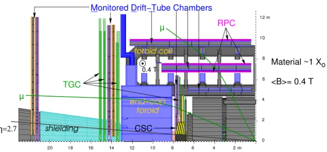
angle. The spectrometer layout is shown in Figure 2.5.

Figure 2.5: Schematic drawing of a quadrant of the ATLAS muon spectrometer.

The muon tracking is based on the magnetic deflection of muon tracks in a sys- tem of three large superconducting air-core toroid magnets. The spectrometer is instrumented with trigger and precision tracking chambers. In the pseudorapidity range | η | < 1.0 the magnetic bending is provided by a large barrel magnet con- structed of eight coils surrounding the hadron calorimeter. For 1.4 < | η | < 2.7 the muon tracks are bent by two smaller end-cap magnets inserted into both ends of the barrel toroid. In the intermediate interval 1.0 < | η | < 1.4 the magnetic field is pro- vided by a combination of the barrel and end-cap fields. This magnet configuration provides a field that is mostly orthogonal to the muon trajectories, while minimizing the degradation of the resolution due to multiple scattering. In the barrel region the sagitta of the tracks is measured by the precision chambers arranged in three cylindrical layers around the beam axis: at the inner and outer edges of the mag- netic volume and in the mid-plane. In the forward direction two disks of chambers are placed at the front and back faces of the end-cap magnets, with a third layer against the cavern wall to minimize the error in the calculation of the direction of the muon trace.

Over most of the pseudorapidity range, a precision measurement of the track

coordinates in the principal bending direction of the magnetic field is provided by the

Monitored Drift Tubes (MDT). At large pseudorapidities and close to the interaction

point, where higher rates and severe background conditions are expected, Cathode

Strip Chambers (CSC) with higher granularity are used. For the trigger system the

Resistive Plate Chambers (RPC) are used in the barrel and Thin Gap Chambers

(TGC) in the end-cap region. The RPC chambers are located on both sides of the

middle MDT station and on the outer side of the outer station. The TGC chambers

are located in three stations near the middle end-cap MDT station. Both types of

trigger chambers also provide a measurement of the track coordinate orthogonal to

the precision measurement (second coordinate).

Since a large part of this thesis is devoted to the performance of the MDT chambers, we are now going to discuss the relevant parts of the muon spectormeter in more detail.

2.2.3.1 Rate environment

The air-core design of the magnet system of the ATLAS muon spectrometer leads to high background hit rates in the muon detectors. The hits in the muon spectrometer have two sources, muons on the one hand and neutrons and photons on the other.

To the first class belong the muons coming from the primary collision products. This includes muons produced in the decays of heavy-flavour hadrons and gauge bosons (c, b, t → µX and W, Z, γ

→ µX). The first class of background hits includes also muons such as those coming from the decay in flight of light hadrons, where the muon is energetic enough to traverse the calorimeter or those muons that are coming from the hadronic debris produced in the calorimeter showers. A common feature of the muons belonging to this first category is the ime association to a given p-p collision.

Figure 2.6: Background fluxes of neutrons, photns, muons and pions in dependence

on the position in the muon spectrometer. The n and γ fluxes are in units of kHz/cm

and the µ and p fluxes are in units of Hz/cm

. [5]

The second most important class of background hits in the muon spectrometer are the low-energy neutrons, photons, electrons, muons and hadrons originating from the intraction of primary hadrons with the forward part of the detector and the forward elements of the LHC accelerator. These forward elements include the forward calorimeter, the shielding in the end-cap toroid, the beam-pipe and other machine elements. While most of the energy carried by these secondary particles is absorbed in the forward shielding, low energy neutrons wil escape the absorber and create via nuclear n-γ reactions, a low energy photon gas. Neutron and photon fluences have been computed taking into account the material distribution and the results are presented in Figure 2.6. Fluences tend to be isotropic in the barrel and thus create a ”particle gas”, while in the end-cap a substantial amount of the particles comes from the interaction point. The high background rates play a major role in the design of precision tracking chambers.

2.2.3.2 Drift tubes

The basic detection element used in the MDT chambers is a cylindrical aluminium tube of 30 mm diameter with a W-Re central wire of 50 µm diameter (Figure 2.7).

The tube length varies between 1 m and 6 m depending on its position in the muon spectrometer. The tube is filled with non-flamable gas composed of Ar(93%) and CO

(7%), at 3 bar absolute pressure. It is operated at 3080 V and the polarity is chosen such that the central wire is positive with respect to the outer cylinder.

Figure 2.7: Schematic view of a drift tube.

The operational principle of the drift tubes is the following. A muon crossing a drift tube ionizes the detector gas. A discrete number of primary ionizing collisions liberates electron-ion pairs in the gas. The electrons can have enough energy to further ionize the gas, producing secondary electron-ion pairs. The sum of the two contributions is called the total ionization. The number of primary ionizations, being a small number of independant events, follow a Poisson distribution.

If no external field were present, the charges produced by an ionizing event would quickly lose their energy in multiple collisions with the gas molecules and assume the average thermal energy distribution of the gas. In the case of the radial electric field E(r)

E = V

r ln

(2.4)

where a is the wire radius, b the inner tube radius and V the high voltage applied across the gas volume, a net movement of the clusters along the field direction is observed. The average velocity u of this slow motion is called the drift velocity and can be calculated as

u = e

2m Eτ (2.5)

where e(m) is the charge (mass) of the electon and τ is the mean time between the collisions, in general a function of the electric field E.

In the high-field region near the wire the drift electrons gain enough energy to ionize gas atoms such that the charge is multiplied in an avalanche process creat- ing new electron-ion pairs. The anode voltage is chosen such that the avalanche multiplication factor (gas gain) is 2 x 10

. The positive ion cloud moves from the avalanche zone towards the cathode and induces a current signal in the anode wire.

The electrons in the avalanche region are drifting to the wire and also induce a signal there. However, since their drift distance is of the order of the avanalche zone (100 µm), the electron signal is a sharp spike of about 100 ps length containing very little charge and can thus be neglected.

The current signal is read out on one side of the tube, amplified, shaped and discriminated. The output pulse of the discriminator is given to a time-to-digital converter (TDC) which measures the time difference between the muon pulse and a trigger signal (drift time). The drift time is converted to the radius of the closest approach of the track to the anode wire. The conversion is done by means of the space-time relation r(t). The r(t) relation is determined through the autocalibration procedure and will be discussed in more detail in Chapter 3. The drift radius in an individual tube only defines the circle to which the muon track was tangent. In order to reconstruct the muon tracks, the drift tubes are assembled into MDT chambers.

2.2.3.3 MDT chambers

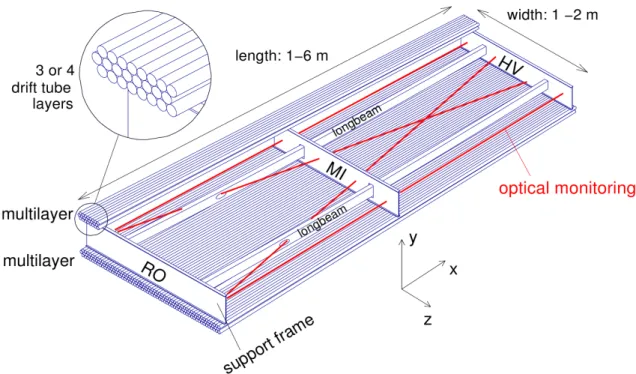
An MDT chamber (see Figure 2.8) consists of three or four layers (combined to a multilayer) of drift tubes on each side of a supporting space frame. There are between 30 and 72 tubes in each layer.

The supporting frame is a light-weight aluminium structure holding the drift tube layers. It consists of three cross plates, oriented perpendicular to the tube axis, and two longbeams, connecting the cross plates, oriented parallel to the tube axis. The two adjacent layers in one multilayer are shifted with respect to each other by half of the diameter of the tube, providing for unambiguous track reconstruction.

Since the accuracy of the muon reconstruction with MDT chambers depends on

the positioning accuracy of the tubes within the chamber, the chamber assembly

takes place on a flat robust granite table in a climatized room with temperature and

humidity control. The granite table provides a reliable reference for the position-

ing of mechanical assembly tools. The temperature and humudity control allows the

reproducibility of the mechanical chamber parameters during the chamber construc-

tion. Since after leaving the assembly table the chamber is going to be subject to

gravitational stresses that may deform it, an optical system is built into the chamber

Figure 2.8: Schematic view of a barrel MDT chamber.

during the construction phase so that the mechanical chamber deformations can be monitored. The light rays of the internal optical alignment system are shown in Figure 2.8.

2.2.3.4 Muon alignment system

The optimum performance of the muon spectrometer can only be reached if the positions of the chambers relative to each other along the muon track are known to a precision that is comparable to the intrinsic chamber resolution. The chamber alignment is therefore of prime importance. Given the large dimensions of the spectrometer, no attempt is made to actively re-position the chambers. Instead the relative positions of the chambers are monitored with optical systems and the position information is used to correct the measured track coordinates in the offline reconstruction software. The layout of optical alignment rays is shown in Figure 2.9.

The chambers in each of the three layers are combined in groups of two, forming a so called logical chamber unit. Four alignment rays connect the three logical chambers units of three different layers. The light rays traverse the chambers close to their four corners, to form a projective structure with respect to the interaction point.

Two more pairs of rays in the z-direction (”praxial lines”) offer more constraints in

finding the position of the chambers.

Figure 2.9: Layout of the light rays of the optical alignment system in the barrel sector of the muon spectrometer.

2.3 Performance reach of the muon spectrometer

The goal of the muon spectrometer is a muon momentum measurement with high resolution of 3-10% in a wide range of momenta from 10 GeV to 1 TeV. This sets the requirements on the perforamnce reach of the different building components of the muon spectrometer. The required mechanical accuracy of the wire positioning within the chamber is 20 µm (r.m.s.). The position resolution in an individual tube has to be better than 100 µm. Since each chamber is constructed with 6 or 8 layers, this translates into a track point resolution of < 40 µm in the chamber as a whole.

In addition the error introduced by the optical alignment system has to be smaller than the resolution of the chamber.

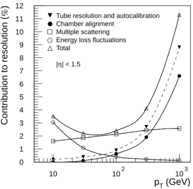
The expected momentum resolution of the muon spectrometer as a function of

the transverse momentum is shown is Figure 2.10, seperately showing the dominating

contributions to the resolution coming from the chamber resolution, alignment, mul-

tiple scattering and energy loss fluctuations. For high momenta (p

> 300 GeV/c),

the resolution is dominated by the precision with which the magnetic deflection is

measured, i.e. the resolution is determined by the intrinsic resolution. For moderate

momenta (30< p

<300 GeV/c), the resolution is increasingly limited by multiple

scattering. This contribution depends both on the amount of material traversed by

the muon and the distribution of that material along the track. For low momenta

(p

<30 GeV/c), the fluctuation of the energy loss become the dominant constraint

0 1 2 3 4 5 6 7 8 9 10 11 12

10 10² 10³

p

(GeV)

Contribution to resolution ( % )

Tube resolution and autocalibration Chamber alignment

Multiple scattering Energy loss fluctuations Total

|η| < 1.5

Figure 2.10: Momentum resolution of the muon spectrometer as a function of the transverse momentum p

. The different contributions to the resolution are specified.[14]

on the momentum measurement.

Test-beam Set-ups

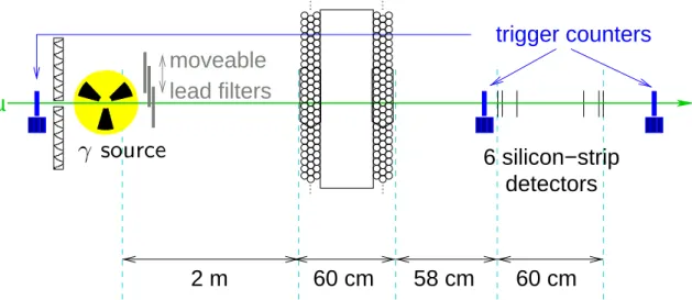
The measurements discussed in this thesis were carried out at the Gamma Irradi- ation Facility (GIF) at CERN [15] which provided a 90 GeV muon beam and a 664 GBq

Cs source emitting 66 keV γ rays used to simulate the ATLAS radiation background. The flux of γ rays to which the drift tubes were exposed during the measurements could be adjusted with movable lead filters in front of the opening of the source. Two experimental set-ups were installed in the GIF, one in 2003 and the other one in 2004 (see Figures 3.1 and 3.2, respectively). Common to both installations are the trigger system and the beam hodoscope.

60 cm 58 cm

60 cm

trigger counters

2 m

00 00 11 11 000 000

111 111 000 000

111 111 µ

6 silicon−strip detectors

00 00 00 11 11 11 00 00 00 11 11 11

moveable lead filters γ source

Figure 3.1: Schematic drawing of the experimental set-up in 2003. A full-size MDT chamber was operated in the GIF.

The beam hodoscope consists of two groups of three silicon strip detectors of 5 × 5 cm

active area separated by 60 cm. Each of the four inner strip detectors measures the horizontal positions of the incident muons with 10 µm accuracy. The two outermost detector planes measure the vertical muon positions with the same accuracy. In 2004, one of the vertical detectors had to be turned off due to very high leakage currents.

20

30 cm 1.5 m

000 000 111 111 00 00

11 11 000 000

111 111 µ

00 00 00 11 11 11 00 00 00 11 11 11

dipole magnet γ source

B ~

Figure 3.2: Schematic drawing of the experimental set-up in 2004. A small bundle of short drift tubes is mounted on a rotation table in the middle of the beam hodoscope inside a large dipole magnet. A bundle of 3.8 m long drift tubes is installed in front of the source outside the magnet for high-rate studies.

The beam hodoscope is enclosed by two fast scintillation counters with the same active area as the silicon detectors. A coincidence of these two counters with a 10 × 10 cm

scintillator counter mounted upstream in the beam and shielded against the radiation of the γ source provides the trigger and the start time for the drift- time measurements in the tubes. The jitter of the trigger time of less than 0.5 ns is negligible compared to the time resolution of the drift tubes of about 3 ns.

In 2003, one of the largest ATLAS MDT chambers was operated in the GIF with final read-out electronics. The chamber contains 432 drift tubes of 3.8 m length in two triple layers separated by 317 mm. It was installed at 2 m distance from the radioactive source. The sense wire of each drift tube is capacitively coupled to a chain of amplifier, shaper, and discriminator [16] on the MDT frontend electronics chips. A time-to-digital converter measures the arrival times of the signal with respect to the trigger time for each tube in a group of 24. Bipolar shaping with at peaking time of 15 ns is used. The discriminator threshold is adjustable and set to a value corresponding to 5 times the thermal noise originating from the 383 Ω termination resistor at the high-voltage connection end of the tubes. The signal pulse heights are measured by an analog-to-digital converter for each group of 24 channels.

Bipolar shaping was chosen in order to avoid baseline shifts of the analog signals caused by multiple hits in the presence of high radiation background in the ATLAS muon spectrometer. A consequence of bipolar shaping are multiple crossings of the discriminator threshold by the pulses. The secondary threshold crossings can be masked by an artificial dead time of 790 ns after the detected hit [2]. This is the baseline for the operation in ATLAS. The dead time is adjustable between 200 ns and 790 ns. The baseline value of 790 ns was used in the testbeam in 2003; testbeam measurements with the minimum dead time of 200 ns were performed in 2004.

In 2004, a bundle of 24 drift tubes of 3.8 m length was installed in the GIF

at 1.5 m distance from the γ source in order to study the drift tube performance

with the minimum dead time settng of the readout electronics. The other important

goal of the 2004 test-beam programme was the precise measurement of the influence

of the magnetic field on the space-to-drift time relationship of the tubes. For this

measurement, a chamber with 3 × 3 ATLAS drift tubes of 1.5 m length was installed

in the center of the beam hodoscope and operated in a magnetic dipole field of

uo to 0.9 T strength measured with a Hall probe mounted on the chamber. The

orientation of the magnetic field vector B ~ with respect to the direction of the anode

wires of the tubes could be varied by rotating the chamber inside the magnet.

Drift-Tube Properties in the

Absence of Radiation Background

In this Chapter, the space-to-drift time relationship, the spatial resolution, the pulse- height spectra, and the efficiency of the drift tubes of the ATLAS MDT chambers in the absence of background radiation will be discussed. First studies of the per- formence without magnetic field are presented, followed by the analysis of measure- ments inside a magnetic field. The drift tubes are operated, like in ATLAS, with a Ar:CO

(93:7) gas mixture at 3 bar absolute pressure and at a nominal temperature of 20

C.

4.1 Operation without magnetic field

Throughout the analysis muon trajectories are reconstructed with the data of the beam hodoscope independently of the muon chambers. The high spatial resolution of the silicon strip detector planes of the hodoscope allows for the determination of the positions of the muon tracks in the drift tubes with much better accuracy than the spatial resolution of the drift tubes.

4.1.1 Measurement of the space-to-drift time relationship

Figure 4.1 shows the drift time measured by a tube traversed by the muons as a function of the distance of the reconstructed hodoscope trajectory from the an- ode wire of the tube. Most of the data points populate a dark band whose contour reflects the space drift-time relationship. The space drift-time relationship is approx- imately linear for radii less than 5 mm corresponding to an average drift velocity of 0.05 mm ns

. The drift velocity drops continously with increasing radius above 5 mm and has a mean value of about 0.017 mm ns

in this region. The width of the dark band is a measure of the drift time resolution which is on the order of few nanoseconds. 7% of the data points lie below the dark band. These entries are caused by δ electrons which are knocked out of the tube walls by the incident muons leading to drift times shorter than the ones for the muon hits.

23

0 2 4 6 8 10 12 14 16 0

100 200 300 400 500 600 700

t (n s)

r

(mm)

Figure 4.1: Drift times measured by a tube traversed by muons as a function of the distance of the muons from the tube’s anode wire as reconstructed by the beam hodoscope. The MDT read-out electronics is operated with the maximum dead time of 790 ns.

The data analysis starts with a comparison of the measured space-to-drift time relationship to the prediction of the drift-chamber simulation programme ”Garfield” [10].

Garfield versions 8 and 9 are used. The most important difference between the two versions are the cross sections for the collisions of the drifting electrons with carbon dioxide molecules in the chamber gas. In the cross sections provided to Garfield-8 by the Magboltz-2 programme [17], rotational excitations of CO

molecules by imping- ing electrons are neglected. They are taken into account by Magboltz-7 [18] used by Garfield-9. Figure 4.2 shows the deviation of the measured inverted space-to-drift time relationship t(r)

from the relationships predicted by the two Garfield versions as a function of the distance of the muon trajectory from the anode wire.

The prediction by Garfield-9 agrees with the measured space-to-drift time relation- ship within ± 1 ns. Garfield-8, however, predicts a too small electron drift velocity for r > 6 mm leading to deviations t(r)

− t(r)

of up to 8 ns at large radii. This is caused by the underestimation of the electron-CO

cross section due to the neglection of rotational excitations of the CO

molecules whose energy levels are of the same order as the kinetic energy of the drifting electrons. One can also match the Garfield-8 prediction to the measured space-to-drift time relationship by increasing the CO

fraction of the gas mixture from its correct value of 7% to 7.08%.

Yet, even after this tuning Garfield-8 fails to correctly describe the magnetic-field dependence of the space-to-drift time relationship as will be described in the next section.

Unless stated otherwise, Garfield-9 is used in the analysis of our test-beam data

from now on.

r (mm)

0 2 4 6 8 10 12 14

(ns)

− t(r)

t(r)

−8

−6

−4

−2 0 2 4 6 8

Garfield version 8 Garfield version 9

Figure 4.2: Comparison of the measured space drift-time relationship t(r)

with the predictions t(r)

of the two latest versions of the Garfield drift- chamber simulation programme.

4.1.2 Measurement of the drift-tube spatial resolution

Before the investigation of the spatial resolution of the drift tubes, the behaviour of the electron drift velocity is briefly discussed. Figure 4.3 shows the electron drift velocity as a function of r as obtained by differantiating the nineth order polynomial fitted to the contour of the dark band in Figure 4.1. As mentioned above, the drift velocity is about 0.05 mm ns

for r . 5 mm. It has a minimum at r = 1 mm which is caused by the so-called Ramsauer minimum in the cross section for the elastic scattering of electrons on argon atoms. The drift velocity decreases with increasing radius for r & 5 mm. On the right hand side of Figure 4.3 we plot r · v(r) as a function of r to illustrated the radial dependence of the drift velocity v(r): r · v(r) is rising linearly for r ∈ [0, 4 mm] reflecting that v (r) can be approximated by a constant. At larger radii r · v(r) is roughly constant which is equivalent to the statement that v ∝

∝ E(r), the electric field inside the tube, for r & 5 mm to certain approximation. We shall use the approximations of the radial dependence of the drift velocity to explain the shape of the tube resolution in the next paragraph.

We define the spatial resolution of the drift tube at a given radius r

as the standard deviation of the normal distribution fitted to the r(t) − r

distribution where r(t) denotes the drift radius measured by the tube and r

is given by the beam hodoscope. To prevent δ electron hits from spoiling the fit a cut on

| r(t) − r

| < 1 mm is applied before the fit. The measured spatial resolution of

the drift tube is presented in Figure 4.4. It is about 200 µm for r

< 1 mm and

improved with increasing track impact radius down to 55 µm for r

& 7 mm. A

better understanding of the shape of the spatial resolution σ

(r

) can be obtained

by comparing it to the Garfield predictions. The results of this comparison become

r (mm)

0 2 4 6 8 10 12 14

v (mm/ns)

0 0.01 0.02 0.03 0.04 0.05 0.06 0.07 0.08

r (mm)

0 2 4 6 8 10 12 14

/ns)

v (mm

r

0 0.02 0.04 0.06 0.08 0.1 0.12 0.14 0.16 0.18 0.2

Figure 4.3: Left: Electron drift velocity v as a function of the drift radius r. Right:

r · v to illustrate the radial dependence of the drift velocity.

more intuitive when one looks at the drift-time resolution σ

(r

) which is related to the spatial resolution by the equation σ

(r

) =

track)

σ

(r

), v(r

) being the drift velocity of the electrons in the Ar:CO

gas mixture.

Figure 4.5 contains three time-resolution curves calculated with Garfield. The open circles show the resolution which is obtained when diffusion in the electron drift and noise are turned off in the simulation programme, but a gas gain of 20,000 is applied. The time resolution improves significantly with increasing distance of the muon track from the anode wire for r

. 6 mm and saturates to a constant value for r

& 6 mm. This behaviour can be explained by a simple geometrical model in combination with the radial dependence of the drift velocity of the electrons.

The discriminator threshold is set to a value corresponding to the signal of n(= 11) primary electrons. So the drift-time fluctuation is caused by the fluctuation of the arrival times of the n

primary electron at the anode wire. Let s be the mean muon track length between n primary ionizations. Then the n

primary electron travels the distance

r

:=

r

r

+ s

4 .

The actual distance between n primary ionizations fluctuates around the mean value s by δs. Hence the distance the n

primary electrons drifts fluctuates by

δr

= 1 4

s r

δs.

from one muon track to the other. The fluctuation of the arrival times of the n

primary electrons is given by

δt := v(r

)δr

≈ 1

4 sδs · v(r

)

r

r (mm)

0 2 4 6 8 10 12 14

spatial resolution (mm)

0 0.05

0.1 0.15 0.2

0.25

p0 0.2956 ± 0.01002

p1 ± 0.02165

p2 ± 0.01681

p3 −0.04806 ± 0.006391 p4 0.008878 ± 0.001349 p5 −0.00096 ± 0.000166 p6 6.041e−05 ± 1.184e−05 p7 −2.05e−06 ± 4.537e−07 p8 2.901e−08 ± 7.215e−09

/ ndf

χ2 35.95 / 21

p0 0.2956 ± 0.01002

p1 ± 0.02165

p2 ± 0.01681

p3 −0.04806 ± 0.006391 p4 0.008878 ± 0.001349 p5 −0.00096 ± 0.000166 p6 6.041e−05 ± 1.184e−05 p7 −2.05e−06 ± 4.537e−07 p8 2.901e−08 ± 7.215e−09

track −0.2408

0.1464

Figure 4.4: Spatial resolution σ

(r

) as a function of the track impact radius r

. A polynomial of 8th order σ

(r

) = P

k=0

p

r

is fitted to the data points resulting in the given parameters.

where r

has been approximated by r. The drift velocity v (r

) is constant for r

. 5 mm to good approximation, so δt falls off like

. v(r

) is pro- portional to

track

for r

& 5 mm making δt a constant. This is the behaviour predicted by Garfield when diffusion is turned off. Diffusion causes an increasing fluctuation of the arrival time of the n

primary electron with increasing drift dis- tance. The noise on the signals which is independent of r

shifts the resolution curve upwards onto the measured resolution curve. Only a very small descrepancy of 0.1 ns between the final Garfield prediction from the measured resolution is observed for r

> 12 mm.

The read-out electronics of the tubes is equipped with an analog-to-digital con- verter measuring the charge of each amplified and shaped signal within 15 ns after the discriminator threshold has been crossed. The charge measured by the ADC within the integration gate ∆t

(=15 ns) is proportional to the number of primary ionization electrons arriving at the wire within the time interval [t(r

), t(r

) +

∆t

]. The difference of the arrival times of the electrons freed at r

and r

= q

r

+

–

being the distance of the two electrons on the trajectory of the ionizing muon – is given by

∆t

:= 1

v (r

− r

) ≈ 1 v

s

8r

.

Setting ∆t

tp ∆t

leads to the maximum separation s

of two primary electrons which can contribute to the charge measurement of the ADC:

s

≈ 2 √ 2 p

∆t

p r

v(r

).

r (mm)

0 2 4 6 8 10 12 14

drift time resolution (ns)

0 0.5 1 1.5 2 2.5 3 3.5 4 4.5

GIF data

Garfield, gain on, diffusion off, noise off Garfield, gain on, diffusion on, noise off Garfield, gain on, diffusion on, noise on

track

Figure 4.5: Comparison of the measured drift-time resolution with Garfield-9 pre- dictions. A discriminator threshold corresponding to 11 times the signal of a single primary electron is used in the Garfield simulation. The noise level in the simulation is set to

of the threshold.

As the charge q measured by the ADC is proportional to the number of primary ionization electrons, q is proportional to s

, hence

q ∝ p

r

· v(r

).

As v ≈ const for r

. 5 mm, q is expected to increase with increasing radius for r

. 5 mm. r

v(r

) ≈ const for r & 5 mm, so q is expected to saturate at radii & 5 mm. The Garfield prediction of the most probable charge measurement at a given radius presented in Figure 4.6 shows such a behaviour when diffusion is turned off. Diffusion enlarges the spread of the arrival times of the primary electrons for large drift distances. As a consequence less primary electrons arrive at the anode wire within the ADC gate and the measured charge decreases with increasing radius for r

& 8 mm. The initial rise of the measured charge for small radii and the drop at large radii are present in the GIF data and well predicted by the Garfield simulation programme.

The integration gate of the ADC is of the same order as the peaking time of the shaper. The charge measured by the ADC is therefore proportional to the pulse height of the signal. The knowledge of the height of each signal pulse makes it possible to correct for the walk of the discriminator threshold crossing time with the pulse height. Let q

denote the most likely height of the signals produced by a muon at a given radius and q be the height of a single pulse. If one approximates the rising edge of the signal by a straight line

q(t) = q

τ · t

(mm)

track

0 2 4 6 8 10 12 r 14

q (fC)

0 5 10 15 20 25 30 35 40

GIF data

Garfield without diffusion Garfield with diffusion

Figure 4.6: Measured and predicted pulse-height distributions as a function of the track impact radius. The plot shows the most probable charge measurement at a given radius.

where τ

is the peaking time, the walk of the threshold crossing t

(q) with respect to the crossing time t

(q

) of a pulse with the most likely height is given by t

(q) − t

(q

) = q

τ

µ 1 q − 1

q

¶

= q

τ

1 q

µ q

q = 1

¶ , i.e. proportional to

. The dependence of the deviations of the measured drift times from the expected drift times t(r

) on the ratio

shown in Figure 4.7 exhibits the predicted linear dependence of the time walk on the ratio

. The profile of the scatter plot in Figure 4.7 provides a time-slewing correction curve linear in

which can be used to correct the measured drift times for their walk with the pulse heights. This time-slewing correction leads to a substantial improvement of the spatial resolution of the drift tubes. The spatial resolution obtained with the time-slewing correction is compared to the spatial resolution without time-slewing corrections in Figure 4.8. The time-slewing correction improves the spatial resolution at all track impact radii, by about 50 µm at small radii, by about 10 µm at large radii (reflecting the decrease of the drift velocity with increasing radius).

4.1.3 Measurement of the drift-tube efficiency

We close this section with the measurement of the muon detection efficiency of the

tubes. We distinguish two kinds of efficiencies: (1) The tube efficiency is defined

as the probability that a tubes gives a hit when traversed by a muon within the

sensitive volume of the tube (r

< 14.6 mm). (2) The 3σ efficiency requires

in addition that the drift time associated with the the hit corresponds to a radius

MLV/q q 0 0.2 0.4 0.6 0.8 1 1.2 1.4 1.6 1.8 2 ) (ns) trackt - t(r

-10 -5 0 5 10

Figure 4.7: Dependence of the deviation of the measured drift time t from the expected drift time t(r

) on the ratio of the most likely pulse height q

and the actual pulse height q.

r(t) which agrees with the track distance r

from the anode wire of the tube within 3 times the spatial resolution at r

. The measurement of both quantities is presented in Figure 4.9. The tube efficiency is 100% for radii less than 14.2 mm.

It drops to 0 from 14.2 mm to 14.6 mm radial distance because of the decreasing number of primary ionization electrons as a consequence of the decreasing muon track length in the gas volume. The overall 3σ efficiency is only 93%. It is lower than the tube efficiency due to the δ electrons knocked out of the tube wall by the impinging muon and passing the wire at a smaller distance than the muon.

The 3σ efficiency drops with increasing track impact radius because of the rising probability of a δ electron hit masking a muon hit. A part of the masked muon hits can be recovered by operating the read-out electronics at the minimum dead time of 200 ns and considering second hits. As the drift time t(r) ≤ 200 ns for r ≤ 7.5 mm (see Figure 4.1), muon hits can only be recovered for track radii greater than 7.5 mm. The overall gain in efficiency by including second hits is less than 1%.

The gain in efficiency will be much larger when the chamber is operated under high γ radiation background as will be shown in 5.3.

4.2 Drift-tube operation in magnetic fields

So far we have discussed the operation of the MDT chambers in regions of no

magnetic fields as is the case in the end caps of the muon spectrometer. In the barrel

part of the muon spectrometer, however, the chambers are operated in a magnetic

field of about 0.5 T. Figure 4.10 shows a schematic of the field configuration in

(mm)

track

r

0 2 4 6 8 10 12 14

spatial resolution (mm)

0 0.02 0.04 0.06 0.08 0.1 0.12 0.14 0.16 0.18 0.2 0.22

without time−slewing correction with time−slewing correction

Figure 4.8: Radial dependence of the spatial resolution of a drift tube with and without time-slewing correction.

the barrel region of the muon spectrometer. The magnetic field produced by the superconducting coils is toroidal inside the coils and very non-uniform outside the coils. The MDT chambers are installed with their anode wires aligned parallel to the toroidal field lines in order to measure the magnetic field deflections of the muons emerging from the proton-proton interaction point. The chambers which are mounted on the outer side of a coil see a magnetic field strongly varying in strength and orientation. The magnetic field strength rapidly decreases from one tube layer to the next one in the chambers of the outermost ring. The strength even changes significantly along the anode wires of single tubes. These variations can amount to up to 0.4 T. These chambers have no regions of considerable size with the same magnetic-field configuration which makes a good understanding of the magnetic-field dependence of the space drift-time relationship mandatory.

4.2.1 Simple model for the magnetic-field dependence of the space-to-drift time relationship

If a muon traverses the gas volume of a drift tube, it ionizes gas atoms and molecules

along its trajectory. The electric field inside the tube pulls the freed electrons

towards the anode wire where they trigger the avalanche which gives rise to the

measured signal. The shortest drift path of the electrons in the absence of a magnetic

field is orthogonal to the muon trajectory and of length r

, the distance of the

muon trajectory from the anode wire. As the discriminator threshold in the read-out

electronics of the tube is set to a low value, the time t measured by the tube is the

drift time of the electrons travelling the distance r

from the muon trajectory to

the anode wire. The motion of the drifting electrons in the absence of a magnetic

r (mm)

0 2 4 6 8 10 12 14

efficiency

0 0.2 0.4 0.6 0.8 1

tube efficiency hits) efficiency (1

σ 3

hits) and 2

efficiency (1

σ 3

track

Figure 4.9: Muon detection efficiencies of a tube as a function of the track impact radius.

field is usually described by the Langevin equation x

= −

x

τ + e m E(x

)

where ~ x

points into the drift direction of the electrons, E(x

) =

rmin

1

x2

(r

:=

0.025 mm, r

:= 14.6 mm) is the electric field inside the tube, and τ is the mean time between subsequent collisions of the drifting electrons with a gas molecule.

For most gases and also for Ar:CO

, the acceleration x

of the electrons is small compared to the electric pull

E(x

) such that the drift velocity equals

x

= − e

m E(x

) · τ (4.1)

to good approximation. The usual interpretation of Equation (4.1) is that the electrons acquire their kinetic energy in between the collisions with the gas molecules or gas atoms by which they are slowed down.

This interpretation indicates that the time between collisions or, equivalently, the collision rate cannot be the only quantity determining the drift velocity besides the electric field. For assume that there were two different gases in which the electron’s drift velocity at a given field were the same, but that in one of the two gases the collisions of the electrons with the gas molecules were purely elastic while in the other they were, at least partially, inelastic. In the second case the electrons would lose more energy in a single collision than in the first case. As a consequence, less collisions lead to the observed drift velocity in the first second case than in the first case. Langevin’s picture of an electron experiencing a frictional force −

x.₂

τ

in

addition to the electric force

E(x

) suggests a simple modification of his equation

which accounts for the degree of inelasticity of the electron-molecule collisions. The

Figure 4.10: Magnetic field configuration in the barrel part of the ATLAS muon spectrometer. The outermost MDT chambers experience spatial field variations of up to 0.4 T.

existence of inelastic collisions can be described by a frictional force which is not proportional to the velocity x

of the electron, but to a higher power x

with ǫ > 0.

From now on we shall consider the modified Lagevin equation x

= −

µ

x

τ

¶

+ e

m E(x

) (4.2)

with small ǫ ≤ 0.

In the next step we consider the presence of a constant magnetic field B ~ inside the tube. If the magnetic field is moderate, the deflection of the electrons from a straight trajectory is so small that it is still justified to assume that the measured drift time is the time when x

equals the radius r

of the anode wire. We decompose B ~ into a component B ~

parallel to the x

axis and a component B ~

orthogonal to it. We chose the x

axis as above, x

parallel to B ~

and x

perpendicular to x

and x

. Equation (4.1) transforms into the set of equations

x

= − µ x

τ

¶

+ e

m E

(~ x) + e m

x

B

,

x

= − µ x

τ

¶

+ e

m E

(~ x) − e m

x

B

,

x

= − µ x

τ

¶

+ e

m E

(~ x) − e

m ( x

B

− x

B

).

These equations simplify due to the assumptions made before:

1. The acceleration is small enough to be negligible, i.e.

..

~ x= 0.

2. In case of moderate magnetic fields the electron drift is mainly along the x

axis. Hence E

(~ x) ≈ 0, E

(~ x) ≈ 0, and E

(~ x) ≈

·

= E(x

). As a consequence x

≈ 0 or – more precisely – | x

| ≪ | x

| .

The simplifications lead to the system of two coupled equations

0 = −

µ

x

τ

¶

+ e

m E(x

) − e m

x

B

,

0 = −

µ x

τ

¶

+ e

m

x

B

providing a single equation for the electron drift 0 = −

µ x

τ

¶

+ e

m E(x

) − ³ e

m B

´

τ

x

1 1+ǫ

2

or, for ǫ ≪ 1,

0 = − µ x

τ

¶

+ e

m E(x

) − ³ e

m B

´

τ

x

.

So

x

·

1 + ³ e

m B

´

τ

x

¸

= h e

m E(x

) i

τ

where the right hand side is the drift velocity v

in the absence of the magnetic field according to Equation (4.2) in the approximation x

= 0. As shown later, the drift velocity x

for B ~ 6 = 0 differs from v

by less than 10% for magnetic field strengths characteristic for ATLAS. We can, therefore, approximate x

in the parenthesis on the left hand side by v

and ignore the − ǫ term in the exponent of the parenthesis without introducing a systematic error of more than 1% as long as ǫ . 0.1. By integrating the resulting equation

1 x

= 1

v

·

1 + ³ e

m B

´

τ

v

¸

one obtains the drift time

t(r, ~ B) = t(r, ~ B = 0) + B

r

Z

rmin

v

(x

)

E

(x

) dx

. (4.3)

So the drift time t(r, ~ B ) in the presence of the magnetic field B ~ equals the drift

time t(r, 0) in the absence of the magnetic field plus a term which factorizes into a