Iterative local χ 2 alignment algorithm for the ATLAS Pixel detector

(1)

Iterative local χ ² alignment algorithm for the ATLAS Pixel detector

Diploma Thesis supervised by Prof. Dr. E. Umbach

and

Prof. Dr. S. Bethke

Tobias G¨ ottfert

Fakult¨ at f¨ ur Physik und Astronomie Julius-Maximilians-Universit¨ at W¨ urzburg

and

Max-Planck-Institut f¨ ur Physik Werner-Heisenberg-Institut

Munich, May 26, 2006

(2)

Abstract

ATLAS is one of the particle detectors for the Large Hadron Collider currently under construction at the CERN laboratory. Its Inner Detector, which is responsible for accurate track reconstruction of charged particles, consists of three subdetectors: the Transition Radiation Tracker (TRT), the SemiConductor Tracker (SCT) and the Pixel detector.

The existing local χ

²

alignment approach for the ATLAS SCT detector was extended to the alignment of the ATLAS Pixel detector. This approach is linear, aligns modules separately, and uses distance of closest approach residuals and iterations. The derivation and underlying concepts of the approach are presented. To show the feasibility of the approach for Pixel modules, a simplified, stand-alone track simulation, together with the alignment algorithm, was developed with the ROOT analysis software package.

The Pixel alignment software was integrated into Athena, the ATLAS software framework.

First results and the achievable accuracy for this approach with a simulated dataset are

presented.

(3)

Zusammenfassung

ATLAS ist eines der Teilchenkollisionsexperimente, die derzeit am Large Hadron Collider (LHC) am CERN in Genf entstehen. Der Innere Detektor, der f¨ ur die Spurrekonstruktion geladener Teilchen veranwortlich zeichnet, besteht aus einem Driftr¨ ohrendetektor namens Transition Radiation Tracker (TRT), dem SCT-Halbleiterstreifendetektor (SemiConduc- tor Tracker) und dem Pixeldetektor. Bei Teilchendetektoren bezeichnet Alignment die m¨ oglichst pr¨ azise Ausrichtung und Ortsbestimmung aller individuellen Detektorelemente, um die h¨ ochstm¨ ogliche Ortsaufl¨ osung erzielen zu k¨ onnen. Bei Spurdetektoren kommt dabei spurbasiertes Alignment als letztes Glied in der Kette zum Einsatz, um bei bereits pr¨ azise platzierten Modulen die Position mit der h¨ ochstm¨ oglichen Genauigkeit zu bestim- men.

Der existierende lokale χ

²

Alignmentansatz f¨ ur den ATLAS SCT Detektor wurde erweitert, so dass er auch den Pixeldetektor ausrichtet.

Der hier verwendete Ansatz basiert auf einer linearisierten kleinste-Quadrate-Anpassung, richtet Module unabh¨ angig voneinander aus und verwendet k¨ urzeste Abst¨ ande im Raum zwischen Spuren und Treffern auf den Modulen, sogenannte Residuen. Die Herleitung des iterativen Verfahrens und zugrundeliegende Konzepte werden dargestellt. Eine Simulation mittels des Softwarepaketes ROOT wurde geschrieben und zeigt die Durchf¨ uhrbarkeit und Pr¨ azision des Verfahrens f¨ ur Pixelmodule.

Diese Erweiterung auf Pixelmodule wurde dann in die ATLAS-Softwareumgebung Athena eingearbeitet. Erste Resultate und erreichbare Genauigkeiten, basierend auf simulierten Daten, werden pr¨ asentiert.

• Kapitel 1 geht zun¨ achst auf den LHC und seine Experimente, insbesondere ATLAS, ein. Die Funktionsweise eines Pixeldetektors wird erl¨ autert. Der Begriff des Align- ment wird eingef¨ uhrt sowie Motivation und ben¨ otigte Pr¨ azision angegeben.

• Kapitel 2 umfasst die mathematische Herleitung des verwendeten Minimierungsver- fahrens f¨ ur spurbasiertes Alignment. Die Annahmen, unter denen das Verfahren funktioniert, werden dargestellt.

• Kapitel 3 beschreibt die Simulation, die im Vorfeld im Programmpaket ROOT er- stellt wurde, um den Ansatz auf seine Pr¨ azision zu testen. Die Berechnung aller eingehenden Gr¨ oßen wird dargestellt und die erreichbare Genauigkeit ermittelt.

• Kapitel 4 zeigt die Einarbeitung des Verfahrens in die ATLAS-Softwareumgebung Athena. Es wird ein ¨ Uberblick ¨ uber die Programmstruktur gegeben und Verteilung- en aller in das Verfahren eingehenden Gr¨ oßen dargestellt.

iii

(6)

iv Contents

• Kapitel 5 umfasst die Analyse und Ergebnisse der Methode. Die mit den vorhande-

nen Simulationsdaten erreichbare Genauigkeit wird ermittelt. Die Konvergenz des

Algorithmus unter Iterationen und Studien mit verschobenen Detektorpositionen

werden pr¨ asentiert.

(7)

Chapter 1

Introduction

1.1 Standard model of particle physics

The standard model of particle physics (SM) consists of quantum field theories which are found to describe the elementary particles and their interactions precisely up to an energy scale of O(200 GeV) [1, 2]. The elementary particles are spin-1/2 fermions ex- changing field quanta, which are spin-1 gauge bosons and which mediate the forces be- tween fermions. The bosons arise from the requirement of local gauge invariance of the fermion fields and are manifestations of the symmetry group of the standard model, which is SU(3)×SU(2)×U(1).

The SM describes three generations of quarks and leptons, the fundamental fermions.

Their interactions belong to two different sectors: the strong interaction, mediated by glu- ons and described by quantum chromodynamics (QCD), and the electroweak interaction, mediated by photons, W

^±

, and Z bosons. The electroweak interaction is a unification of the weak interaction and the electromagnetic interaction.

A key feature of the SM is the mechanism of spontaneous breaking of the electroweak symmetry group SU(2)×U(1). An attempt to describe this, the Higgs mechanism, leads to the predicted existence of a massive neutral scalar boson, the Higgs boson [3]. The Higgs boson is the only fundamental particle predicted by the SM which has not yet been discovered.

1.2 Large Hadron Collider

The Large Hadron Collider (LHC) is a ring collider, which is currently under construction in the 27 km circumference old LEP

¹

-tunnel at the CERN laboratory near Geneva [4, 5].

Its main purpose is to collide two proton beams, but it can also be filled with lead ions for special heavy ion runs. The LHC is scheduled to begin operation in 2007. The main purpose of the LHC and its five experiments is to probe the standard model, especially the mechanism of electroweak symmetry breaking, and to explore possible new physics beyond the standard model in the TeV energy region.

1Large Electron-Positron collider

1

(8)

2 Chapter 1. Introduction

Figure 1.1: Schematics of the LHC ring with the four experimental caverns [10].

The LHC will have four interaction points. Two of them are for the multipurpose ex- periments ATLAS (A Toroidal LHC ApparatuS) [6] and CMS (Compact Muon Solenoid) [7], the other two for the LHCb experiment, which is dedicated to b-physics [8], and the heavy-ion experiment ALICE (A Large Ion Collider Experiment) [9]. The positions of the interaction points within the LHC ring are depicted in figure 1.1.

The energy of the protons within the bunches in the two storage rings will be 7 TeV, providing a nominal center-of-mass collision energy of 14 TeV. However, as the colliding particles are not elementary, only a fraction of this energy is carried by the individual constituents of the proton. It should be possible to probe energy regions up to 5 TeV.

The operation of the LHC will consist of two phases. The first phase will be a phase of low- luminosity running, where the expected instantaneous luminosity will be 10

³³

cm

⁻²

s

⁻¹

. It is planned to attain high luminosity running after three to four years of operation, which will bring instantaneous luminosities up to 10

³⁴

cm

⁻²

s

⁻¹

[5].

With this luminosity, one proton bunch consists of about 10

¹¹

protons. On average, one hard parton-parton interaction will happen within one bunch-crossing, together with about 20 so-called minimum bias events, producing up to 1000 tracks in the detectors [11].

A view into the tunnel, as shown in fig. 1.2 shows the already installed sections of the

beampipe with the bending magnets integrated.

(9)

Chapter 1. Introduction 3

Figure 1.2: View of the LHC tunnel with already installed parts of the accelerator ring [10].

1.3 ATLAS detector

The ATLAS detector is designed to make full use of the available luminosities during LHC high-luminosity running [6].

Amongst the items on the physics program of ATLAS [12] are a number of points, which influenced the design of the detector. The most important points are:

• The search for the Higgs boson. If the Higgs mechanism is correct, the mass of the Higgs boson is already constrained from below by previous experiments and from above by theoretical arguments, suggesting an allowed range of 114.4 GeV/c

²

to about 1 TeV/c

²

. In this case, the Higgs boson will be detectable by ATLAS.

• The tests of supersymmetric extensions of the SM, for example MSSM

²

, and other new physics beyond the SM such as extra space dimensions or dark matter can- didates. If the lightest supersymmetric particle (LSP) is stable this will lead to missing energy in supersymmetric events. The detection of more than one Higgs particle would also be a clear sign for supersymmetry.

• Precise measurements of standard model particles. The top quark is of particular

interest; so far only few of its expected properties have been verified. Since the LHC

will be a top-quark as well as a bottom-quark factory, ATLAS should be capable of

measuring decays of t- and b-quarks with a high rate.

(10)

4 Chapter 1. Introduction

Figure 1.3: Schematic view of the ATLAS detector [10].

The ATLAS detector is shown in fig. 1.3 with its major components. It is divided into three main parts (from outside to inside):

• The Muon system

• The Calorimeter system

• The Inner Detector

The muon system [13] composes most of the actual volume of ATLAS. The muon chambers are positioned within a huge magnet system composed of air-core toroid magnets [14–16].

The barrel and the two endcap parts of the magnet system are shown separately in fig. 1.4.

They produce a toroidal magnetic field of up to 4 T in the outer part of ATLAS. Two types of tracking detectors are used within the magnets: Monitored Drift Tubes (MDT) and Cathode Strip Chambers (CSC). For triggering, additional Resistive Plate Chambers (RPC) and Thin Gap Chambers (TGC) are used. The geometrical shape of the whole muon system is surveyed (monitored) by an optical laser system during running.

The barrel calorimeter system of ATLAS consists of the electromagnetic calorimeter (EMC), covering

³

|η| < 3.2, and the accordeon-shaped hadronic calorimeter (TileCal), covering |η| < 1.7. The hadronic calorimeter has an additional endcap (HEC) covering the range 1.5 < |η| < 3.2. In the η-region 3.2 < |η| < 4.9, the forward calorimeter (FCAL) is used. All types of ATLAS calorimeters are sampling calorimeters, but utilize different

2Minimal Supersymmetric extension of the Standard Model

3ηis the pseudorapidity, c.f. section 1.6

(11)

Chapter 1. Introduction 5

Figure 1.4: Schematic view of the ATLAS air-core toroidal magnet system. Barrel part (left) and one endcap (right) are shown separately [10].

types of absorbers and active materials. The TileCal uses scintillating plastics as active material, whereas all other calorimeters use liquid argon. The iron absorber of the Tile- Cal also serves as flux return yoke for the solenoidal magnetic field of the inner detector.

The EMC has lead as absorber, the HEC uses copper and the FCAL has copper in its electromagnetic and tungsten in its hadronic part [17–19].

The inner detector [20, 21] is responsible for accurate track reconstruction of charged particles and determination of secondary vertices. It is located in a 2 T magnetic field created by a solenoid magnet [22] and consists of three subdetectors:

• The Transition Radiation Tracker (TRT) comprises 600 000 kapton straw tubes, each with a gold wire to measure a particle trajectory with a high number of points. In addition, plastic foils are interspersed amongst the tubes to stimulate the production of transition radiation photons for high-β-particles. This makes electron identifica- tion possible. The TRT has a length of 6.80 m, an inner diameter of 1.12 m and an outer diameter of 2.14 m and therefore is responsible for the overall size of the inner detector.

• The SemiConductor Tracker (SCT) is a silicon strip detector with 4088 modules.

Each of the modules has two pairs of wafers glued to a common support. Modules sitting in the barrel part have a different geometry than those on the endcaps. Barrel modules have rectangular wafers whereas endcap modules have trapezoidal wafers.

In both cases the wafer pairs are rotated by an angle of 40 mrad with respect to each other to have sensitivity not only perpendicular to but also along the strips. Each wafer pair has 768 readout strips. In total, four barrel layers and nine endcap disks on both sides of the barrel result in about 6.3 million readout channels.

• The Pixel detector is the innermost part of the inner detector and is responsible for a precise measurement of spatial points as close as possible to the interaction point.

The number of readout channels is about 80 million in total. The Pixel detector

has to stand the hardest radiation conditions of all detectors while retaining good

precision and efficiency.

(12)

6 Chapter 1. Introduction

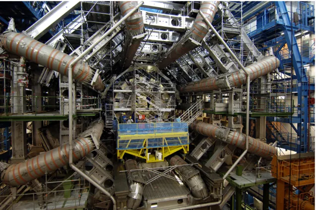
Figure 1.5: A view of the cavern where the ATLAS detector is being constructed. The eight toroid magnets can be seen as well as the central part of the calorimeter, which is installed into its position within the toroids. The picture was taken in December 2005 [10].

The status of the construction of the ATLAS detector at the beginning of 2006 can be seen from fig. 1.5.

1.4 Pixel detector

1.4.1 Layout

The Pixel detector [23] is a silicon detector consisting of 1744 rectangular modules, each of which covers a total sensitive area of 16.4 × 60.8 mm

²

. Each module carries 47232 pixels of size 50 × 400 µm

²

. This gives a 2-dimensional position measurement of charged particles within the plane of the module.

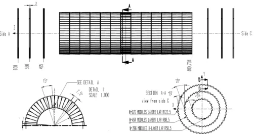
The layout of the Pixel detector is depicted in fig. 1.6. The detector is of cylindrical shape and is separated into a central barrel part and two endcaps. With dimensions of 130 cm in length and 38 cm in diameter, it covers a pseudorapidity range of |η| < 2.5.

The barrel consists of 3 cylindrical layers of modules with radii of 5.05, 8.85 and 12.25 cm.

These layers are built of 22, 38 and 52 so-called staves, respectively, each holding 13 mod-

ules. Thus, a total of 1456 modules compose the barrel part of the detector. The staves

are inclined by 20

^◦

with respect to the radial direction from the beamline to create an

overlap between adjacent modules (turbine arrangement). Additionally, the modules on

(13)

Chapter 1. Introduction 7

Figure 1.6: Geometry of the ATLAS Pixel detector. The sketch shows the overlap in the modules on one endcap disk, as well as the turbine-arrangement of the barrel staves, which in turn have the individual modules mounted in a shingled-stave layout. Gaps between modules are thus avoided. Dimensions are given in mm [24].

one stave are arranged in the so-called shingled stave layout to create an overlap in the global ˆ z-direction

⁴

. The long sides of the modules are oriented parallel to the beamline as well as to the long side of each individual pixel.

Each of the two endcaps has three discs, which have the modules mounted radially to the beamline, with their normal axis parallel to the beam. A disc is comprised of 8 sectors with 6 pixel modules each. This adds up to 2 × 144 modules on the endcap discs. When the pixel detector is fully built up, it will look like portrayed in fig. 1.7.

1.4.2 Principle of operation

In semiconductor particle detectors, p- and n-doped semiconductors are brought together to form a p-n junction [25]. The mobile charge carriers diffuse into the junction and recombine, leaving the fixed donor and acceptor atoms behind as spatial charges. This creates a depletion region free of mobile charge carriers and an intrinsic electric field which counterbalances the diffusion of mobile charge carriers into the depletion region.

In particle detectors, an additional external reverse bias voltage is applied to deplete the bulk as much as possible. Electron-hole pairs created by incident charged particles are separated by the electric field in this region and drift towards the electrodes. This charge is then collected and read out usually on one side of the detector. In pixel detectors, the two- dimensional separation of the readout pads makes it possible to have a two-dimensional position measurement.

The ATLAS Pixel modules are silicon sensors with n

⁺

-pixel implants on an n-type bulk.

The back contact is p-type (see fig. 1.8). The depletion region thus extends from the p-n junction at the backside. In the beginning, the reverse bias voltage must therefore be high

4for definition of coordinate systems see section 1.6

(14)

8 Chapter 1. Introduction

Figure 1.7: Raytraced image of the Pixel detector with an intersection cut away. One can clearly see the three discs of one endcap and the three barrel layers residing in the support frame [10].

enough so that the sensor is fully depleted. This is because the depletion region needs to reach the pixel implants so that any created charge can drift there to be read out.

The n

⁺

-on-n-design is chosen deliberately, because it is known that the long period of operation in extremely intense radiation will lower the impurity concentration and finally even type-invert the bulk to be effectively p-type. After a few months in the ATLAS detector, radiation damage will turn the bulk into effective p-type and the depletion zone will extend from the n

⁺

pads, making the detector usable even when it is not fully depleted.

However, with increasing radiation damage, more and more bias voltage will be needed to keep the depletion region large. The required bias voltage will range from about 150 V at the beginning up to 600 V after ten years of operation, which is the maximum depletion voltage possible for the sensor. Additionally, the silicon used is enriched with oxygen, which makes it more radiation hard.

The 250 µm thick silicon wafers are read out by 16 front-end (FE) chips. The chips provide 2880 channels each, which are bump-bonded with lead or indium solder bumps directly to the corresponding pixel on the silicon wafer (so-called flip-chip assembly). A Pixel module has a total of 144 × 320 = 46080 readout channels. Therefore, due to the necessary gap between adjacent FE chips, some of the 47232 pixels have to be grouped together on one readout channel. These form the so-called long pixels and ganged pixels. During track reconstruction, this irregular geometry due to fabrication necessities must be taken into account. A detailed sketch of this interchip region is shown in fig. 1.9.

The FE chips perform amplification, leakage current subtraction, signal shaping and

threshold discrimination and finally output the time-over-threshold (ToT) together with

a timestamp. On the other side of the detector substrate, the module control chip (MCC)

performs signal collection, multiplexing and optical data transmission to the readout sys-

tem.

(15)

Chapter 1. Introduction 9

Figure 1.8: Principle of operation of a pixel detector: electron/hole pairs generated by an ionizing particle are accelerated towards the electrodes. The signal is collected and read out at the n

⁺

pads. [26]

Figure 1.9: The interchip region between adjacent FE chips on a Pixel module [27, 28].

The gap in the pixel columns is covered by enlarged pixels, the so-called long pixels. In

the pixel rows, two pixels at a time are connected (ganged) to be read out together by one

channel of the FE chip.

(16)

10 Chapter 1. Introduction

Figure 1.10: Pixel module geometry. The cross-section of a module illustrates the attach- ment of the readout electronics on both sides of the sensor. Each module has a “pigtail”

which connects to the readout cables. [29]

1.5 Non-track-based alignment

For every position-sensitive detector in high energy physics it is essential that the position of each element be known very well to meet the detector performance requirement. The process of determining the true positions of the active elements of a detector is called alignment. For ATLAS, a three-stage strategy is foreseen: First, the detector parts will be built with as high as-built precision as possible and various geometrical quantities will subsequently be monitored (by optical means, mounting robot logfiles etc.). Second, some of the support structures will be monitored during running, for example with frequency scanning interferometry or other optical means, to detect movements and thermal distor- tions of bigger detector parts. Third, an accurate determination of geometrical positions will be performed using the particle tracks which traverse the detector themselves. The positions determined during alignment will be fed into the geometry database of the detec- tor and will later be available for track reconstruction; no actual movement of the detector parts is done. Alignment based on tracks will be the topic of the next chapters of this thesis.

The expected precision of the various methods and the precision required to meet the standards given by the Inner Detector technical design report (TDR) [20] can be seen in table 1.1. The precision numbers are based on the requirement that any misalignment of the inner detector parts must not degrade the reconstructed track parameters by more than 20%. However, to exploit the full precision that ATLAS is capable of, for example in order to measure the W mass with a resolution of 15 MeV, much more ambitious requirements must be fulfilled. It is estimated that in this case, the alignment precision for the sensitive pixel coordinate x has to be as good as 1 µm, which is significantly better than the intrinsic resolution of the detector.

The difference in the initial positioning precision between barrel and endcap modules comes

(17)

Chapter 1. Introduction 11 Pixel alignment precision

Pixel barrel Pixel endcap local coordinate required as-built required as-built

x 7 µm 50 µm 7 µm 4.6 µm

y 20 µm 20 µm 20 µm 4.7 µm

z 10 µm 50 µm 100 µm 12.7 µm

Table 1.1: Comparison of required alignment precision for Pixel modules as given by [20]

with the initial as-built precision from the survey [30].

from the existence of a very precise optical survey for the endcap. However, the survey can only measure module-to-module positions and therefore the absolute position in space of the endcaps is not known to the precision given in the table. For the barrel, survey information is not completely available, so that the initial precision basically depends on the mounting precision of the modules on the support structures.

The only method capable of improving the present precision for each individual module, and thus of fulfilling the strict requirements, is track-based alignment, which will be the topic of the next chapter.

1.6 Coordinate conventions

Within this thesis, two of the ATLAS coordinate systems are used [31]:

The global coordinate system is called the tracking frame. It is a right-handed three-

dimensional orthogonal coordinate system whose z-axis is parallel to the direction of the magnetic field in the inner detector. The origin lies at the nominal interaction point, and the x-axis points to the center of the LHC ring. We will denote coordinates within this frame with (ˆ x, ˆ y, ˆ z). Directions are usually given using the angles θ, which is the deflection with respect to the ˆ z-axis, and φ, which is the angle around the ˆ z-axis starting from ˆ x.

It is worthy to note that in collider experiments, the pseudorapidity η is often used as a variable to describe kinematic quantities. For relativistic particles the pseudorapidity is a good approximation of the true rapidity; the two quantities are identical for massless particles. The pseudorapidity is defined as

η = − ln tan θ

2 (1.1)

and often given instead of θ, because the density of particles produced in hadron collisions is known to be approximately uniform in η.

The local coordinate system of each module (x, y, z) is a unique system for each detector

module. For silicon modules, it lies in the corresponding plane of the detector with the

origin at the center of the module. The x-axis runs in the direction of the short coordinate

or across the strips, the y-axis runs in the direction of the long coordinate or along the

strips and the z-axis is perpendicular to the surface and oriented away from the interaction

point. In the following, rotations around these local axes will be denoted with (α, β, γ ).

(18)

Chapter 2

Track-based alignment

2.1 Alignment based on residuals

As outlined in the introduction, another method in addition to the survey of the detector system is needed to achieve the necessary alignment accuracy. To reach the desired goal, the direct use of tracks traversing the detector during operation achieves the highest precision of any method available. All track-based alignment methods are based on the minimization of residual distributions. The residual is hereby defined as “the distance”

between a track and its associated hit on a module surface.

The reconstructed track is the estimate of the true particle trajectory going through the tracking detector and plays a crucial role in all track-based alignment approaches. The ATLAS tracking detector is designed such that in general a charged particle leaves more than enough hits on the detector to constrain the set of equations necessary to describe a particle trajectory. On average, this will be 3 hits in the Pixel detector, 8 hits in the SCT and about 30 hits in the TRT. A helical track model for a charged particle traveling through a magnetic field needs five track parameters. In this way, it is ensured that under normal circumstances a statistical fit with error estimates can be performed. In the tracking software of a detector, two steps must be performed to reconstruct tracks from the many detector hits in one event. First, pattern recognition flags certain hits from the sample as belonging to one common particle trajectory. Then the actual track fitting algorithm takes over and estimates the optimal parameters for the assumed tracking model to fit the observed hit coordinates.

Over many tracks, the distribution of hits on a detector module will be roughly uniform.

The distribution of the residuals for a perfectly aligned module is then centered around zero with a gaussian shape. The shape is due to the acceptance for an individual detector element or a cluster to give a signal, which is dependent on the actual charge deposition position of the incident particle. A clustered hit arises if the path of a particle traversing the detector material is long enough so that the generated charge fires more than one readout channel. The position of the particle hit is then determined by taking into account position and charge information from these neighboring channels. Moreover, track fitting includes hits closer to the fitted particle trajectory more often than hits further away, which also contributes to the gaussian shape.

12

(19)

Chapter 2. Track-based alignment 13 If the detector module is not centered at its nominal position, then the residual distribu- tions will be shifted away from zero (c.f. fig. 2.1). In general, track based alignment relies on the minimization of residual distributions for some or all degrees of freedom of each detector module.

residual

# o f h its

reconstructed track real track

Figure 2.1: Four layers of modules, one of which is shifted away from its nominal position.

The real positions (shown in grey) are not known, thus the reconstructed track uses the nominal position (dashed) which degrades the fit quality. The residual distribution of this layer will be biased to one side. This is the basis for track-based alignment.

In the next section, the mathematical background of the used alignment approach will be presented.

2.2 Algebraic derivation of the χ

²

-minimization algorithm

The proposed approach is a linearized χ

²

-minimization which treats every module inde- pendently (so-called local approach), as it was used e. g. for the BABAR SVT detector [32]. It is described in detail in [33]. Here the major formalism will be presented in brief outline.

Having the vector of all residuals for a given track i, ~ r

i

= ~ r

i

(~a, ~ π

i

), the following χ

²

-function

is defined:

(20)

14 Chapter 2. Track-based alignment

χ

²

(~a, ~ π

₁

, . . . , ~ π

_m

) =

m

X

i ∈ tracks

~

r

_i^T

(~a, ~ π

_i

) · V

_i⁻¹

· ~ r

_i

(~a, ~ π

_i

). (2.1) Here, ~ r

i

(~a, ~ π

i

) depends on the alignment parameters ~a and the track parameters ~ π

i

. ~a are all alignment parameters of all modules that have hits on one of the tracks. ~ π

_i

is the vector of track parameters for track i. This can be e. g. 4 parameters for a straight line track model or 5 parameters for a helical track model. m is the total number of tracks used for the alignment. V

_i

is the covariance matrix of the residuals for track i.

It is noteworthy that r

_i

has two entries per traversed module for both SCT and Pixel modules: SCT modules have two wafer sides and therefore in general two hits per particle track, which are one-dimensional measurements. Pixel modules have one hit, which is a two-dimensional measurement, and therefore two residuals per hit on a module.

For a perfectly aligned detector, it is assumed that a minimal χ

²

is reached:

dχ

²

(~a)

d~a = ~ 0, (2.2)

with the derivative with respect to the alignment parameters defined as:

d d~a ≡







d da1

.. .

d dan







. (2.3)

Here, n is the total number of modules times the number of degrees of freedom for each module.

To solve equation 2.2, the left side is expanded in a linear Taylor expansion:

dχ

²

(~a)

d~a ≈ dχ

²

(~a) d~a

_~_a=~_a

0

+ d

²

χ

²

(~a) d~a

²

_~_a=~_a

0

∆~a. (2.4)

The expansion point a

0

is the vector of initial alignment parameters and (~a − ~a

0

) is abbreviated as ∆~a. Inserting the definition of χ

²

(2.1) yields:

dχ

²

(~a)

d~a = ~ 0 =

^X

tracks

d d~a

~ r

iT

(~a)V

_i⁻¹

~ r

i

(~a)

_~_a=~_a

0

+

^X

tracks

d

²

d~a

²

~ r

iT

(~a)V

_i⁻¹

~ r

i

(~a)

_~_a=~_a

0

∆~a =

= . . . =

^X

tracks

d~ r

_i

(~a) d~a

0

2V

_i⁻¹

~ r

_i

(~a

₀

) +

^X

tracks

d~ r

_i

(~a) d~a

0

2V

_i⁻¹

d~ r

_i

(~a) d~a

0

T!

∆ ~a (2.5)

Here,

^P_tracks

denotes the sum over all tracks

^P^m_i _∈ _tracks

, and

_d~^d_a

0

is the derivative eval- uated at a

₀

:

_d~^d_a

~a=~a0

. Since a linear approximation is done, all terms of the form

^d²_d~^~^r_aⁱ^(~2^a) 0

were neglected during the derivation of (2.5).

(21)

Chapter 2. Track-based alignment 15 The derivative of the vector of residuals with respect to the vector of alignment parameters is defined as:

d~ r d~a ≡







dr1

da1

dr2

da1

. . .

dr1

da2

dr2

da2

. . . .. . .. . . ..







. (2.6)

The formal solution to 2.5 is:

∆ ~a = −

^X

tracks

d~ r

i

(~a) d~a

₀

· V

_i⁻¹

· d~ r

i

(~a) d~a

₀

T!−1

·

^X

tracks

d~ r

i

(~a) d~a

₀

· V

_i⁻¹

· ~ r

i

(~a

0

)

!

. (2.7)

Thus, the vector of all alignment parameters ∆~a can be calculated using the residuals ~ r

i

(~a

0

) on all detector surfaces, their derivatives

^d~^r_d~ⁱ_a^(~^a)

0

with respect to all alignment parameters and the covariance matrices of the measurements V

_i⁻¹

.

There are several approaches to calculate the solution:

One approach, called the global χ

²

-approach [34], tries to directly invert the large matrix appearing as the first factor in (2.7). This can become quite complicated, as the whole silicon part of the inner detector has 1744 Pixel modules plus 4088 SCT modules, giving a total number of degrees of freedom of (1744 + 4088) × 6 = 34992. A single matrix of dimension 34992 ×34992 in double precision needs 4.5 Gigabytes in memory. Additionally, the inversion of this matrix is numerically challenging. How to do this is being investigated with special methods on a dedicated computer cluster.

The local χ

²

-approach tries to circumvent these problems by making some assumptions

about the matrix elements. The big matrices are broken up into 6 × 6 block diagonal matrices, by [33]:

• assuming that the correlation between different modules is small, i. e. no contribution from the derivative of r with respect to track parameters:

dr

i k

(~a

k

, ~ π

i

)

d~a

_k

= ∂r

i k

(~a

k

, ~ π

i

)

∂~a

_k

+ d~ π

i

d~a

_k

∂r

i k

(~a

k

, ~ π

i

)

∂~ π

i

| {z }

≈0

(2.8)

Here k is an index which counts the different modules.

To have this, the track parameters must be unbiased, i. e. the hit which is treated at the moment has to be removed from the track fit to make the fit independent of it.

• ignoring the dependence of the residual on the alignment parameters of other mod- ules, i. e.

dr

i k

(~a

k

, ~ π

i

) d~a

_l

= 0

!

∀ k 6= l. (2.9)

This can be justified if the error of the common track, which is the source of module- to-module correlations, is small compared to the error of a measurement on the module. Later on, we will test this assumption by determining if

σ

_{T rack}

σ

_Hit

2

< 1. (2.10)

(22)

16 Chapter 2. Track-based alignment

• assuming that the covariance matrix is diagonal, i. e. the measurements on different detector surfaces are uncorrelated. This is in general not true because of multiple coulomb scattering (MCS). To suppress these contributions, we seek to use only high-momentum tracks which have negligible MCS contributions. For example, a particle of 10 GeV/c momentum would have a RMS of the deflection angle due to MCS of 0.054 mrad after passing through 250 µm of silicon. For module layers which are 4 cm away from each other, this would mean an additional position error of 2.2 µm on the next layer, which is well below the position resolution of the silicon detectors. Thus, 10 GeV/c is reasonable as the minimum momentum when selecting appropriate tracks.

Making these assumptions, formula 2.5 reduces to a 6 × 6 block-diagonal form and can be solved independently for each module:

∆~a

_k

= −

^X

tracks

1 σ

²_{i k}

∂r

_{i k}

(~a

_k

)

∂~a

_k₀

∂r

_{i k}

(~a

_k

)

∂~a

_k₀

T!−1

·

^X

tracks

1 σ

²_{i k}

∂r

_{i k}

(~a

_k

)

∂~a

_k₀

r

_{i k}

(~a

_k₀

)

!

. (2.11) The covariance matrix for the vector of alignment parameters is then given by [35]:

h

σ

²_aⁱ

= 2 ∂

²

χ

²

∂a

²₀

!−1

≈

^X

tracks

1 σ

²_i

∂r

i

(~a) d~a

₀

∂r

i

(~a) d~a

₀

T!−1

, (2.12)

and thus the error of the alignment parameters is:

σ

a j

=

^q

σ

_{a jj}²

. (2.13)

2.3 Iterations

It is clear that the solution to equation (2.11) will not initially be the best possible solution because of the neglecting of correlations. Therefore, the algorithm needs iterations to converge to a stable solution.

The first iteration leads to an alignment solution which already gives better track fits because of the improved positions of the modules. After redoing the track fitting with the better detector geometry, the alignment procedure is repeated to give a further improved alignment solution than in the first iteration. This procedure is performed again until a final convergence criterium is met.

Thus, by iterating over a track sample several times and repeating track reconstruction, the neglected correlations between different modules are taken into account implicitly.

Since the alignment algorithm just minimizes residuals, its solution is not necessarily

unique: If the equation system (2.7) is degenerate, the algorithm will converge to a solu-

tion, which might not be the perfect alignment solution. Therefore another crucial point of

the local approach is the appropriate selection of track samples and additional constraints

– e. g. vertex or momentum constraints – to remove the multiple solutions to the alignment

problem and make the solution unique.

(23)

Chapter 3

Prototype simulation with ROOT

3.1 ROOT software

ROOT is a C

⁺⁺

-based program package for data analysis in science, especially high energy physics. It was and still is developed at CERN, but may be used freely by the entire scientific community. Its capabilities range from histogramming to mathematical analysis, including powerful statistics and fit functionality, to geometry simulation and visualization.

The full documentation and code can be found at the ROOT webpage at CERN [36, 37].

In this diploma thesis, the ROOT package was used to write a small simulation program to investigate the functioning and features of the local alignment approach for the Pixel detector.

3.2 Geometry and tracking

With ROOT it is possible to simulate a simple geometry independent of the ATLAS detector software framework and to study the performance of our approach in a clean and controllable environment. The geometry was reduced to one cuboid Pixel module having the dimensions of a real Pixel module, which are 16.4 mm × 60.8 mm × 0.3 mm.

Then straight line tracks were created, originating from a common vertex and equally distributed across a certain solid angle, i.e. equally distributed in φ and cos θ (c.f. fig. 3.1).

The coordinate system was chosen to be compliant with the ATLAS coordinate conven- tions, i. e. we use the global and local coordinate frames defined in section 1.6.

To mimic the setup of an ATLAS Pixel module, the positions were chosen as follows:

All tracks originate from the global origin and the Pixel module was placed at the global coordinates (17.27 mm, 0, 47.45 mm). This position corresponds to a barrel module of the innermost Pixel layer sitting at η = 0.

Then tracks were propagated through the geometry by ROOT’s tracking capabilities. The intersection point of the track with the surface of the module was taken to calculate the pixel which was hit by the track. Thus, neither an error from a track fit nor the effect of pixel clusters were simulated.

17

(24)

18 Chapter 3. Prototype simulation with ROOT

Figure 3.1: Drawing of the simulated Pixel module. The division into 16 parts illustrates the sections read out by individual FE chips. Some straight line tracks originating from a common vertex cross the module.

3.3 Implementation of the algorithm

From chapter 2 it can be seen that the simulation must calculate the following quantities:

residuals, residual errors and residual derivatives with respect to the alignment parameters.

3.3.1 Choice of residuals In-plane residuals

The in-plane residuals are defined as the distance between the track and its associated hits within the detector plane. Because a Pixel module performs two independent mea- surements of two coordinates, a single hit results in two residuals in the local x- and y-directions. Within the simulation, residuals are calculated by the signed distances of the pixel-center in x, y and the impact point of the track:

r

_x

r

_y

!

in−plane

= x

impact point

− x

pixel center

y

impact point

− y

pixel center

!

(3.1)

The distributions of in-plane residuals are uniform with a total width equal to the corre- sponding pixel x- and y-size (not shown).

DOCA-residuals

The Distance Of Closest Approach-residuals (DOCA) are defined as the shortest distance

in space between the straight line track and a straight line corresponding to one readout-

coordinate of the detector (see [33]). Because a Pixel module has no readout-strips, a

two-dimensional grid of readout-strips crossing each other in every pixelcenter is artificially

formed, as shown in fig. 3.2. Thus the same formalism which is already in place for ATLAS

SCT-modules can be used while retaining the two-dimensional readout for pixels.

(25)

Chapter 3. Prototype simulation with ROOT 19

virtual readout-strips

in-plane residual

pixelcenter DOCA residual

particle track impact point

particle track

in-plane residual

DOCA residual δ

Figure 3.2: The definition of distance of closest approach residuals for Pixel modules.

The dashed lines symbolize the classical in-plane residuals, the red lines denote the DOCA residual. On the right hand side, the y-residuals are shown in a y-z-projection.

The DOCA-residual is calculated as follows: from the two straight-line equations describ- ing the track

~ x =







a

₁

a

2

a

₃







+ λ







b

₁

b

2

b

₃







(3.2)

and one readout coordinate of a pixel

~ x

⁰

=







c

1

c

₂

c

₃







+ κ







d

1

d

₂

d

₃







(3.3)

the signed shortest distance can be computed via determinants [38]:

r

_DOCA

=

a

₁

− c

₁

a

₂

− c

₂

a

₃

− c

₃

b

1

b

2

b

3

d

₁

d

₂

d

₃

v

u u t

b

1

b

2

d

₁

d

₂

2

+

b

2

b

3

d

₂

d

₃

2

+

b

3

b

1

d

₃

d

₁

2

(3.4)

If calculated in the local coordinate frame of the module, the two readout-strips receive direction vectors of d ~ = (0, 1, 0)

^T

for x-strips (where the strip is parallel to the y-axis and the measurement is sensitive to the x-coordinate) and d ~ = (1, 0, 0)

^T

for y-strips (vice- versa). In both cases, the starting point ~ c will be the pixel center.

DOCA residuals have a uniform distribution with smeared edges because tracks crossing

non-perpendicularly have a smaller DOCA residual compared to in-plane residual, as

shown in fig. 3.3.

(26)

20 Chapter 3. Prototype simulation with ROOT

Entries 1000000

Mean 0.004548

RMS 13.9

Underflow 0

Overflow 0

µm]

x [

r

-50 0 50

3 entries/10

0 2 4 6 8 10 12 14 16 18 20 22

Entries 1000000

Mean 0.004548

RMS 13.9

Underflow 0

Overflow 0

x-coordinate

rDOCA _Entries _1000000

Mean 0.1334

RMS 110.1

Underflow 0

Overflow 0

µm]

y [

r

-400 -200 0 200 400

3 entries/10

0 2 4 6 8 10 12 14 16 18 20 22

Entries 1000000

Mean 0.1334

RMS 110.1

Underflow 0

Overflow 0

y-coordinate

rDOCA

Figure 3.3: Distributions of the DOCA residuals

”Single” residuals

If one takes the distance to the center of the pixel as the (single) quantity to minimise, the two residual definitions take the form:

r

in−plane

=

^q

r

²_x

+ r

²_y

(3.5)

r

DOCA

=







b

1

b

₂

b

3







×







r

x

r

_y

0













b

1

b

₂

b

3







(3.6)

It was found that these residual definitions yield poor results compared to the traditional x- and y-residuals. This is because the two initially independent measurements are combined with one common accuracy. It is found that sensitivity is transferred from the sensitive x-coordinate to the less sensitive y-coordinate. This leads to the somewhat counterintuitive result that the x-coordinate is less sensitive than the y-coordinate.

This can be understood by looking at the error of the in-plane residuals:

σ

_r

=

s

∂r

∂x σ

_x 2

+ ∂r

∂y σ

_y 2

=

s

r

x

r σ

_x 2

+ r

y

r σ

_y 2

(3.7)

The errors for the x- and y-coordinate are only used in combination. Since large y-

residuals are much more probable due to the large aspect ratio of the rectangular pixel,

the y-coordinate dominates the error most of the time. Another result of this resolution

loss are the peculiar derivatives of this single residual: the derivatives with respect to x

(27)

Chapter 3. Prototype simulation with ROOT 21 are often close to zero, a clear sign that the x-coordinate is not sensitive to alignment corrections (see section 3.3.4).

Due to this shortcomings, “single” residuals are not discussed any further in this thesis.

3.3.2 Gaussian versus non-gaussian input

Due to track fitting uncertainties and clustering effects, which are missing in the ROOT simulation, the distributions of the residuals in the Athena-implementation of the align- ment approach will not be uniform but instead will be roughly gaussian. The algorithm performs equally well under these conditions. This is due to the central limit theorem [38]: The sum of many random variables of the same distribution will have a gaussian distribution, regardless of the shape of the random variable’s distribution. Therefore the input distribution of the residuals becomes irrelevant since χ

²

is computed as their sum.

Of course the error estimate must be correct for both types of input. The validation of our simulation with gaussian-shaped input residuals is shown in [33].

3.3.3 Residual errors

The errors of the two in-plane residuals were taken to be the RMS of a uniform distribution, which is

σ = strip pitch

√ 12 . (3.8)

For the two errors of the DOCA-residuals, error propagation yields:

r

_DOCA

= r

_in−plane

· sinδ (3.9)

σ (r

DOCA

) =

s

∂r

_DOCA

∂x

σ

_x²

+

∂r

_DOCA

∂y

σ

²_y

+

∂r

_DOCA

∂δ

σ

_δ²

, (3.10) where δ is the angle between the detector strip and the track projection on a plane perpendicular to the detector strip, as depicted in fig. 3.2.

The first term of (3.10) is zero for y-residuals, the second for x-residuals. The third term was taken to be zero, because in this simulation with perfect tracks, the error of δ is zero.

Later on, the third term will denote the track fitting error.

It was verified that both the usage of partial derivatives and the direct calculation of sin δ give the same results for the DOCA error.

3.3.4 Calculation of derivatives

The calculation of derivatives with respect to the six alignment parameters was performed numerically using the two-sided difference quotient:

∂r

∂a

i

= r(a

_i

+ h

_i

) − r(a

_i

− h

_i

) 2h

i

(3.11)

(28)

22 Chapter 3. Prototype simulation with ROOT In the simulation, the module was displaced by a small distance ±h

_i

and the two residuals were calculated for each coordinate and each of the six alignment parameters. Distribu- tions of the residual derivatives can be seen in figs. 3.4 and 3.5. Additionally, figs. A.1 and A.2 show these distributions in the case of in-plane residuals.

Many features of these derivative distributions for a barrel module have simple explana- tions:

•

^∂r_∂x^x

would be exactly one for in-plane residuals. Since the tracks cross at an angle, the DOCA residuals change less than in-plane residuals when moving in x. Due to the 20

^◦

tilt angle,

^∂r_∂x^x

scatters around cos −20

^◦

= 0.94 (fig. 3.4a).

•

^∂r_∂y^x

must be zero, since x-strips run parallel to the local y-axis (fig. 3.4b).

•

^∂r_∂z^x

would be zero for tracks crossing the module at right angles. Since this is not the case, the module acquires some sensitivity in z, i. e. has non-zero derivatives.

The incident angle in the x-z-projection scatters around 20

^◦

and thus the derivative distribution is symmetric around sin −20

^◦

= −0.34 (fig. 3.4c).

• For the angles, large derivatives occur when the lever arm for rotations around the axis is large, i. e. the module has its long coordinate there. Here one has to keep in mind that the rotation is always with respect to the center of the Pixel module.

Large derivatives occur e. g. for the long strips parallel to y when rotated around x, i.e.

^∂r_∂α^x

(fig. 3.4d).

• The rotations around y, such as

^∂r_∂β^x

, contribute smaller values than rotations around x since the module is not as wide in the x-direction than it is in the y-direction (fig. 3.4e).

• Large derivatives occur also for rotations around z, i.e.

^∂r_∂γ^x

. The crossing angle in the y-z-plane is symmetric around zero, and so is

^∂r_∂γ^x

(fig. 3.4f).

•

^∂r_∂x^y

is zero, similarly to

^∂r_∂y^x

(fig. 3.5a).

•

^∂r_∂y^y

would be exactly one for in-plane residuals. For DOCA-residuals,

^∂r_∂y^y

is deter- mined by the length of the module in y and receives contributions from cos 0

^◦

= 1 down to cos 59.0

^◦

= 0.52 (fig. 3.5b).

•

^∂r_∂z^y

would be zero for tracks crossing the module at right angles. Again, the symmet- ric distribution of crossing angles in the y-z-plane makes this distribution symmetric around zero, with a maximum of cos 32.6

^◦

= 0.84 (fig. 3.5c).

•

^∂r_∂α^y

is large, since strips in x-direction on the outer sides of the module contribute large values when rotated around x (fig. 3.5d).

•

^∂r_∂γ^y

is not symmetric – in contrast to

^∂r_∂γ^x

– due to the tilt angle in the x-z-plane (fig. 3.5f).

As a consequence one can say that the observed distributions lie well within the expec-

tations. Later on, they will be compared with the results obtained from the Athena

implementation.

(29)

Chapter 3. Prototype simulation with ROOT 23 The absolute value of the derivatives is a direct measure of the sensitivity track-based alignment has with respect to this degree of freedom, since it indicates the change of the residual distribution when moving along this degree of freedom. It can be seen from the derivative distributions that x-residuals constrain the x-coordinate and the rotations fairly well. The largest derivatives and therefore the highest sensitivity are with respect to γ , since a rotation of the module within its plane always changes the residual distribu- tion considerably. The z-coordinate acquires some sensitivity due to the tilt angle of the module, which leads to a change of x-residuals when moving along the local z-direction.

For residuals in the y-direction, the converse is true: These residuals are sensitive to shifts in y, but not in x. Sensitivity in z comes into play via the varying incident angle over the whole length of the module. The rotations are also well constrained, due to the large lever arms when rotating around the module center.

The advantage of Pixel modules from the point of view of the alignment is that the use of both residuals constrains both x and y well, with x being more sensitive than y due to the smaller error of the x-residual. From the simulation it is concluded that the combination of x- and y-residuals and the special barrel geometry chosen (tilt angle in x and central position in y) should constrain all six degrees of freedom well.

3.3.5 χ

²

minimization

The calculated residuals, residual errors and derivatives were fed into equation 2.11 and the alignment parameters and their errors were calculated. Figure 3.6 shows the alignment results using 1000 hits on the module and repeating the whole procedure 1000 times. In Appendix A, the corresponding plot is shown using in-plane residuals (fig. A.3)

The pull distributions, i. e. the difference between the true and calculated values normalized by the error

pull

_a_i

= a

_i,true

− a

i,calculated

σ

ai

(3.12) are also shown (figs. 3.7, A.4). Pull distributions allow one to check whether the calculated values are correct (pulls should be centered around zero) and whether the error estimates are consistent (pulls should have a width of 1).

3.4 Performance of the algorithm and results

The algorithm was tested as shown above with no misalignment (nominal alignment).

In addition, runs with a misaligned module were performed. For this, alignment parame- ters and the corresponding pulls can be seen in figs. 3.8 and 3.9. For comparison, results with in-plane residuals are shown in appendix A (figs. A.5 and A.6). In both cases, the module was shifted by ∆x = 12 µm, ∆y = 25 µm, ∆z = −30 µm and rotated around γ by -2 mrad, then around β by 5 mrad and finally around α by 5 mrad.

Iterative local χ 2 alignment algorithm for the ATLAS Pixel detector