Kalman Style Alignment Approach for the ATLAS SCT and Pixel detectors

(1)

SCT and Pixel detectors

Diploma Thesis

supervised by Prof. Dr. S. Bethke

Manuel Kayl Physik-Department Technische Universit¨at M¨unchen

and

Max-Planck-Institut f¨ur Physik Werner Heisenberg Institut

Munich, January 8, 2007

(2)

Abstract

ATLAS is one of the four experiments at the Large Hadron Collider (LHC) currently under construction at CERN in Geneva, Switzerland. The main tracking device of ATLAS, the Inner Detector, consists of the Transition Radiation Tracker (TRT), the SemiConductor Tracker (SCT) and the Pixel detector.

An approach for the alignment of the SCT and Pixel detector modules with particle tracks is presented. All 5832 silicon detector modules are aligned. The presented Kalman style alignment approach (KASTRO) is an extension to the localχ² alignment approach and uses a standard recursive filter, the Kalman filter. The Kalman filter technique has never been used before for the alignment of a running experiment. KASTRO has been incorporated into the ATLAS software framework Athena and provides the most probable set of alignment parameters for each module individually. The alignment parameters are calculated recursively after each track and the current estimate of the module position and orientation is updated. Module-to-module correlations are taken into account immediately by performing a refit of the tracks on the updated detector geometry. The goal of KASTRO is to avoid the time consuming iterations the local χ² alignment approach intrinsically depends on.

A derivation of the mathematical concepts is presented. The achievable alignment accuracies were investigated within Athena based on Monte Carlo simulated tracks. Tests on nominal and misaligned geometry setups were performed.

(3)

Acknowledgements

First I want to thank my mother, my father and my grandmother for providing me the opportunity to study physics and write this thesis. Without their financial and emotional support this would not have been possible.

I want to thank Prof Bethke for introducing me to the field of high energy physics and for offering me the possibility to write my diploma thesis at the Max-Planck-Institut within the ATLAS collaboration.

My sincere thanks go to my three advisors Stefan Kluth, Richard Nisius and Jochen Schieck. From my first day at MPI they gave me the feeling of being a full member of our group. Their unceasing support has been the basis for my work. Thank you for investing so much time and for guiding my work always in the right direction.

My biggest thanks go to my two precursors, Roland and Tobias. Without their day-to-day support I would have been lost. I also want to thank Andrea, Nabil and Sophio for creating the pleasant atmosphere in our group making me never even think about regretting my choice to work at the MPI.

A special thank you goes to all the people from CERN supporting me and making me enjoy each stay in Geneva, especially to Andi Salzburger aka Edi Finger. Without their help Athena would still be a mystery for me. I also want to thank ”Mr Kalman” Rudi Fr¨uwirth for providing his expertise although working for a rivalry experiment.

Finally all my love goes out to my girlfriend Bettina and all my friends. Thank you for tolerating my bad moods and for making me remember that there is a life beyond physics.

iii

(6)

Overview

The Kalman style alignment approach (KASTRO) is presented in this thesis. KASTRO is a track-based alignment approach for the ATLAS Inner Detector which makes use of a standard recursive filter, the Kalman filter. The work is described in six chapters that are structured as follows:

• Chapter 1 – Introduction

The LHC and the general purpose detector ATLAS are described briefly among the physics goals of the project. The ATLAS SCT and Pixel detectors are explained in more detail. Basic concepts of detector alignment are presented.

• Chapter 2 – Kalman Style Alignment Approach (KASTRO)

A brief derivation of the localχ² alignment algorithm is given. The basic concepts of a Kalman filter are exemplified with the aid of a track fitter of the ATLAS experiment based on the Kalman filter technique. The mathematical backgrounds of the Kalman filter and their application to detector alignment are presented.

• Chapter 3 – Prototype Programme with ROOT

The feasibility of KASTRO is studied within a prototype programme in ROOT.

The calculation of the input quantities (residuals, residual derivatives and residual errors) for the approach is explained. Results on the performance of the approach are shown with nominal and misaligned geometry setups.

• Chapter 4 – Implementation of the Algorithm in Athena

The basic concepts of the ATLAS software framework Athena and of the implementation of the localχ² alignment approach into Athena are outlined. The modifications of the localχ² alignment approach, of the detector description and of the track fitter necessary to implement KASTRO into Athena are described. The input quantities of KASTRO are studied in detail.

• Chapter 5 – Validation and results

The performance of KASTRO is investigated for all modules of the SCT and Pixel detector. The achievable alignment accuracies are studied. Tests on nominal and misaligned geometry setup are performed. The results obtained with these test are discussed.

• Chapter 6 – Conclusions

The main points of the preceding chapters are summarised. Ongoing developments and unresolved issues are discussed alongside future plans.

iv

(7)

Introduction

1.1 Standard Model of particle physics

The Standard Model (SM) of particle physics consists of quantum field theories describing the fundamental matter particles and their interactions precisely. It has been successfully tested up to an energy scale ofO(200 GeV) [1, 2].

The fundamental matter particles possess spin ¹₂ and thus are fermions. These fundamental fermions exchange field quanta which mediate the forces between them. These field quanta are spin-1 particles, the gauge bosons. They arise from the requirement of local gauge invariance and are a manifestation of the symmetry group of the SM, SU_C(3)×SU_L(2)×U_Y(1).

The fundamental fermions are leptons and quarks. They are grouped into three genera- tions, each generation consisting of two quarks and two leptons. The interactions between the fermions belong to two different sectors. The strong interaction between quarks is described by Quantum Chromodynamics (QCD) based on the symmetry group SU_C(3).

The gauge bosons of QCD are the gluons. The electroweak interaction is described by the unification of Quantum Electrodynamics (QED) and the weak interaction based on the symmetry group SUL(2)×U_Y(1). The electroweak force is mediated by W^± and Z bosons as well as by photons.

A key feature of the SM is the mechanism of spontaneous symmetry breaking of the electroweak gauge group, the Higgs mechanism [3]. The Higgs mechanism gives an expla- nation for the different masses of the electroweak gauge bosons. It predicts the presence of a massive spin-0 boson, the Higgs boson. The Higgs boson is the only particle of the SM which has not yet been experimentally observed.

1.2 Large Hadron Collider

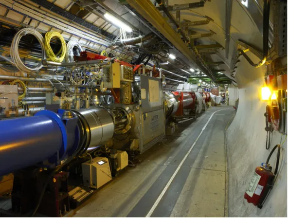
The Large Hadron Collider (LHC) [4, 5] is a circular particle accelerator which is currently under construction at CERN in Geneva, Switzerland. It will be integrated into the 27 km long tunnel which housed the Large Electron-Positron Collider (LEP) [6], in operation from 1989 until 2000.

1

(8)

2 Chapter 1. Introduction

Figure 1.1: A view of the LHC tunnel with previously installed components of the accelerator. [7]

Contrary to the e⁺e⁻ collider LEP, LHC operates by colliding two beams consisting of protons with an energy of 7 TeV energy providing a center of mass energy of 14 TeV [8].

Since protons are not elementary particles, only a fraction of the center of mass energy is carried by the colliding constituents. The maximum center of mass energy of a collision is expected to be about 5 TeV. The primary goal of LHC is to make an initial exploration of the 1 TeV scale. The construction is scheduled to be completed in late 2007.

The machine is also designed to produce collisions of heavy ions like lead to exploit the physics potential of nucleus-nucleus interactions at LHC energy scales.

The operation of the LHC is divided into two phases. First there will be a low luminosity run with an expected luminosity of 10³³cm⁻²s⁻¹. A high luminosity run will follow at a luminosity of 10³⁴cm⁻²s⁻¹ [9]. One proton bunch will consist of 11×10¹⁰ protons and the time between two collisions will be 25 ns. The total number of bunches that are simultaneously in the LHC ring will be 2808 at high luminosity. Per bunch crossing, about 20 hard interactions will take place. It is expected that roughly 1k tracks arise per bunch crossing leading to a number of 4×10¹⁰ tracks per second in a detector. A view of the LHC tunnel with previously installed components of the LHC machine is given in figure 1.1.

The LHC has four interaction points as shown in figure 1.2. Two of them are dedicated to the multipurpose experiments ATLAS (A Toroidal Lhc ApparatuS) [10] and CMS (Compact Muon Solenoid) [11]. The other two caverns are for the LHCb experiment

(9)

[12], focusing on b-physics, and the heavy ion experiment ALICE (A Large Ion Collider Experiment) [13].

Figure 1.2: Schematic view of the LHC ring with its four major experiment sites. [7]

1.3 ATLAS detector

The most important goals of the ATLAS physics programme are the following [14] :

• Exploration of electroweak symmetry breaking and the search for the Higgs boson. If the Higgs mechanism describes electroweak symmetry breaking correctly, the Higgs boson can be discovered in ATLAS. The lower limit on the mass of the Higgs boson from direct searches from LEP is 114.5 GeV [15].

• Discovery of new physics beyond the SM. Searches for new physics such as super- symmetry, extra space dimensions and dark matter candidates will be performed by the ATLAS group.

• Precise measurements of SM quantities, such as CP-violation in B meson decays or the mass of the W boson as well as mass and cross section of the top quark.

The general purpose detector ATLAS, shown in figure 1.3, is designed to make use of the full potential provided by the LHC. It has a onion-like structure consisting of:

(10)

Figure 1.3: Schematic view of the ATLAS detector and its components. [7]

• the muon spectrometer

• the calorimeter system

• the tracking devices

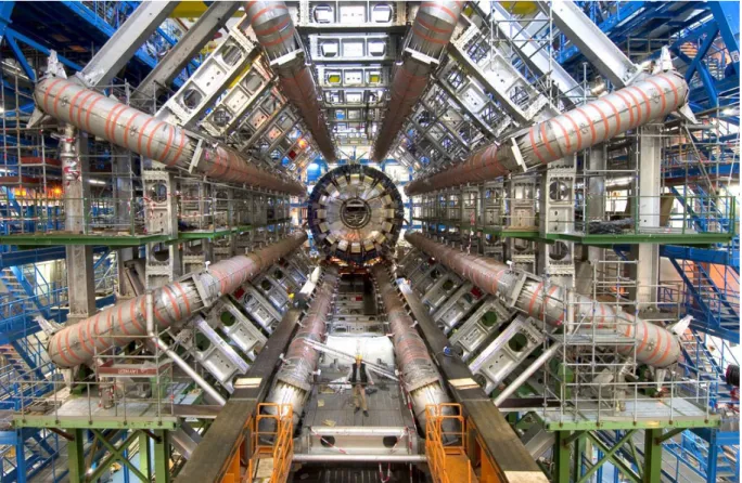
A very good muon identification and momentum measurement plays a key role in many interesting physical processes. The ATLAS muon spectrometer [16] composes most of the volume of ATLAS. The conceptual layout is based on the magnetic deflection of muon tracks in a system of superconducting toroidal air-core magnets [17, 18] providing a magnetic field of up to 4 T. The installed toroidal magnets are shown in figure 1.4.

The muon spectrometer consists of a barrel part and two endcaps. In the barrel region, tracks are measured in chambers arranged in three cylindrical layers around the beam axis.

In the endcap regions, the chambers are arranged in three layers as well, but are mounted perpendicularly to the beam line. The chambers used for the detection of muons are Monitored Drift Tubes (MDT) and Cathode Strip Chambers (CSC). Optical alignment systems have been developed to perform a survey of the chambers and thus fulfil the stringent requirements placed on positional accuracy.

The ATLAS calorimeter system consists of two separate calorimeter types, the hadronic calorimeter and the electromagnetic calorimeter (EMC). Particles crossing a calorimeter interact with its material and deposit quantities of energy which can be measured. The EMC covers a region of|η|<3.2¹, the barrel part of the hadronic calorimeter (TileCal)

1ηis the pseudorapidity, c.f. section 1.5

(11)

Figure 1.4: ATLAS detector under construction in the cavern. The eight toroidal barrel magnets can be seen. They were installed into ATLAS in October 2005. [7]

|η| < 1.7. The range 1.5 < |η| < 3.2 is covered by the hadronic endcap calorimeters (HEC). The extreme forward region 3.2 < |η| < 4.9 is covered by forward calorimeters (FCAL). All ATLAS calorimeters are sampling calorimeters, but they make use of different active and absorptive materials. The TileCal uses scintillating plastics as active material, whereas all other calorimeters use liquid argon. The absorber materials are iron (TileCal), lead (EMC) , copper (HEC and electromagnetic FCAL) and tungsten (hadronic FCAL) [19–21].

Inside the EMC, a solenoid magnet [22] provides a 2 T magnet field for the main tracking device, the Inner Detector [23, 24]. Even very high momentum particles curve significantly in this field so that their momentum can be determined.

1.4 Inner Detector

The ATLAS Inner Detector is designed to make high precision measurements of kinematic parameters of charged particles. The task of the Inner Detector is to reconstruct tracks and vertices in the proton collisions. Due to the high resolution provided, the displacement of secondary vertices can be determined. A three-dimensional cutaway view of the layout is shown in figure 1.5. The Inner Detector consists of three subdetectors:

• the Transition Radiation Tracker (TRT)

(12)

Figure 1.5: Three dimensional view of the Inner Detector consisting of TRT, SCT and Pixel detector. [7]

• the SemiConductor Tracker (SCT)

• the Pixel detector

Each subdetector provides full tracking coverage for a region of|η|<2.5.

The outermost component of the Inner Detector is the TRT [25]. It is a transition radiation tracker designed to operate at very high rates. The TRT consists of straw tubes and foils initiating the transition radiation. The barrel part consists of 50k straws and the endcaps together consist of 320k straws. A single straw has a diameter of 4 mm and a variable length of up to 150 cm. Each straw provides a spatial resolution of 170µm. The TRT is capable of identifying electrons by employing xenon as filling gas for the straws to detect transition radiation photons. The transition radiation photons which are produced in the radiator foils between the straws by the electrons can thus be detected.

The SCT and the Pixel detector together compose the silicon part of the Inner Detec- tor. Since this thesis is about the alignment of the silicon Inner Detector modules, these subdetectors are explained in more detail.

1.4.1 SCT

The SCT is made up of a barrel and two symmetric endcap trackers consisting of 4088 detector modules in total [26]. Different layouts exist for SCT barrel and endcap modules.

The barrel is made of 2112 barrel SCT modules arranged in four cylindrical layers parallel to the beam axis. The properties of the different barrel layers can be found in table 1.1.

A SCT barrel module consists of two rectangular detector surfaces which are about 12 cm long, 6 cm wide and 285 µm thick. They are glued back-to-back and rotated with a stereo angle of 40 mrad with respect to each other. The modules are mounted with a

(13)

tilt angle of 10 degrees. Each surface consists of two active quadratic silicon diodes of approximately (6×6) cm². The readout channels are 768 aluminium strips with a strip pitch of 80µm. The readout strips of one surface, the r-φside, are aligned parallel to the beam line, whereas the readout strips of the other surface, the stereo side, are rotated by 40 mrad with respect to the beam line.

SCT barrel configuration

Barrel Layer mean radius (cm) number of modules tilt angle (degrees)

0 30 384 10.0

1 37 480 10.0

2 44 576 10.0

3 51 672 10.0

Table 1.1: List of the mean radius, the number of modules and the tilt angles of the four SCT barrel layers [27].

Each endcap tracker consists of 988 endcap SCT modules which are mounted on nine discs placed perpendicular to the beam line [28]. The distance measured along the beam line to the interaction point is 83 cm for the closest disc and 277 cm for the farthest. The modules are arranged on up to 3 rings depending on the distance to the interaction point. The properties of the different endcap discs can be found in table 1.2. Three different kinds of endcap SCT modules exist depending on the position at which they are mounted on a particular ring: inner modules, middle modules and outer modules. All endcap modules are wedge-shaped. They consist of two detector surfaces, r-φ and stereo side, which are glued back-to-back and rotated with a stereo angle of 40 mrad with respect to each other.

Each surface has 768 readout strips emerging radially from the beam line. The strip pitch increases with radial distance and is between 55 µm and 95 µm. A SCT outer endcap module is shown in figure 1.6.

Figure 1.6: A SCT endcap module is shown. The readout strips run from left to right. [7]

(14)

8 Chapter 1. Introduction SCT endcap configuration

Disk # inner modules # middle modules # outer modules total

0 0 40 52 92

1 40 40 52 132

2 40 40 52 132

3 40 40 52 132

4 40 40 52 132

5 40 40 52 132

6 0 40 52 92

7 0 40 52 92

8 0 0 52 52

Table 1.2: List of number of module types mounted on the nine SCT endcap discs.[29]

1.4.2 Pixel

The Pixel detector consists of a barrel and two endcap trackers. The Pixel detector is composed of 1744 modules with a single design throughout the whole detector [30].

The Pixel barrel consists of 1456 modules arranged in three layers around the beam line.

The properties of the layers can be found in table 1.3. The dimensions of a single Pixel module are roughly 1.6 cm × 6.1 cm × 300 µm. Each module consists of 47232 pixels each covering an area of (50× 400)µm². The modules are mounted with a tilt angle of 20 degrees on the layers. A Pixel module is shown in figure 1.7.

Figure 1.7: A Pixel module with its readout electronics. [7]

Pixel barrel configuration

Barrel Layer mean radius (cm) number of modules tilt angle (degrees)

0 5.05 286 20.0

1 8.85 494 20.0

2 12.25 676 20.0

Table 1.3: List of the mean radius, the number of modules and the tilt angles of the three Pixel barrel layers [27].

One Pixel endcap is made up of three discs containing 48 modules each. The modules are mounted radially to the beam line. The distances of the discs from the interaction point are 45 cm, 58 cm and 65 cm.

(15)

1.4.3 Principle of operation

Silicon detector modules arep−njunction diodes. The diodes are operated at reverse bias by applying an additional high voltage [31]. The intrinsic electric field is amplified and a sensitive region depleted of mobile charge carriers is formed. A charged particle passing through the depletion zone produces electron-hole pairs along its path. Due to the electric field, the electron-hole pairs drift towards the electrodes. The number of electron-hole pairs is proportional to the energy loss of the charged particle. The signal produced is read out at one of the diodes.

The readout structures can either be strips providing a one dimensional measurement as in the case of the SCT modules or pads creating two dimensional measurements as is the case for the Pixel detector modules. The principle of operation for both module types is shown in figure 1.8. The bias voltage is about 150 V at the start of LHC operation in both cases and will increase during the operation time because of the irradiation of the modules.

Figure 1.8: Thep−njunction diodes with the p⁺ readout strips for the SCT are shown on the left. On the right side, a drawing of thep−n junction diodes and the two dimensional n⁺ readout pads of the Pixel detector is shown. [32]

For the SCT modules, the readout of the signal is binary, meaning that no pulse-height information is recorded for fired strips, but only the fact that they were above threshhold.

The spatial resolution of the SCT modules considering a 200 GeV muon is expected to be about 23µm [23]. It is mainly limited by the strip pitch and given by strip pitch√

12 .

For the Pixel modules, the time-over-threshhold (ToT) is recorded. The ToT provides additional information to the position measurement since the charge shared between fired pixels can be determined. A Pixel detector module is capable of measuring the impact parameter of a 200 GeV muon with a resolution of 10 µm [30]. The expected resolution for a binary readout as in case of SCT modules would be pixel width√

12 ≈14µm.

(16)

1.5 Coordinate frames

Two different coordinate frames are used within this thesis: the local coordinate frame of the silicon Inner Detector modules and the global ATLAS coordinate frame.

The global ATLAS coordinate frame denoted by (X, Y, Z) is defined as follows [33]:

• The origin is the nominal interaction point.

• The X, Y and Z axes form a right-handed cartesian coordinate frame.

• X is horizontal and points to the centre of the LHC ring.

• Y is perpendicular to the X and Z axes.

• Z is along the nominal beam line.

Directions are commonly expressed in the angles θ and φ. θ refers to a deflection with respect to the Z axis whereasφ is the angle in the X-Y plane starting at the X axis.

A quantity frequently used to describe kinematic parameters in hadron collider experiments is the pseudorapidityη. It is defined as

η=−ln

tanθ 2

(1.1) and is used instead ofθsince the production of particles is roughly constant as a function of η. Furthermore, the difference in the pseudorapidity of two particles along the beam axis is independent of effects coming from special relativity.

 e_y

 e_z

 e_x

Figure 1.9: The local coordinate frames of a SCT (left) [34] and a Pixel (right) module.

For the SCT module, the coordinate frame for the r-φ side is sketched.

The rules for the local coordinate frames of the ATLAS silicon modules denoted by (x, y, z) are:

(17)

• The origin of each local frame is the physics centre of each given module when it is in its nominal position.

• The x, y and z axes form a right-handed cartesian coordinate frame.

• The z axis is normal to the module plane.

• The x and y axes are in the plane of the module, parallel to the symmetry axes.

• The y axis corresponds to the Z direction in the barrel and is perpendicular to Z in the endcaps.

The rotations around the x, y and z axes are dentoted byα,β andγ respectively. x, y, z, α, β and γ together are the six degrees of freedom of a certain module often referred to in this thesis. The local coordinate frames for the particular module types are shown in figure 1.9.

1.6 Alignment

Alignment is the procedure of determining the positions and orientations of detector substructures precisely to enable their full performance. The spatial resolutions of a Pixel module and a SCT module are about 10µm and 22 µm respectively.

Three levels of detector substructures are distinguished in the ATLAS Inner Detector:

• Level 1: entire detector systems namely the SCT barrel, an individual SCT endcap and the whole Pixel detector are treated as rigid bodies.

• Level 2: whole barrel layers or endcap discs are treated as rigid bodies.

• Level 3: each individual detector module is treated as a rigid body.

In this thesis Level 3 alignment is performed. The alignment constants are provided in the local coordinate frame for each module separately in its six degrees of freedom explained above.

Various complementary alignment strategies exist for the ATLAS Inner Detector. The detector components are initially built with a precision as high as possible and monitored with an uncertainty of a fewµm for individual modules prior to their installation in the ATLAS detector [35]. The SCT will be monitored during running, e.g. with Frequency Scanning Interferometry (FSI) [36]. Movements and thermal distortions mostly of Level 1 and Level 2 can be determined on short timescales. The Level 3 alignment constants are primarily provided by track-based alignment approaches. The tracks of charged particles crossing the detector are used to measure the position of the modules precisely.

The requirements on the alignment given by the Technical Design Report (TDR) are that effects of misalignment should not degrade the track parameter resolution by more than 20 % [23]. This leads to a required accuracy of the Pixel detector modules of about 7µm and of the SCT modules of about 12µm in their sensitive translational degrees of freedom.

(18)

12 Chapter 1. Introduction The approximate as-built alignment precision and the required alignment precisions for the individual modules are listed in table 1.4. The effects on the reconstruction of the Z boson mass considering as-built alignment precisions can be seen in figure 1.10. The Z boson decays into two muons. A measurement of the Z mass from the two reconstructed muons considering as-built alignment precisions is not possible.

Inner Detector silicon alignment precision

Pixel barrel Pixel endcap SCT barrel SCT endcap

coord required as-built required as-built required as-built required as-built

x 7µm 50 µm 7 µm 4.6µm 12 µm 150µm 12 µm 32 µm

y 20 µm 20 µm 20 µm 4.7µm 50 µm 150µm 50 µm 41 µm

z 10 µm 50 µm 100µm 12.7 µm 100µm 150µm 200µm 50 µm Table 1.4: Comparison of required alignment precision for the silicon Inner Detector modules as given by [23] with the initial as-built precision from the survey [35] for the Pixel modules and for the SCT modules for the translational degrees of freedom.

The high mounting precision of the Pixel and SCT endcap modules results from an accurate survey of the endcaps. The information is provided prior to the installation in the ATLAS cavern and offers the accuracy of a module-to-module measurement and not the precision of an absolute position measurement in space.

The only alignment approach capable of providing Level 3 alignment constants during the operation of the ATLAS detector is track-based alignment. A track-based alignment approach will be the subject of this thesis.

Figure 1.10: The effect on the reconstruction of the Z mass (91.2 GeV [15]) considering as- built alignment precisions. A simulation based on nominal geometry (green), on misaligned geometry of the TRT (blue), on misaligned geometry of the whole Inner Detector (pink) and on misaligned geometry of the Inner Detector with additional error tuning of the track fitter (black) is shown. [37]

(19)

Kalman Style Alignment Approach (KASTRO)

In addition to the hardware based alignment strategies discussed in chapter 1.6, alignment studies using tracks traversing the detector are needed to obtain the desired accuracy.

These methods work by minimising residuals. A residual is the distance between the reconstructed particle track and the measured hit on the associated detector surface.

Since the measurement of the track parameters relies on the alignment accuracy, the two input quantities will depend on each other.

A reconstructed track is the estimate of a particle trajectory crossing the detector. The ATLAS Inner Detector is designed such that charged particles leave enough hits on the detectors to overconstrain the equations which describe the particle trajectory. A reconstructed track must have at least three hits in the tracking devices. Usually three hits in the pixel detector, about eight hits in the SCT and roughly 30 hits in the TRT are produced. Thus, aχ² minimisation fit with proper error estimations can be performed.

Track reconstruction is divided into two parts: first, the hits belonging to one particle have to be selected from the many hits reconstructed in the detectors during one event. This procedure is called pattern recognition. Then the optimal track parameters are computed with these hits taking into account the underlying conditions such as the magnetic field, the particle hypothesis, the track model and the hit error. Finally, important quantities such as the momentum of the particle are derived from the reconstructed trajectory.

The alignment algorithms make use of many reconstructed tracks. In order to obtain meaningful results, only high quality tracks out of the large samples should be used. Thus detailed studies of track selection considering quantities such as momentum, track fit quality or number of hits on the detectors must be performed.

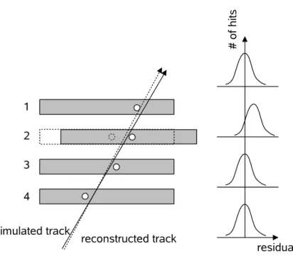
The distribution of the residuals belonging to one module is expected to be have a gaussian shape. For a detector module at nominal position the residual distribution is centred around zero, whereas for a misaligned module it will be shifted. This can be seen in figure 2.1. Module 2 is misaligned with respect to its nominal position; the residuals, which are calculated with respect to the nominal position, are biased, and therefore the distribution is shifted as well.

Different approaches of treating the minimisation of the residuals exist. The global χ² approach [39] tries to obtain the alignment parameters of all 5832 modules at once. This

13

(20)

14 Chapter 2. Kalman Style Alignment Approach (KASTRO)

residual

# of hits

reconstructed track simulated track

1 2 3 4

Figure 2.1: A simulated track crossing four detector modules. Module 2 is shifted with respect to its nominal position (dashed box). The effect on the track reconstruction (dashed line) and on the residual distribution (right) can be seen. [38]

involves an inversion of a 35k × 35k matrix and is a computational challenge. Another approach is the localχ² algorithm for the ATLAS Pixel and SCT detectors.

2.1 The local χ

²

approach

In this section the basic principles of the local χ² alignment algorithm for the SCT and the Pixel detectors is explained. A more detailed description can be found in [34, 38]. The local χ² alignment algorithm is a well proven method and has been used for alignment in other experiments before, e.g. for the BABAR Silicon Vertex Tracker (SVT) [40]. In ATLAS, it has been used with success for the silicon part of the Inner Detector. Monte Carlo studies of the whole Inner Detector setup as well as studies with real data on reduced setups in combined test beam and cosmic ray runs have been performed. As the name indicates, it is a local method, i.e. every detector module is treated separately.

The local approach works by minimising aχ² function given by:

χ²(~a, ~π₁, . . . , ~π_m) =

m

X

i ∈ tracks

~

r_i^T(~a, ~π_i)·V_i⁻¹·~r_i(~a, ~π_i). (2.1)

(21)

In this equation~r_i =~r_i(~a, ~π_i) contains the residuals of every module that was crossed by tracki. The residuals depend on the alignment parameters~aof the modules as well as on the track parameters~πi of the current track i. For a helical track model, the dimension of~π_i is 5. V_i denotes the covariance matrix of the residuals for tracki. The hits and thus the residuals are correlated due to the common track fit. That is why the rank of V_i is smaller than its dimension and it is per se not invertible. But since there are many hits present and the particular residual is calculated with respect to a track fit without taking the corresponding hit into account (reduced residual), this correlation can be neglected.

AssumingVi to be diagonal and neglecting module-to-module correlations, one can write down aχ²_k for every modulek:

χ²_k=

m

X

i∈ tracks

1

σ_ik² r²_ik(~a_k, ~πi). (2.2) σ_ik is the error of the residual r_ik of track i on module k. The vectors of alignment parameters~a_k have dimension 6, namely the six degrees of freedom of a module. The sum of theχ²_k returns theχ² from equation (2.1):

X

k∈ modules

χ²_k=χ². (2.3)

For a perfectly aligned module, theχ²_k is minimal with respect to~a_k: dχ²_k(~a)

d~a_k =~0, (2.4)

Equation (2.4) now describes the change in the χ²_k of one module with respect to its alignment parameters~a_kin all six degrees of freedom. For the sake of simplicity, the index kwill be omitted from now on.

Linearising the minimalχ² using a Taylor expansion yields:

dχ²(~a)

d~a ≈ dχ²(~a) d~a

_~_a=~_a

0

+ d²χ²(~a) d~a²

_~_a=~_a

0

∆~a. (2.5)

The expansion point~a0 contains the initial values of the six alignment parameters of the module and ∆~ais the difference between the current alignment parameters~aand~a₀. Now equation (2.5) is solved by applying equation (2.2) and setting all second order derivatives to 0:

dχ²(~a)

d~a =~0 = ^X

tracks

d d~a

1 σ²_ir²_i(~a)

! _~_a

=~a0

+ ^X

tracks

d² d~a²

1 σ²_ir²_i(~a)

! _~_a=~_a

0

∆~a=

= . . .= ^X

tracks

2 σ_i²

dr_i(~a) d~a0

!

ri(~a0) + ^X

tracks

2 σ²_i

dr_i(~a) d~a0

T!

∆~a (2.6)

(22)

16 Chapter 2. Kalman Style Alignment Approach (KASTRO) Here,^P_tracks means^P^m_i _∈ _tracksand _d~^d_a

0 is an abbreviation of _d~^d_a

~ a=~a0

. The solution for the alignment parameter correction ∆~ais:

∆~a=− ^X

tracks

1 σ_i²

dr_i(~a) d~a₀

T!−1

· ^X

tracks

1 σ_i²

dr_i(~a) d~a₀

r_i(~a₀)

!

. (2.7) The covariance matrix for the vector of alignment parameters is then given by [41]:

hC_~²_aⁱ= 2 d²χ² d~a²₀

!−1

≈ ^X

tracks

1 σ_i²

dr_i(~a) d~a0

T!−1

, (2.8)

and thus the error of the alignment parameters is:

σ_a_j =^qC²_a_jj. (2.9)

The following assumptions were made during the calculation of the alignment parameters

~afor one module:

• the covariance matrix of the residuals of a certain track is diagonal and the measurements on different detector surfaces are uncorrelated. The diagonal matrix is a result of the neglection of multiple Coulomb scattering. This can be justified by using only high momentum tracks, e.g. tracks with a momentum greater than 10 GeV.

Considering the use of reduced residuals (next item) the squared error of the residual σ² disentangles to a sum of the squared hit error and the squared track fit error σ²_hit+σ_track² .

• there is no contribution from the derivative of the residual with respect to the track parameters π_i:

dr_i(~a, ~π_i)

d~a = ∂r_i(~a, ~π_i)

∂~a +d~π_i d~a

dr_i(~a, ~π_i) d~πi

| {z }

≈0

(2.10)

This is ensured by using reduced track residuals where the hit on the module under consideration is removed from the track and a new track fit is performed before the residual is calculated.

• the dependence of the residual on the alignment parameters of other modules (k,l count modules) is set to 0:

dri k(~ak, ~πi) d~a_l

= 0! ∀ k6=l. (2.11)

This is only true if the error of the common track is small compared to the error of the given residual [34]:

σ_{T rack} σHit

2

<1. (2.12)

Recapitulating, a rather simple and easy to implement method how to calculate alignment parameters was presented. Because of the neglected correlations coming from equation (2.11), the local χ² approach intrinsically depends on iterations. The whole alignment procedure is repeated after applying the computed solutions of the alignment parameter to the detector geometry. The solution typically converges within O(10) iterations [38].

This process necessarily has a serious impact on the computing time.

(23)

2.2 Extension using KASTRO

The KAlman Style alignmenT appROach (KASTRO) extends the local χ² approach and tries to circumvent iterations. The alignment parameters are calculated recursively after each track is processed and the detector geometry is updated before the next event is processed. Whereas the local χ² algorithm collects all information and obtains the alignment parameters at the end, KASTRO uses the alignment information provided by the previously processed tracks immediately via the recursive calculation of the alignment parameters. In order to provide consistent results the geometry for the calculation of the residuals and the derivatives cannot be modified. This method has never been used before for alignment at a running experiment, so features of the approach have to be understood in the beginning. The use of a Kalman filter for alignment was first proposed by the CMS experiment [42].

2.2.1 Track fitting as example of a Kalman filter in high energy physics The idea and the name of the Kalman filter is attributed to Rudolph Emil Kalman who published his seminal paper ”A New Approach to Linear Filtering and Prediction Prob- lems” in 1960 [43].

The usage of the Kalman filter technique in high energy physics was then proposed by Rudolf Fr¨uhwirth in 1987 [44] and adopted by many experiments, e.g. DELPHI [45] at LEP and most recently, CMS [46] and ATLAS [47].

A Kalman filter is an efficient recursive filter which estimates the state of a dynamic system (state vector) by minimising the mean of the squared error [48]. The Kalman Filter can be used for linear and non-linear systems and has a wide variety of applications. The evolution of the state vector may proceed in time, as it does in radar tracking of a space- craft. This is actually the origin of the method. The state vector can also proceed in space as in the case of track fitting in a detector or along a dimensionless integer as in vertex fitting or alignment.

A Kalman filter is based on three operations:

• filtering is the estimation of the present state vector based upon all previous measurements.

• prediction is the estimation of the new state vector taking into account the latest measurement.

• smoothing is the estimation of the state vector for a previous measurement based upon all measurements.

A very illustrative example of a Kalman filter application is the track fitter of the ATLAS experiment named TrkKalmanFitter [49]. As mentioned above, the state vector (here:

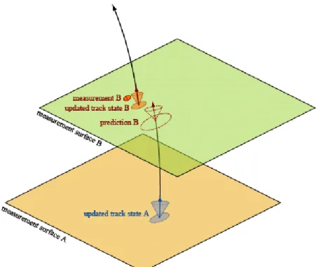
the five track parameters of a helical track model [50]) proceeds in space, namely from detector surface to detector surface.

Each Kalman filter step (cf. figure 2.2) involves two actions, the prediction and the filtering. Starting from a previous step or with an initial measurement, the track parameters and their errors are constrained on surface A. The errors of the track parameters are

(24)

18 Chapter 2. Kalman Style Alignment Approach (KASTRO)

Figure 2.2: A single filtering step in the TrkKalmanFitter. The different sizes of the ellipses and the cones indicate the change of the errors of the track parameters during a filtering step. [49]

represented by the ellipses and the cones in figure 2.2. In the prediction step, the track parameters and their errors are extrapolated to the next measurement surface B and form the prediction for the measurement on this surface. The filtering step combines the measurement on surface B with the prediction and results in an updated state on this surface.

These steps are then repeated for all measurements belonging to one track.

Since the Kalman filter steps can be executed both in the forward and in the reverse direction along the trajectory, the whole procedure is rerun starting from the endpoint.

This is the smoothing step. The forward predicted state is combined with the backward updated state on each surface to create the final state of the track parameters on all measurement surfaces. Here, the backward updated state is treated as the measurement on a certain surface and the corresponding forward predicted state is treated as the prediction on this surface. The combination procedure is the same as in the filtering step on surface B explained above.

Compared to a global track fitter likeIPatRec [51], the TrkKalmanFitterbecomes sensitive to track direction and momentum after just a few steps. The information gained from every Kalman filter step is used for the following step leading to a fast convergence on a stable result.

The TrkKalmanFitter will be referred to again in section 4 as it had to be modified for the implementation of KASTRO.

In the next section the mathematic derivation of the general Kalman filter formalism is presented.

(25)

2.2.2 Error weighted mean and Kalman gain matrix formalism

The state vector ~xk after k measurements is derived from a linear transformation Fk of the state vector~xk−1plus a random disturbanceω_k, the process noise. The measurements

~

m_k are linear functions of the state vector. This transformation is described by H_k and is corrupted by the measurement noise k. The covariance matrices Qk and G⁻¹_k corresponding toω_k and_k are assumed to be known. In the nonlinear case, the equations are approximated by their first-order Taylor expansions.

In the case of track fitting, explained above, ~xk holds the five track parameters and m~k

contains the measurements on detector surface k. F_k refers to the helical track model.

The function H_k maps the track parameters onto the measurements on detector surface k. The effect of matter on the trajectory is described by δk and k is the hit error.

~

xk =Fk~xk−1+ωk, < ωk>= 0, cov{ω_k}=Qk

~

m_k =H_k~x_k+_k, < _k>= 0, cov{_k}=G⁻¹_k (2.13)

In the following ~x_k|j denotes an estimate of the state vector based on the measurements

~

m₁, ..., ~m_j. Two cases must be distinguished:

• k > j: predicted estimate

• k=j: filtered estimate

Now it is supposed that a filtered estimate ~xk−1|k−1 based on the measurements

~

m1, ..., ~mk−1 exists along with its covariance matrix C_k−1|k−1 = C(~x_k−1|k−1).The prediction and the filtering step are needed to receive a new filtered estimate of the state vector~xk|ktaking into account the measurementsmk. The formulae for the prediction are [52]:

~xk|k−1 = Fk~xk−1|k−1

C_k|k−1 = F_kC_k−1|k−1F_k^T +Q_k (2.14)

The predicted state ~x_k|k−1 contains all the information from the measurements up to k−1. The first term of the covariance matrixC_k|k−1 is the linear error propagation of the previous covariance matrix while the second term refers to the process noise.

The filtered or updated state,~x_k|kis obtained as the error weighted mean of the prediction and the current measurement:

~x_k|k = C_k|kC_k|k−1⁻¹ ~x_k|k−1+H_k^TG_km~_k (2.15)

C_k|k =C_k|k−1⁻¹ +H_k^TG_kH_k⁻¹. (2.16)

(26)

20 Chapter 2. Kalman Style Alignment Approach (KASTRO) In the so called error weighted mean formalism, an inversion of a matrix of the size dim(~x)×dim(~x) is required to compute equation (2.16) and obtain the updated state.

In the gain matrix formalism, explained below, only an inversion of a matrix of the size dim(m)~ ×dim(m) is needed. It can be derived from the formulae (2.15) above.~

The Sherman-Morrison-Woodbury matrix identity is used for this [53]:

(A+U BV)⁻¹ =A⁻¹−A⁻¹UB⁻¹+V A⁻¹U⁻¹V A⁻¹ (2.17) where the dimensions of A are n×n, of U are n×l, of V are l×n , of B are l×l and l≤n. For the Kalman filter, nis the dimension of the state vector andl is the dimension of the measurement vector.

Applying equation (2.17) to the covariance matrix (2.16) and inserting the result in equation (2.15), the state vector is:

~

x_k|k=~x_k|k−1−C_k|k−1H_k^T G⁻¹_k +H_kC_k|k−1H_k^T⁻¹H_k~x_k|k−1+C_k|kH_k^TG_km~_k (2.18)

Reapplying equation (2.17) and using some matrix algebra, the equation of the state vector finally becomes:

~

xk|k=~xk|k−1+Kk

m~k−Hk~xk|k−1

(2.19)

with the Kalman gain matrix

K_k=C_k|k−1H_k^T G⁻¹_k +H_kC_k|k−1H_k^T⁻¹=C_k|kH_k^TG_k. (2.20) A more detailed derivation can be found in appendix A. In equation (2.20) one can see that the gain matrix formalism requires only the inversion of a matrix of the size dim(m)~ ×dim(m), namely the term in brackets. The updated covariance matrix~ C_k|k can also be computed without any inversion:

Ck|k= (I−KkHk)Ck|k−1 (2.21)

whereI is the unity matrix with the corresponding dimensions.

If the dimensions of the measurements are small compared to the dimension of the state vector and many measurements are present, a great deal of computing time can be saved using the gain matrix formalism.

The derivation of the formulae for the smoothing operation is omitted here. This step is not needed for alignment purposes as the system is static and no process noise is present.

The updated state of the alignment parameters is treated as the prediction for the next measurement and no extrapolation is needed as is the case for the TrkKalmanFitter (see section 2.2.1). Thus running the Kalman filter again in the reverse direction and combining the results will not lead to any improvement of the alignment parameters. The smoothing equations can be found in [52].

(27)

2.2.3 Kalman style extension of the local χ² approach

The solution of the alignment parameter correction ∆~a (equation (2.7)) can be directly transferred to the Kalman formalism. One module which acquirednhits is considered in the following. Then equation (2.7) becomes:

∆~a_n=−C_n·

n

X

i=1

1 σ_i²

dr_i(~a₀) d~a₀

r_i(~a₀)

!

(2.22) C_n is the covariance matrix of the alignment parameters aftern measurements:

Cn=

" _n X

i=1

1 σ²_i

∂r_i(~a₀)

∂~a0

∂r_i(~a₀)

∂~a0

T#−1

. (2.23)

By multiplying equation (2.22) with an identity matrix C_n−1⁻¹ ·Cn−1 and splitting up the nth term of the sum, equation (2.22) becomes:

∆~an=−C_n C_n−1⁻¹ Cn−1 n−1

X

i=1

1 σ_i²

dri(~a0) d~a0

ri(~a0) + 1 σ_n²

drn(~a0) d~a0

rn(~a0)

!

(2.24) One obtains a recursive formula applying the solution of equation (2.22) forn−1 Hits:

∆~a_n=−C_n

−C_n−1⁻¹ ∆~an−1+ 1 σ_n²

dr_n(~a₀) d~a₀

r_n(~a₀)

(2.25) Now equation (2.25) matches the Kalman filter in the error weighted mean formalism presented in equation (2.15). The state vector ~x_k in the Kalman formalism corresponds to ∆~an and the residual rn corresponds to the measurementm~_k, so the dimension of the measurement vector is 1 in this case. The matrixH_k^T corresponds to the vector ^dr_d~ⁿ_a^(~^a⁰⁾

0 , G_k is simply _σ¹2

n and the covariance matrices C_k|k and C_k|k−1⁻¹ of the Kalman filter are described here by−C_n and −C_n−1⁻¹ . The double index notation is no longer necessary as the filtered estimate of the alignment parameters is identical to the prediction for the next Kalman step.

An inversion of a 6×6 sized matrix is needed to obtain the covariance matrix of the alignment parameters in the error weighted mean formalism as can be seen in equation (2.23). If a covariance matrix C_n is present as a starting value for the Kalman filter, inversions of state vector sized matrices can be avoided for the following steps by using the gain matrix formalism and updating the covariance matrixC_n according to equation (2.21). Only inversions of matrices of the size of the measurement vector (here: one) have to be computed, as explained above.

Since the dimension of the state vector is six for the local alignment and is thus small, only a small amount of computing time can be saved by using the gain matrix formalism.

It was therefore decided to implement the more generic error weighted mean formalism.

The starting value of the state vector plays a crucial role for the Kalman filter. It was chosen to apply the solution of the local χ² approach as initial prediction as soon as the inversion of the matrix in equation (2.7) ceases to fail. Depending on the quality of the hits on the module, the inversion is usually successful after three to eight hits have been acquired.

(28)

Chapter 3

Prototype simulation with ROOT

The first major part of this diploma thesis was the combination of two standalone imple- mentations of the localχ² algorithm for the SCT and the Pixel detectors. Subsequently, the KASTRO formalism was applied to the combined prototype programme and tested.

3.1 ROOT software

ROOT is a C++-based programme that has been developed mainly for data analyses in high energy physics. Thanks to the approach of loosely coupled object-oriented frameworks it has been extended to cover other domains like event generation, detector simulation and event reconstruction as well [54].

ROOT was chosen to be the environment for the two prototype programmes studying the feasibility and the performance of the localχ² alignment algorithm for the Pixel and the SCT detectors. Compared to the complicated ATLAS software framework (Athena), ROOT provides a more flexible and independent setup. In a first step, the two standalone programmes were combined into a single one such that one can easily switch between the particular module types.

3.2 Geometry setup and tracking

Since a local approach aligns each detector module separately, only a single module of each kind needs to be studied within the prototype programme. The geometry setup of the different module types was adopted from the existing prototype programmes. The two modules considered are barrel modules sitting atη≈0.

The design of a particular module follows closely the descriptions given in subsections 1.4.1 and 1.4.2. The local and global coordinate frames for the two module types are the same as the ATLAS coordinate frames described in section 1.5. A ROOT GeoModel graphic of the modules can be seen in figure 3.1.

To evaluate the basic properties of the approach, a simple track model is used, i.e perfect straight line tracks coming from a common vertex that has the global coordinates (0, 0, 0).

22

(29)

Figure 3.1: Drawing of the modules. A simple ROOT GeoModel graphic of the SCT (left) and the Pixel (right) module is shown here. One can see the two rotated detector surfaces of the SCT. The simulated readout strips and pixels are not visible here.

The modules are placed in the global coordinate system at (1.72 cm, 4.74 cm, 0) for the Pixel module or (20 cm, 44 cm, 0) for the SCT module and illuminated uniformly.

The hits on the detector surfaces are then produced by calculating the associated readout channel closest to the impact point of the track with the detector surface. Cluster effects, which occur when more than one readout channel is associated with a particular hit, are not taken into account in the prototype programme. Due to the simple tracking model, the track comes with no error.

3.3 Implementation of KASTRO

The input quantities of both the localχ² approach and of KASTRO are residuals, derivatives of the residuals with respect to the alignment parameter and errors of the residuals as described in equations (2.25) and (2.7).

3.3.1 Residuals

Residual definitions frequently used for alignment purposes are in-plane residualsrin−plane

and Distance Of Closest Approach (DOCA) residualsrDOCA.

In Athena, it was chosen to implement DOCA residuals. They are simple to calculate and the residual derivatives using DOCA residuals are also easy to compute. The computation of the in-plane residuals is often incorrect, especially in the endcap regions of the SCT detector due to the wedge-shaped form of the modules and the varying strip pitch.

In-plane residuals

The in-plane residuals are defined as the smallest distance on the detector surface between the impact point of the track and its associated hit. For the Pixel module, two residuals belonging to one hit are calculated; one with respect to a virtual readout strip crossing

(30)

24 Chapter 3. Prototype simulation with ROOT

DOCA residual

particle track impact point

in-plane residual readout strip

x y

virtual readout-strips

in-plane residual pixelcenter

DOCA residual

particle track impact point

y x

Figure 3.2: Definition of the residuals. The definition of in-plane (blue) and DOCA (red) residuals are indicated for the SCT module (top) and the Pixel module(bottom).

the pixel centre in the x direction and one with respect to a virtual readout strip crossing the pixel centre in the y direction. In the SCT case, two residuals are computed as well;

one with respect to the readout strip for each detector surface:

r_a r_b

!

in−plane

= aimpact point−a_readout bimpact point−b_readout

!

(3.1) where (a, b) = (x, y) (Pixel) or (a, b) = (x_rφ, x_stereo) (SCT).

DOCA-residuals

The DOCA residuals are calculated as the smallest distance between two straight lines.

One line always represents the straight line track and the other line is either the readout strip of a SCT wafer or a virtual readout strip going trough the pixel centre as mentioned above. The different definitions of the residuals are shown in figure 3.2. Assuming two straight lines with the parametrisations

~x=





 a₁ a2

a₃





+λ





 b₁ b2

b₃





 (3.2)

(31)

for the straight line track and

~x⁰ =





 c1

c₂ c3





+κ





 d1

d₂ d3





 (3.3)

for the readout strip, the signed shortest distance can be computed via determinants [55]:

r_DOCA=

a₁−c₁ a₂−c₂ a₃−c₃

b₁ b₂ b₃

d1 d2 d3

v

u u t

b1 b2

d1 d2

2

+

b2 b3

d2 d3

2

+

b3 b1

d3 d1

2 (3.4)

The in-plane residual can be calculated analytically from the DOCA residualr_DOCA. A drawing for the residuals with respect to the y axis is shown in figure 3.3. The functional relation of the residuals is given by:

r_DOCA = sin

cosδ rin−plane≡f(~a) rin−plane (3.5) where is the incident angle of the track andδ is the angle in the x-y plane as sketched in figure 3.3.

y x z

. .

.

^^r^DOCA

r

r_in−_plane

t

 n





track

readout strip

Figure 3.3: Sketch of r_DOCA and rin−plane and the related quantities. Here the x-residuals are shown.

The DOCA residualr_DOCAand the linearised track vector~tare needed for the calculation ofrin−plane. Since the DOCA residual is calculated as the smallest distance between two straight lines the vector~r_DOCAis perpendicular to the readout strip running in y direction