RESEARCH ARTICLE
10.1002/2016GC006662
Linking basin-scale and pore-scale gas hydrate distribution patterns in diffusion-dominated marine hydrate systems
Michael Nole1 , Hugh Daigle1 , Ann E. Cook2 , Jess I. T. Hillman2,3, and Alberto Malinverno4
1Department of Petroleum and Geosystems Engineering, University of Texas at Austin, Austin, Texas, USA,2School of Earth Sciences, Ohio State University, Columbus, Ohio, USA,3GEOMAR Helmholtz Centre for Ocean Research, Kiel, Germany,4Lamont Doherty Earth Observatory of Columbia University, Palisades, New York, USA
Abstract
The goal of this study is to computationally determine the potential distribution patterns of diffusion-driven methane hydrate accumulations in coarse-grained marine sediments. Diffusion of dissolved methane in marine gas hydrate systems has been proposed as a potential transport mechanism through which large concentrations of hydrate can preferentially accumulate in coarse-grained sediments over geologic time. Using one-dimensional compositional reservoir simulations, we examine hydrate distribution patterns at the scale of individual sand layers (1–20 m thick) that are deposited between microbially active fine-grained material buried through the gas hydrate stability zone (GHSZ). We then extrapolate to two-dimensional and basin-scale three-dimensional simulations, where we model dipping sands and multilayered systems. We find that properties of a sand layer including pore size distribution, layer thickness, dip, and proximity to other layers in multilayered systems all exert control on diffusive methane fluxes toward and within a sand, which in turn impact the distribution of hydrate throughout a sand unit. In all of these simulations, we incorporate data on physical properties and sand layer geometries from the Terrebonne Basin gas hydrate system in the Gulf of Mexico. We demonstrate that diffusion can generate high hydrate saturations (upward of 90%) at the edges of thin sands at shallow depths within the GHSZ, but that it is ineffective at producing high hydrate saturations throughout thick (greater than 10 m) sands buried deep within the GHSZ. Furthermore, we find that hydrate in fine-grained material can preserve high hydrate saturations in nearby thin sands with burial.Plain Language Summary
This study combines one-, two-, and three-dimensional simulations to explore one potential process by which methane dissolved in water beneath the seafloor can be converted into solid methane hydrate. This work specifically examines one end-member methane transportmechanism, diffusion, and its potential to help grow methane hydrate in the pore space of marine
sediments. The simulations presented here span hundreds of thousands of years to capture the evolution of a diffusion-dominated gas hydrate system over geologic time.
1. Introduction
Gas hydrates are ice-like compounds composed of low molecular weight gases trapped in water lattices that are stable at high pressure and low temperature [Sloan and Koh, 2007]. Naturally occurring hydrates typically contain methane as the guest molecule, so accumulations of hydrate worldwide constitute uncon- ventional reservoirs of natural gas. Natural methane hydrates can form within the sediments of any subsur- face environment globally where the appropriate thermodynamic conditions for stability are met and enough dissolved gas is available to come out of solution and precipitate as a solid [Kvenvolden, 1998;Buf- fett, 2000]. These conditions most commonly exist along marine continental margin environments as well as under arctic permafrost [Paull and Dillon, 2001]. Methane hydrate deposits are increasingly of interest worldwide for their resource potential [Collett, 2002] as well as their ability to impact global climate change [Dickens et al., 1995] and submarine slope stability [Mienert et al., 2005].
In the Gulf of Mexico, salt-withdrawal basins of the outer continental shelf have been the subject of much attention in recent years due to their abundance of naturally occurring methane hydrate deposits.
Methane hydrate accumulations in the area have historically been investigated for their potential as a drilling hazard [Milkov et al., 2000]; more recently, they have come to be viewed as a potential energy
Key Points:
We show potential distribution patterns of methane hydrate that can preferentially accumulate in coarse- grained sands via diffusion
One-dimensional simulations demonstrate the impact of pore size distributions and sand layer thickness on gas hydrate distributions within sand layers
In 2-D and 3-D, concentration gradients in multiple dimensions and competition between sand layers can limit methane transport
Correspondence to:
M. Nole,
michael.nole@utexas.edu
Citation:
Nole, M., H. Daigle, A. E. Cook, J. I. T.
Hillman, and A. Malinverno (2017), Linking basin-scale and pore-scale gas hydrate distribution patterns in diffusion-dominated marine hydrate systems,Geochem. Geophys. Geosyst., 18, 653–675, doi:10.1002/
2016GC006662.
Received 29 SEP 2016 Accepted 2 FEB 2017
Accepted article online 7 FEB 2017 Published online 23 FEB 2017
VC2017. American Geophysical Union.
All Rights Reserved.
Geochemistry, Geophysics, Geosystems
PUBLICATIONS
resource [Boswell et al., 2012;Frye, 2008]. A location in Walker Ridge Block 313 (WR313) in the Terre- bonne Basin is an interesting site with a variety of hydrate reservoirs and hydrate morphology.
Logging-while-drilling (LWD) data collected at the Terrebonne Basin by the Chevron-DOE Joint Industry Project (JIP) indicated high hydrate saturation occupying the pore space of both thick sand reservoirs (10–25 m scale) and thin isolated sand layers (3 m or less). Fracture-hosted hydrate in fine-grained sediments was also identified, with one such unit over 100 m thick [Frye et al., 2012]. In addition to the LWD data from two wells, 2-D and 3-D seismic data has been acquired in the Terrebonne Basin [Frye et al., 2012;Haines et al., 2014].
Interpretations of well log and seismic data in this region provide different hypotheses for the dominant methane migrations mechanisms at play to produce observed saturations of methane hydrate. Advective, updip methane flux through sandy strata from a deep methane source has been proposed as a potential transport mechanism for thick, deep hydrate deposits (near the BHSZ) in the region, as regional seismic interpretation indicates the presence of a free gas phase beneath the BHSZ [Boswell et al., 2012;Frye et al., 2012]. Since hydrate forms in pore space and reduces sediment permeability, high hydrate saturations in thin sands have also been implicated in overpressure generation and fracturing in advective systems; one- dimensional (1-D) models have been developed to explain such occurrences and the time scales over which they can develop [Daigle and Dugan, 2010;Daigle and Dugan, 2011]. Furthermore, flow focusing as an advective fluid transport mechanism in overpressured marine systems can enhance methane transport in the presence of clay-sand effective methane solubility contrasts [Nole et al., 2016]. These mechanisms can charge thick or thin sands alike, while high hydrate saturations generated by a diffusive transport mecha- nism tend to be found mainly in thin sands.
Well log data and 1-D modeling of sands at WR313 have been used to suggest a dominantly diffusive migration mechanism in shallow, thin sands from microbially produced methane in clayey strata adjacent to a 2.5 m thick sand layer [Cook and Malinverno, 2013]. High hydrate saturations in the pores of thin, sandy layers [Frye et al., 2012] are also observed in some locations to occur between fracture-hosted hydrates in bounding clays [Cook et al., 2008]. The presence of hydrate-free zones separating hydrate in clays from hydrate in sands has been suggested as evidence that diffusion along clay-sand spatial solubility disconti- nuities can act as a dominant transport mechanism to supply methane to thin, shallow sands [Malinverno, 2010;Cook and Malinverno, 2013;Malinverno and Goldberg, 2015].
At the reservoir scale, gas hydrate systems modeling solves coupled systems of mass and energy conserva- tion equations to explain observations unique to different hydrate-bearing environments. One-dimensional modeling has been performed to describe gas hydrate accumulations in marine sediments under varying fluid flux conditions, methanogenesis rates, and sedimentation rates [Davie and Buffett, 2001, 2003;
Bhatnagar et al., 2007;Garg et al., 2008]. This methodology has been expanded into 2-D, where effects of permeability anisotropy, gas buildup beneath the base of the hydrate stability zone (BHSZ), and sediment fracturing on methane hydrate accumulations in porous media have been compared to 1-D simulation results and well log interpretations [Chatterjee et al., 2014]. These studies have provided useful benchmarks for better understanding dynamic hydrate systems. We build upon their methods by incorporating pore size distribution effects on methane solubility, employing a Lagrangian reference frame in 1-D and 2-D with a rhombic grid system for 2-D simulations, and performing 3-D simulations with time-varying grid proper- ties with a modeled basin stratigraphy informed by interpreted seismic data.
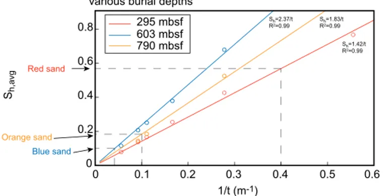
The goal of this study is to computationally determine potential gas hydrate distribution patterns in coarse- grained sand layers where diffusion is the dominant methane transport mechanism. We simulate diffusion- dominated gas hydrate systems in one, two, and three dimensions similar to that of the Terrebonne Basin in the Gulf of Mexico. In our models, we consider a range of sand thicknesses varying from 3 m (similar to the thin sand described byCook and Malinverno[2013]), which we refer to as the Red Sand, to 10.5 and 25 m, which we call the Orange and Blue Sands respectively and are similar to those encountered in the Terrebonne Basin [Frye et al., 2012]. We employ 1-D and 2-D simulations in a moving reference frame to understand local hydrate accu- mulations within and immediately surrounding a thin sand layer. We then expand to a 3-D reservoir model to assess hydrate distribution patterns on a regional scale between multiple dipping sand bodies. We show that at a local scale, capillary inhibition with hydrate growth can progress from the outer boundary toward the center of a sand body [Rempel, 2011], causing a smoothing effect on hydrate saturation distributions throughout the
sand. On a regional scale, we show that the geometry of sand layers as well as the spatial relationship between multiple dipping sands can dramatically influence gas hydrate distribution patterns.
2. Methods
Simulations performed in this study build upon the methane hydrate reservoir simulator developed bySun and Mohanty[2006]. The simulator uses a fully implicit, finite volume difference scheme with primary vari- able switching to solve a coupled system of mass balance equations for water and methane along with a system energy balance. The simulator is stable on large length scales and over geologic timespans. Hydrate formation and dissolution are tracked by assuming local equilibrium corresponding to the thermodynamic state of each grid block. If a grid block contains dissolved methane in concentrations exceeding the aqueous-phase solubility at a given pressure and temperature, excess methane partitions into the hydrate and/or gas phase. The model domains employed in this work are situated entirely within the gas hydrate stability zone (GHSZ), so methane in excess of aqueous solubility only forms hydrate.
We made several modifications to the simulation methodology for the work presented here. The pore water in shallow marine sediments is saline, and the addition of a salt component alters the equilibrium solubility conditions of methane in pore water. Hydrate forms in confined sediment pore space, which alters the Gibbs free energy of the pore system in comparison to a bulk system and results in a phenomenon known as the Gibbs-Thomson effect [Clennell et al., 1999]. An increase in effective methane solubility due to the Gibbs-Thomson effect is significant in the small pores of fine-grained, clay-rich sediments. Pore space in sediments is characterized by a distribution of pore sizes, so the increase in solubility due to the Gibbs- Thomson effect should become more significant as gas hydrate saturation increases, filling progressively smaller pores [Liu and Flemings, 2011]. In marine environments, methanogens beneath the seafloor work to convert buried organic matter to methane, constituting a major source of methane in hydrate-bearing sedi- ments in addition to methane produced by thermogenic processes. Organic matter is mostly preserved in fine-grained sediments [Hedges and Keil, 1995], and methanogenesis is active in clay-rich units [Claypool and Kaplan, 1974]. Furthermore, the simulated system is not static; sedimentation consistently pushes sedi- ment layers downward relative to the seafloor, increasing temperature and pressure, which in turn affect hydrate formation and dissolution. Throughout this process, compaction of pore space reduces porosity, resulting in upward fluid motion with respect to solid sediment grains [Berner, 1980].
2.1. Salt Mass Balance in Pore Water
Our methane hydrate reservoir simulator makes use of an empirical three-phase equilibrium pressure- temperature (P-T) correlation for Structure I methane hydrate in a bulk system of pure water [Moridis, 2003].
In marine hydrate-bearing environments, the P-T curve is affected by the presence of dissolved salt in pore fluid, which inhibits hydrate formation [Koh et al., 2002].
For the purposes of marine sediment simulations, the P-T curve can be translated by a temperature incre- mentDThydif salt is present in the pore water, given by the following equation [Sloan and Koh, 2007]:
DThyd
TwðTw2DThydÞ50:6652 DTfus
TfðTf2DTfusÞ; (1)
whereTwis the freezing temperature of hydrate in a salt-free system,DTfusis the hydrate freezing tempera- ture depression at atmospheric pressure for a given salt mass fraction, andTf is the freezing temperature of water. The hydrate freezing temperature depression at atmospheric conditions is calculated from data tabu- lation as follows [Haynes and Lide, 2010]:
DTfus5wsA164:49wAs149:462
; (2)
wherewsAis the mass fraction of salt in the aqueous phase, in kg salt/kg fluid. The P-T diagram is thus trans- lated as follows:
T5T01DThyd; (3)
whereT0is the in situ pore water temperature, andT is the temperature in pure water whose equilibrium pressure would correspond to the equilibrium pressure of a saline system atT0. In the presence of dissolved
salt, hydrate precipitates at a lower temperature for a given pressure (or at a higher P for a given T) com- pared to pure water.
Additionally, when methane hydrate forms in pore space, pure water and methane are the only two constit- uents of the hydrate phase. Salt in the pore water is therefore excluded from the hydrate phase, and because water is consumed upon formation of hydrate, the pore water salt concentration increases. This leads to a situation whereby hydrate formation locally increases pore water salt concentration, which in turn increases methane solubility in the pore water, inhibiting the formation of methane hydrate until the excess salt diffuses out or less saline water flows in.
2.2. The Gibbs-Thomson Effect
Methane hydrate formation occurs when the concentration of methane dissolved in pore water exceeds its solu- bility at a specified pressure, temperature, and pore water salinity. Additionally, decreasing the size of a pore increases the surface area to volume ratio of the pore space, and hydrate crystals that nucleate in these pores must have correspondingly large surface area to volume ratios. In fine-grained sediments, the increase in curva- ture of the interface between a nucleating mass of hydrate and surrounding pore water is significant enough that the contribution of interfacial energy to the total Gibbs free energy of the pore water-methane system can- not be neglected. This in turn leads to an increase in the solubility of methane in the pore space, inhibiting hydrate growth [Clennell et al., 1999].
An increase in methane solubility with decreasing pore radius corresponds to a decrease in the equilibrium triple point temperature of methane in the pore space, known as the Gibbs-Thomson effect. Thus, methane hydrate requires lower temperatures for nucleation in smaller pores than in larger pores, all else being equal. This phenomenon is implemented in the simulator as a translation of the phase diagram dependent on the effective pore radius of the grid block of interest. The change in methane hydrate freezing tempera- ture is calculated as follows [Anderson et al., 2009]:
DTm522Tmbrhlcosð Þh
Hfqhre ; (4)
whereTmbis the freezing temperature of methane hydrate in bulk water,rhlis the solid-liquid interfacial energy between hydrate and water,his the hydrate wetting angle to the pore surface,Hfis the hydrate bulk enthalpy of fusion,qhis the density of methane hydrate, andreis the effective pore radius describing the change in freezing temperature in a pore of radiusre.
For a given in situ temperatureT0within the pore space, the temperature is therefore adjusted when calculating the hydrate freezing pressure as follows before being used to calculate the corresponding three-phase equilibri- um pressure:
T5T0 112rhlcosð Þh Hfqhre
: (5)
2.3. Steady State Methanogenesis
In the shallow subsurface of marine methane hydrate-bearing environments beneath the sulfate reduction zone, microbes known as methanogens convert organic material that has been deposited on the seafloor into methane [Claypool and Kaplan, 1974]. Methanogens typically act in organic-rich, clayey sediments and are inactive in sandy units [Waseda, 1998;Pohlman et al., 2009]. Because the average pore size in clays is smaller than that in sandy layers, the solubility of methane in fine-grained layers is higher than the solubility of methane in the sands. Also, as the organic matter in the clayey layers is consumed by methanogens, less organic matter remains and therefore less methane is produced as burial proceeds.
A dynamic system therefore typically exists with respect to methanogenesis in marine gas hydrate systems.
At steady state, the microbial methane production rate can be expressed as a decreasing function of depth as organic matter is consumed. Methanogenesis only takes place in the presence of organic matter, which is often associated with fine-grained sediments, and since these sediments can hold more aqueous meth- ane in solution than the coarse-grained sand layers due to their small pore sizes, aqueous methane concen- tration gradients typically exist between clayey and sandy layers [Malinverno, 2010]. This drives a diffusive flux from fine-grained clays to coarse-grained sands, promoting hydrate growth in the coarse-grained layers
due to short diffusive migration of methane, or diffusive methane transport between adjacent layers within the GHSZ.
Steady state methane generation due to microbial methanogenesis is implemented following the formula- tion ofMalinverno[2010] as follows:
q zð Þ5kakaSMTe2xkðz2zSMTÞ; (6) whereq(z) is a 1-D depth-varying source of methane into the pore space,kais a conversion factor from metabolizable organic carbon mass fraction to dissolved methane concentration,kis the reaction rate of microbial methanogenesis, aSMT is the mass fraction of metabolizable organic carbon at the sulfate- methane transition (SMT),xis the sedimentation rate, andzSMTis the depth below seafloor of the SMT. To justify a steady state methanogenesis assumption, the domain simply assumes that methanogens are already present in clayey strata throughout the sediment column as an initial condition. This depth-varying methane source term is imposed only upon grid blocks specified as clay and not sand.
2.4. Sedimentation
Over geologic time, sedimentation works not only to consolidate sediments, as has commonly been investi- gated with marine hydrate simulations, but it also brings in sediments with heterogeneous physical proper- ties as sediment sources and depositional environments change. Because lithology can exert an important control on permeability, porosity, and pore size distribution in the subsurface, our simulations incorporate lithologic heterogeneity by formulating all relevant grid properties as functions of time and space.
For the environments simulated here, a binary system of sand and clay strata was considered, although in reality geologic systems are certainly more complicated. To identify the sand units in the stratigraphic col- umn in the Terrebonne Basin, logging-while drilling well log data was analyzed from two JIP Leg 2 wells [Collett et al., 2012]. Then, to extend the stratigraphic interpretation over the basin, the well logs were tied to 3-D seismic data by developing synthetic seismograms for each well. Information describing the Red, Blue, Orange, and Green sands [Frye et al., 2012] was then fed into the 3-D simulator as latitude, longitude, and depth coordinates corresponding to the mapped top and bottom surfaces of the sand layers. All grid blocks outside of the sand horizons are considered to be clay. Different lithologies can easily be incorporat- ed using this method by simply making the grid block designations dependent on the specific imported horizon.
Once the sand layers are loaded into the grid, the 3-D simulations use a sedimentation velocity and simula- tion end time to determine the depth at present time that would correspond to the seafloor depth at the beginning of the simulation. The position and orientation of each sand layer as a function of time are inter- polated between the initial sand layer geometries at deposition and their current observed geometries. In the simulations presented in this study, sand layers are deposited originally as horizontal beds whose dip and depth increase with burial. Although a constant sedimentation velocity characterizes each grid block, the sedimentation velocity can vary laterally, resulting in an evolving dip of the sand layers. The solid hydrate phase is carried downward with sedimentation. While this is a simplification of depositional history and does not capture more dynamic geologic processes pertaining to uplift and deformation, it is sufficient for our purposes to capture first-order effects of sand layer burial and rotation on hydrate accumulation patterns.
2.5. Grid Formulations, Boundary Conditions, and Initial Conditions
One- and two-dimensional simulations were performed on a small scale to assess the impact of methane diffusion on gas hydrate distributions within and immediately surrounding a thin sand layer as it is buried through the GHSZ. In these simulations, we adopt a Lagrangian reference frame: boundary conditions change through time in the simulation to reflect increasing pressure and temperature with burial. The sys- tem pressure is adjusted by adding hydrostatic pressure throughout the domain at each time step accord- ing to the change in burial depth, and the temperature is correspondingly adjusted by increasing temperature according to the geothermal gradient. The methane concentrations at the boundaries of the domain, away from the sand layer, are set to the steady state solution without a sand layer present (the steady state solution is time-invariant and does not need to be solved at each time step). Methane concen- trations change as a result of changing methanogenesis rates, which are also adjusted throughout the
domain at each time step. The time step is variable and changes according to rate of solution convergence, with a minimum time step of approximately 200 days. Three-dimensional simulations were performed in an Eulerian reference frame with static boundary conditions; as coarse-grained sand layers are buried through the domain, new fine-grained material is deposited on top.
The 1-D simulation control volume is depicted in Figure 1. In these simulations, a compaction-driven flux boundary condition varies with time at the bottom of the domain. Compaction moves fluid upward relative to the sediment grains and diminishes as the change in porosity of the system with burial approaches zero.
This stands in contrast to a fixed reference frame (as in the 3-D simulations performed here), in which compaction-driven fluid flow is downward when the reference frame is fixed at the seafloor [e.g.,Bhatnagar et al., 2007;Frederick and Buffett, 2011]. The top of the domain is kept at a constant pressure corresponding to hydrostatic pressure at the depth of the boundary. While this pressure may not be exactly hydrostatic (if fluid is moving upward above the domain), the magnitude of any overpressure in this control volume due to compaction flux has a negligible impact on methane solubility throughout the domain. Boundary tem- peratures are fixed along a geothermal gradient. The simulation boundaries are placed sufficiently far from the sand such that hydrate growth in the sand is separated from hydrate in clays by hydrate-free zones. Ini- tially, methane is absent from the system at the SMT, and the methane concentrations on the top and bot- tom boundaries are set equal to the methane concentrations in their respective adjacent grid blocks with the addition of dissolved methane due to methanogenesis on the boundaries. All grid blocks in 1-D are 0.6 m thick. The thickness of the entire sand layer varies from 1.8 to 18 m with 25.5 m of clay both above and below the sand layer, for a total domain length of between 52.8 and 69 m.
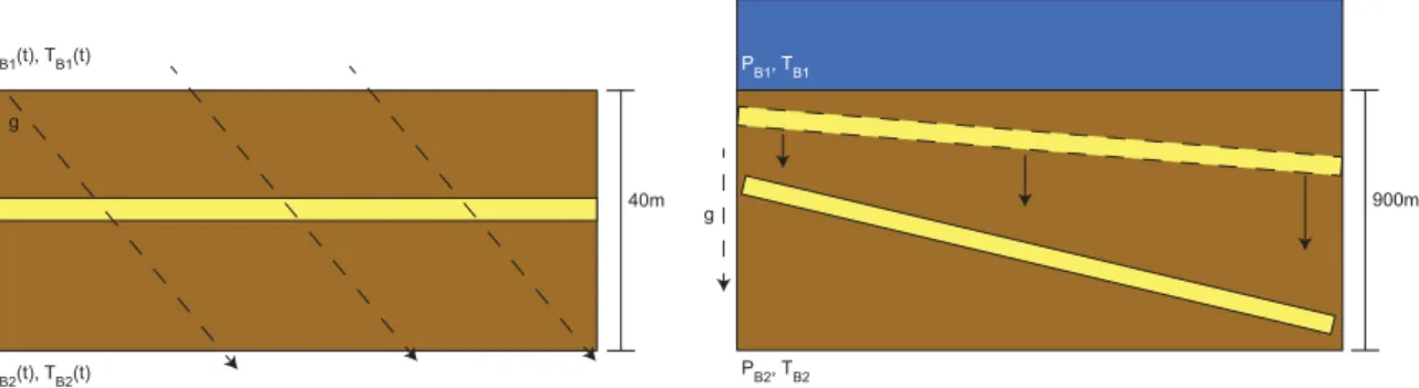
In 2-D, the simulation domain is discretized into an array of right rhombic prisms; the gravity vector is rotat- ed to simulate a dipping sand(Figure 2a). This is important because in a rectangular grid system oriented orthogonal to gravity, the edge of a dipping sand must be described by a discrete step function, across which diffusion can act laterally and vertically. When the scale of grid discretization is on a similar order of magnitude to the thickness of the sand itself, a jagged sand edge could yield unwanted methane diffusion
Methane concentration
Depth below seafloor
Fine-grained sediment Coarse-grained sediment Simulation Control Volume
Free-space methane solubility
Higher effective solubility in small pores
Depth below seafloor
Seafloor
t
1PB1,TB1,CmB1
PB2,TB2,CmB2 ZB2
ZB1
t
2 PB1,TB1,CmB1PB2,TB2,CmB2 ZB2
ZB1
ZB1 = vsed*t1
ZB2 = ZB1 + hCV
hCV
ZB1 = vsed*t2
ZB2 = ZB1 + hCV
hCV
Figure 1.(left) A fully developed methane concentration profile in a repeating sequence of alternating fine- and coarse-grained sediments with the free space methane solubility (dashed green line) and clay layer methane solubility (dashed magenta line) superimposed. (right) The control volume in 1-D centers around a sand layer that is buried over time. Bound- ary conditions change with time.
parallel to the sand surface. Boundary conditions are formulated in the same way as described for 1-D simu- lations. Also as in 1-D, the system is initially devoid of methane, so the hydrate formation and dissolution patterns reflect the maximum amount of hydrate dissolution possible for a given set of methanogenesis parameters. On the top and bottom boundaries, methane concentrations are formulated as functions of time in the same way as in 1-D simulations: at each time step, the methane concentration on each bound- ary is set to the methane concentration in the grid block adjacent to the boundary at the previous time step plus the addition of methane due to methanogenesis on the boundary. On the sides of the domain, no flux boundary conditions are prescribed for methane concentrations. The simulated sand layer is discretized as one 3.6 m grid block. The downdip length of the sand layer in these simulations is set at 100 m, discre- tized into 20 grid blocks. Though compaction-driven flow can focus in the high-permeability sand layer in the 2-D simulations, discussion of flow focusing is beyond the scope of this work.
In 3-D, a static system in an Eulerian reference frame buries sand layers through a fixed domain (Figure 2b).
The top boundary is set at seafloor hydrostatic pressure, the bottom boundary condition is that of constant advective compaction flux, and constant temperature boundary conditions on the top and bottom of the domain are defined by the geothermal gradient. As initial conditions, methane concentrations and methane hydrate saturations throughout the domain are set to zero; therefore, the results of these simulations yield maximum dissolution rates for a given set of environmental parameters. The 3-D grid is comprised of 11,250 grid blocks (50 in the downward z direction and 15 in each lateral dimension), discretizing a basin system that spans 13.3 km by 9.8 km laterally and 915 m in the depth dimension. This resolution yields a sand grid block vertical thickness of 18.3 m, which is about 5 times the thickness of the individual sand unit modeled in 2-D.
One- and two-dimensional simulations are limited in that they cannot describe regional-scale gas hydrate distribution patterns; 1-D simulations illustrate hydrate distributions within a sand layer itself, while 2-D sim- ulations demonstrate how methane solubility gradients in multiple directions affect average hydrate satura- tions in and around a thin sand layer. The benefit of 1-D and 2-D simulations is that they provide results at a resolution not possible in 3-D simulations due to computational limitations. Three-dimensional simulations are therefore not able to resolve hydrate-free zones immediately surrounding sand layers; nor can they depict gas hydrate distributions within individual sands. They do, however, illustrate regional gas hydrate distribution trends across multiple dipping, nonplanar sands. To ensure consistency of the numerical meth- ods between 1-D, 2-D, and 3-D simulations, all simulations are run using a finite volume methodology. All simulations are run in 3-D; the second and third dimension are rendered trivial in 1-D simulations, and the third dimension is rendered trivial in 2-D simulations.
2.6. Incorporating Observations From Well Logs, Laboratory Measurements, and Seismic Data 2.6.1. Observations at the Terrebonne Basin
In the Terrebonne Basin, the JIP Leg 2 drilled two wells, hole WR313-G and hole WR313-H, targeting two res- ervoir sand units near the base of the gas hydrate stability zone: the Blue sand and the Orange sand [Boswell et al., 2012;Frye et al., 2012]. Logging-while-drilling measurements revealed that the Blue sand unit contains sandy layers interbedded with clays for a total hydrate-filled sand of25 m, whereas the deeper
b) Eulerian reference frame: static boundary conditions
g g
40m PB1(t), T
B1(t)
PB2(t), TB2(t)
900m PB1, TB1
PB2, TB2 a) Lagrangian reference frame: time-varying boundary
conditions, non-orthogonal angle of gravity.
Figure 2.(a) A moving (Lagrangian) reference frame is used for 1-D and 2-D simulations of hydrate distributions within and around single sand layers. Dashed lines represent the gravity vector, which rotates to simulate the dip of the sand in 2-D. (b) A static (Eulerian) reference frame is implemented in this study for 3-D basin-scale simulations.
20 60 100
Depth (mbsf)
820
825
830
835
840
845
850
855
860
865
870
875
Gamma Ray (API)
0.2 0.4
Density Porosity (fraction of bulk sediment)
10-1 100 101 102 Resistivity
(ohm*m ) Ring Ro
0 0.5 1
Hydrate Saturation (fraction of pore space)
n=2.0 n=2.5 n=3.0
20 60 100
804
806
808
810
812
814
816
818
820
0.1 0.2 0.3 0.4 10-1 100 101 102 0 0.5 1
Depth (mbsf)
a. b. c. d.
Blue Sand in WR313-G
Orange Sand in WR313-H
Gamma Ray (API)
Density Porosity (fraction of bulk sediment)
Resistivity (ohm*m)
Hydrate Saturation (fraction of pore space)
e. f. g. h. n=2.0
n=2.5 n=3.0 Ring
Ro
Figure 3.Measured and calculated logs from (a–d) Hole WR313-G Blue sand unit and (e–h) Hole WR313-H Orange sand unit in meters below seafloor (mbsf). Interpreted hydrate-bearing sands are highlighted in green. Figures 3a and 3e show the measured gamma ray log, which indicates sandier layers to the left (lower API) and clay-rich layers to the right (higher API). Figures 3b and 3f show the density porosity, which is corrected for the hydrate saturation. The measured ring resistivity is shown in Figures 3c and 3g along with R0, the resistivity of the formation in the absence of hydrate. The calculated hydrate saturation is presented in Figures 3d and 3h.
Orange sand was comprised of two main lobes for a total of 10.5 m of hydrate-filled sand (Figure 3a). Thick- nesses reported here are larger than byFrye et al. [2012] andBoswell et al. [2012], as they only considered high saturation (Sh>0.5) gas hydrate. In our models, we are interested not just in high saturations of hydrate, but also in accumulations with lower saturation (Figure 3).
Another 9 m thick sand, the Green sand, lies below the Orange sand. The Green sand was water saturated in Hole WR313-H because it occurred below the GHSZ, but brightening of the green horizon at the BSR in seismic data suggests that it contains hydrate within GHSZ [Frye et al., 2012]. A number of thin sand layers (3 m) were also identified throughout Holes WR313-G and WR313-H; some sand layers contain gas hydrate and other sand layers are water-saturated. A number of thin sand layers (3m) were also identified throughout holes WR313-G and WR313-H. Some of these sand layers contain gas hydrate and others are water saturated. One particular 2.5 m sand, called Unit A byBoswell et al. [2012] andCook and Malinverno [2013], appears near 290 meters below seafloor (mbsf) within a 150 m thick clay-rich unit containing gas hydrate filled fractures. To maintain consistency with the sand naming scheme in the Terrebonne Basin, we refer to this 2.5 m sand as the Red sand. The Red sand has a combination of interesting characteristics: for example, the hydrate in the sand is concentrated near the top and bottom of the sand. Surrounding the sand, a hydrate-free zone persists within the bounding clays for several meters before hydrate is again observed in fractures. These features leadCook and Malinverno[2013] to propose that the Red sand could be filled with hydrate as the result of diffusive methane migration from the surrounding clay, which they termed short migration.
In our 1-D models, we can use fine enough grid cells to explore hydrate accumulation patterns leading to the features observed byCook and Malinverno[2013]. Because of the limitations of the grid block thickness as we increase the dimensionality of our models, however, we do not try to incorporate the fine details of these sand layers but instead use the WR313 well logs and mapped seismic horizons as a guide to the rela- tive placement of the Red, Blue, Orange, and Green sand layers within the basin.
2.6.2. Incorporating Lithologic Heterogeneities
The simulation environment was developed to incorporate interpreted seismic horizons directly as input information to build the structure of the simulated reservoir. It then uses this data when building the struc- ture of the grid to calculate spatial variations in sediment permeability, porosity, and pore size. Three- dimensional simulations presented here use interpreted seismic data to define sand geometries; all simula- tions adopt an empirical porosity-depth trend due to compaction formulated for Walker Ridge sediments from log data as follows:
/ð Þ50:35ez 20:016z10:37e20:00019z; (7) where/is the sediment porosity andzis the depth beneath the seafloor in meters. This compaction trend is applied to both the sand and the clay lithology, although at least in the upper sediment column clays compact much more than sands. Future work could improve upon these simulations by applying different compaction trends to different lithologies, but the porosity data presented byDaigle et al. [2015] indicate that the difference between sand and clay porosities is significant only in the first 100 mbsf at Walker Ridge.
In a porous medium containing a distribution of pore sizes, the nonwetting gas hydrate phase will preferen- tially fill large pores first before filling smaller pores, a phenomenon resulting from an effective solubility increase with decreasing pore size [Clennell et al., 1999;Henry et al., 1999;Liu and Flemings, 2011]. Therefore, as the sediment pore space fills with hydrate, progressively larger amounts of dissolved methane are required to precipitate hydrate in the pore space. In the present work, this phenomenon is expressed through the Gibbs-Thomson equation by assuming that the hydrate-water interfacial curvature of precipitating hydrate is constrained by the size of the pore in which it precipitates. As the radius of a spherical pore decreases, its cur- vature correspondingly increases. Therefore, we assume that as pore radius decreases, interfacial curvature of the hydrate contained within a pore also increases. To incorporate the effect of changing hydrate-water inter- facial curvature on methane solubility vis-a-vis a pore size distribution, we describe an effective pore radius that decreases with increasing gas hydrate saturation (equation (12)).
When simulating diffusive methane transport within a thin, coarse-grained sand, pore size distributions can have a strong impact on gas hydrate growth potential. This is because the magnitude of the solubility change of methane in water due to changes in pressure and temperature across an individual sand layer is
comparable to (or even slightly smaller than) the solubility change between the largest and smallest sedi- ment pores.
Incorporating this phenomenon is also important from the perspective of minimizing resolution-dependent hydrate growth across lithologic discontinuities. Consider a discrete system containing sand and clay inter- vals defined by a single pore size. If the grid discretization is decreased to increase spatial resolution, the same methane mass flux from surrounding clay to the edge of a sand grid block will produce higher satura- tions of gas hydrate at the sand’s edges than in a lower resolution model [Rempel, 2011]. This can lead to practical simulation difficulties in 1-D and inconsistencies between grids of varying resolution, whereby hydrate saturations can reach 100% of the pore space available in the sand layer, and the permeability at the sand’s edge can drop to zero.
In high-resolution simulations, pore water methane solubility can instead be reformulated not only as a function of pressure, temperature, salinity, and single pore characteristics but additionally as a function of the pore size distribution within a grid block. While sands are generally considered to contain large pores with negligible influence of pore curvature effects on aqueous methane solubility, a sand layer character- ized by a broad pore size distribution could potentially more uniformly distribute hydrate as compared to a sand layer described by a single pore size or a narrow pore size distribution.
Using well log and MICP data on samples recovered from JIP Leg 1 drilling in Keathley Canyon Block 151 in the Gulf of Mexico, we approximate the pore size distribution in the sand layers with a lognormal distribu- tion that has a median pore radiusrmand standard deviationrr[Bihani et al., 2015]; we then consider how the effective pore radius influencing three-phase equilibrium in the sand layer changes as a function of pore-filling gas hydrate saturation. First, we define a lognormal cumulative distribution function in terms of incremental (effective) pore radius,re, total pore volume,Vtot, and cumulative volume in pores smaller than re,V:
V
Vtot50:5 11erf lnð Þ2lre ffiffiffi2 p r
; (8)
l5ln rm ffiffiffiffiffiffiffiffiffiffiffi 11rr22r m
q 0 B@
1
CA; (9)
and r5
ffiffiffiffiffiffiffiffiffiffiffiffiffiffiffiffiffiffiffiffiffiffiffiffi ln 11r2r
r2m
s
; (10)
wherelis the location parameter andris the scale parameter of the distribution.
As hydrate starts forming where the increase in effective solubility is the least, the largest pores will fill with hydrate first. This process is similar to drainage of a wetting fluid in a porous medium by a nonwetting fluid.
Equation (8) therefore represents the volume fraction of pore space occupied by the wetting phase, and because precipitating a nonwetting phase fills the largest pores first, increasing volume fractions of nonwet- ting phases are associated with decreasing effective pore radius. Therefore, equation (8) can be conceptual- ized as the volume fraction of wetting phase-occupied pore space in which all pores containing the wetting phase are smaller than or equal in radius tore. If water, gas, ice, and hydrate can fill the pore space as non- wetting phases, equation (8) can be rewritten as follows:
12Sh2Sg2SI50:5 11erf lnð Þ2lre ffiffiffi2 p r
; (11)
whereShis saturation of gas hydrate (the fraction of pore space occupied by gas hydrate),Sgis the free gas saturation, andSIis the ice saturation. Solving for effective pore radius as a function of nonwetting phase saturations, the equation is rearranged as follows and incorporated into simulations:
re5epffiffi2rerf21ð122Sh22Sg22SIÞ1l; (12) wherereis the effective pore radius governing methane solubility of the next pore in which a nonwetting phase can precipitate. This effective pore radius is then used in the Gibbs-Thomson equation to describe
the evolution of the three-phase equilibrium pressure with changing hydrate saturation in the sand layer.
This treatment approximates the effect of increasing gas hydrate saturation on methane solubility described inRempel[2011].
In the current work, simulations are performed within the GHSZ and temperatures remain above the freez- ing temperature of water, so free gas and ice are not stable phases. Therefore,SgandSIin equations (11) and (12) are always equal to 0, and capillary interactions between multiple nonwetting phases are not appli- cable. We apply this process only to sands in the simulation; we ignore pore size distribution effects in the clay layers because gas hydrate is not typically observed in a pore-filling habit in clay sediments in the Terrebonne Basin. Rather, hydrate tends to fill fracture or vein networks in fine-grained, clay-rich sediments, and over a regional scale, gas hydrate saturations as a percentage of clay pore space tend to be small (around 5%) [Cook et al., 2014].
3. Results
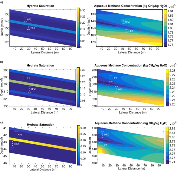
Through 1-D simulations, we explore how sand pore size distributions, sand thickness, and burial affect the potential distribution of diffusion-driven methane hydrate accumulations in coarse-grained sands. In 2-D and 3-D, we then demonstrate how hydrate growth patterns can depend on multiple sand layer interac- tions as well as concentration gradients in multiple dimensions due to sand dip.
We simulate the growth and dissociation of a hydrate-bearing sand layer buried through the GHSZ over geologic time in a Terrebonne Basin-like gas hydrate system, in which a thick,2 km water column and a low geothermal gradient contribute to a thick GHSZ. Methanogenesis properties and environmental param- eters used in this work are summarized in Table 1. Although the parameters governing rates of methano- genesis at Walker Ridge are not well constrained, we select values of the reaction rate of methanogenesis,k, and the organic carbon content at the SMT, aSMT, following Malinverno[2010]; the depth of the SMT,zSMT, is estimated based on data at Keathley Canyon [Kastner et al., 2008] and Alaminos Canyon [Smith and Coffin, 2014].
In all simulations reported in this study, a binary system of sand and clay lithologies is buried through the GHSZ to a depth of 900 mbsf; sands are characterized in 1-D and 2-D simulations by pore size distributions and in 3-D by a single pore radius,rsand, defining aqueous methane solubility. In all simulations, the clays are described by a single pore radius (rc,maxin 1-D and 2-D, andrclayin 3-D), and microbial methano- genesis is only active in the clay lithology.
3.1. One-Dimensional Lagrangian Simulations One-dimensional simulations were performed in this study to resolve at high vertical resolution the potential hydrate distribution patterns within thin sands buried through the GHSZ.
3.1.1. Pore Size Distribution Effects on Gas Hydrate Growth in Sands
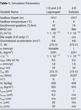
Within a single horizontal sand layer, the distri- bution of pore sizes can exert significant control on the possible distribution of hydrate through- out the sand. If there is no significant change in solubility within the layer, hydrate forms only at the sand’s edges [Rempel, 2011]. When incorpo- rating pore size distribution effects, aqueous methane solubility is reformulated additionally as a function of hydrate saturation. Thus, as hydrate forms on the edges of a sand layer, a gradient in solubility within the sand layer itself favors hydrate formation away from the sand’s edges (Figure 4).
Table 1.Simulation Parameters
Variable Name
1-D and 2-D Lagrangian
3-D Eulerian
Seafloor Depth (m) 1917 1917
Seafloor temperature (8C) 4 4
Geothermal gradient (8C/km) 19 19
BHSZ (m) 900 900
Ds(m2/s) 1310210 1310210
Dip angle (2-D only) (8) 10 n/a
Gravitational acceleration (m/s2) 9.8 9.8
Tf (K) 273.15 273.15
vf(mm/yr) Variable 1
ka(kg/m3) 2241 2241
k(s21) 1310213 1310212
aSMT(dry wt %) 0.5 0.5
x(mm/yr) 1.0 1.0
zSMT(m) 10 10
Tmb(K) 273.15 273.15
rhl(N/m) 0.027 0.027
h(8) 0 0
Hf(kJ/kg) 439 439
qh(kg/m3) 925 925
rsand(lm) n/a 1
rcmax(lm) 0.2 n/a
rclay(lm) n/a 0.01
rr(lm) 20 n/a
rm(lm) 20 n/a
Since hydrate tends to be present as a fracture-fill in fine-grained sediments, we interpret simulated hydrate saturations in the bounding fine-grained material as fracture filling. If solubility in the fine- grained sediment is lowest in the largest pores, and if no pores can fill with interstitial hydrate, then fracture-filled hydrate growth should be governed by the methane solubility of the largest clay pore.
Thus, we define a maximum pore size governing hydrate growth in the clay intervals,rc,max.
As is depicted in Figure 4, the distribution of gas hydrate within a thin sand depends heavily on the sand’s pore size distribution. If the sand exhibits a low standard deviation in pore size (Figures 4a and 4c), gas
Depth (mbsf)
270
280
290
300 310
σr = 100nm Hydrate Saturation
Depth (mbsf)
270 280
290
300 310
Hydrate Saturation σr = 10nm
Sh
r (nm)
350 400 450 500 550 600 650 700
σ = 10nm σ = 100nm
0.1 0.2 0.3 0.4 0.5 0.6 0.7
0 0.8 0.9 1.0
rm = 500nm
Depth (mbsf)
270 280
290
300 310
σr = 1 micron Hydrate Saturation
Depth (mbsf)
270
280
290
300
3100 0.1 0.2 0.3 0.4 0.5 0.6 0.70.8 σr = 100nm
Sh
r (microns)
3.5 4.0 4.5 5.0 5.5 6.0 6.5 7.0
σ = 100nm σ = 1 micron
0.1 0.2 0.3 0.4 0.5 0.6 0.7
0 0.8 0.9 1.0
rm = 5 microns
0.9 1.0
Hydrate Saturation 0.1 0.2 0.3 0.4 0.5 0.6 0.7
0 0.8 0.9 1.0
a)
b)
c)
d)
0.1 0.2 0.3 0.4 0.5 0.6 0.7 0.8 0.9 1.0 0
0.1 0.2 0.3 0.4 0.5 0.6 0.7 0.8 0.9 1.0 0
Figure 4.(left) Effective pore radius as a function of hydrate saturation, for various pore size distributions. (right) The gas hydrate distribution impact within a thin sand under four pore size distribution scenarios: (a) low median pore size and low standard deviation in pore size; (b) low median pore size and high pore size standard deviation; (c) high median pore size and low standard deviation; (d) high median pore size and high standard deviation.
hydrate is unable to accumulate in massive quantities at the center of the sand because the effective aque- ous methane solubility is nearly constant within the sand; hydrate growth in a sand characterized by larger pores (Figure 4d) fills with greater amounts of hydrate (nearly 100% of the pore space) at the sand’s edges.
Contrastingly, in a sand layer characterized by a broad pore size distribution and a relatively low median pore size closer to that of a silty lithology (Figure 4b), hydrate growth toward the center of the sand can reach upward of 20% of the average saturation at the layer’s edges. This is not possible, however, in a sand containing entirely large pores (Figure 4d). These results suggest that although a strong sand-clay solubility contrast is required to drive significant diffusive flux of methane from clays to sands, gas hydrate cannot evenly distribute throughout the sand layer unless there exists a significant gradient in aqueous methane solubility within the sand layer itself.
3.1.2. Burial Effects on Gas Hydrate Distribution Patterns in Sands
Since the rate of change in hydrate saturation within a sand grid block depends on the dissolved methane concentration gradient and inversely on grid discretization [Rempel, 2011], we impose a lognormal pore size distribution whose median pore size is determined experimentally [Bihani et al., 2015] but whose pore size at 99.7% hydrate saturation is equivalent torc,max. This ensures that as hydrate saturation increases in the sand layer, the gradient in methane concentration between the sand and surrounding clay tends toward zero, imposing a limit on the rate at which hydrate saturations can increase via diffusive methane transport.
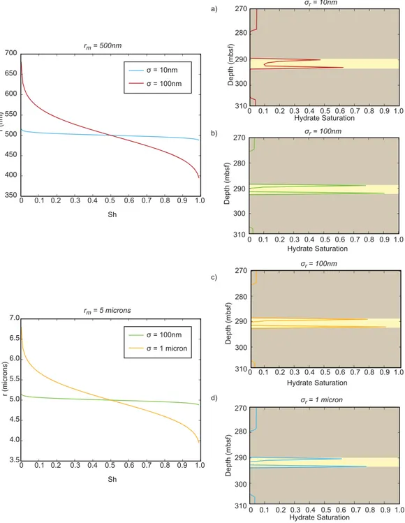
Figure 5 depicts a schematic of a 1-D simulation alongside simulated hydrate saturations in which one thin sand layer (3.6 m thick) is buried through a microbially active GHSZ at a constant sedimentation velocity, vsed(1 mm/yr in these simulations).
As shown in Figure 5, in a microbially active gas hydrate system with only compaction-driven upward fluid flow, a thin sand layer tends to diffusively soak up methane from surrounding clay material as it is buried.
The sand-clay solubility contrast promotes diffusive methane transport to the sand layer; the presence of this discontinuity requires that hydrate-free zones separate a hydrate-bearing sand from hydrate-bearing clay above and below it. Hydrate saturations in the sand layer tend to increase over time while the supply of methane via microbial methanogenesis in the clays outpaces hydrate dissolution due to increasing solu- bility with burial. Once the input of methane from microbial activity diminishes such that there is net hydrate dissolution in the bounding clays, hydrate growth is still possible in sands until all the hydrate in the surrounding clay material has dissolved.
Hydrate Saturation
t1=100ka
t2=220ka
t3=320ka
t4=615ka vsed=1mm/yr
Hydrate Saturation (fraction of pore space)
Depth (mbsf)
t5=700ka
t6=860ka
0
100
200
300
400
500
600
700
800
900
0 0.2 0.4 0.6 0.8 1
t1
t2
t3
t4
t5
t6
0 0.2 0.4 0.6 0.8 1.0 215
225
Hydrate Saturation
Depth (mbsf)
0 0.2 0.4 0.6 0.8 1.0
Hydrate Saturation
695
Depth (mbsf)705
Figure 5.One-dimensional time series evolution of hydrate saturation profiles within a single thin sand layer (3.6 m thick) in a Lagrangian reference frame as it is buried through the hydrate stability zone, incorporating capillary effects on aqueous methane concentration gradients.
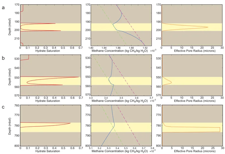
Figure 6 highlights three observable trends in gas hydrate growth patterns within a sand layer (6 m thick) as it is buried through the GHSZ. At early time (Figure 6a), hydrate is present in clays above and below the sand layer. The gradient in aqueous methane concentration is fixed by the effective solubility of methane in pore water above and below the hydrate-free zones, and diffusive methane transport is directed entirely toward the sand layer. Hydrate accumulates at a faster rate at the base of the sand than at the top. This is due to a steeper sand-clay solubility gradient at the bottom of the sand (as evidenced by the aqueous methane concentration gradients through the hydrate-free zones) as well as upward advective compaction flux. As hydrate saturations increase at the edges of the sand, the effective sand pore radius decreases and a diffusive gradient within the sand allows for methane transport toward the sand’s center.
Once the influx of microbial methane is insufficient to cause further hydrate growth in the clay layer, hydrate contained within the clay beneath the sand layer first begins to dissolve. Because hydrate is still present in the clay, however, an aqueous methane concentration gradient between the bounding clay and the sand layer still exists, so gas hydrate dissolving in the clay layer feeds hydrate that is present in the sand, preserving hydrate in the sand from dissolution with burial.
Once all of the hydrate in the clay beneath the sand layer has dissolved (Figure 6b), hydrate begins to dis- solve from the bottom of the sand layer. Although a methane concentration gradient drives diffusive flux out of the base of the sand, a concentration gradient also drives diffusive methane transport from the base of the sand to its center. Net methane migration from above is still directed toward the center of the sand.
Hydrate growth can therefore still occur at the top of the sand layer if hydrate still exists in the bounding
Hydrate Saturation
Depth (mbsf)
Methane Concentration (kg CH4/kg H2O) × 10-3 Effective Pore Radius (microns) 170
180 190
a
b
c
Hydrate Saturation 0
Depth (mbsf)
0.1
Methane Concentration (kg CH4/kg H2O) × 10-3
3.3 3.4 3.5 3.7
Effective Pore Radius (microns) 530
540 550 560
0.2 0.3 0.4 0.5 0.6 0.7
Hydrate Saturation
Depth (mbsf)
Methane Concentration (kg CH4/kg H2O) 5.1 5.2
Effective Pore Radius (microns)
0 5 10 15 20 25 30
760 770
× 10-3 200
1.80 1.84 1.86 1.88 1.92
570
530 540 550 560 570
3.6
530 540 550 560 570
780 790
800
760 770
780 790
800
760 770
780 790
800
5.3 5.4 5.5 5.6 5.7 5.8
210
170 180 190 200 210
170 180 190 200 210
0 5 10 15 20 25 30
0 5 10 15 20 25 30
0 0.1 0.2 0.3 0.4 0.5 0.6 0.7
0 0.1 0.2 0.3 0.4 0.5 0.6 0.7
Figure 6.Patterns of gas hydrate distribution (red), dissolved methane concentration (blue), and effective pore radius (orange) governing effective methane solubility within a 6 m thick sand layer as it is buried through the GHSZ (a) early in burial, (b) at an intermediate burial depth, and (c) late in burial. A dashed green line indicates free space bulk aqueous methane solubility, and a dashed magenta line indicates the effective aqueous methane solubility in clay pores. The sand layer is highlighted in yellow, and the bounding clay is highlighted in brown.
clay above the sand (or as long as the methane concentration in this region exceeds the solubility of meth- ane in the pore water of the sand). Once the hydrate within the clay above the sand and at the base of the sand fully dissolves (Figure 6c), hydrate on the upper sand boundary proceeds to dissolve. In this case, the methane concentration gradient drives diffusive methane transport out of the sand from above and below.
It is important to note that the gas hydrate distribution patterns shown here reflect the potential trends in diffusion-driven methane hydrate growth and distribution in sand layers. These patterns depend on how rapidly methane generation decreases with depth and on the initial conditions of the simulation at the time of sand deposition. In the simulations performed here, no methane is initially present at the SMT at the time of deposition of the modeled sand layer. The results of these simulations therefore correspond to the maximum rate at which hydrate dissolution should take place. If methane is present in the system as an ini- tial condition or if the rate of methane generation decreases more slowly with depth than in these simula- tions, the hydrate distribution pattern illustrated in Figure 6a might be preserved with deeper burial. In certain instances where there is significant methane sourcing at depth in the GHSZ, the system may never exhibit the patterns described in Figures 6b and 6c.
Intriguingly, these simulations illustrate the potential for gas hydrate dissolving within clay over time to feed and preserve the hydrate existing within sand layers against dissolution while burial increases aqueous methane solubility. This suggests that if hydrate deposits are observed to occur in any quantity within clays at depth in close proximity to thin sands, hydrate grown in the sands could have been preserved during burial as the sands soaked up methane from dissolving hydrate in clays.
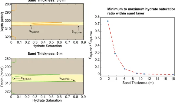
3.1.3. Sand Layer Thickness Effects on Gas Hydrate Distributions Within a Sand
For a given pore size distribution within a sand layer, the distribution of gas hydrate within a coarse-grained sand layer depends on the sand layer thickness, all else remaining constant. Figure 7 compares the accumu- lation of gas hydrate within a sand layer at a particular depth for different sand thicknesses, holding con- stant the grid discretization and the amount of methane generated through microbial methanogenesis in the bounding clays.
For small sand thicknesses (the 3.6 m sand in Figure 7), the aqueous methane concentration gradient between a sand’s edge and its center is stronger than that in a thick sand because of the shorter distance over which methane must travel for a given contrast in solubility. The ratio of the minimum to maximum hydrate saturation within a sand (Figure 7) therefore decreases with increasing thickness and eventually reaches 0 at a finite sand thickness. Furthermore, simulations indicate that the average hydrate saturation
10 12 14 16 18 0
0.1 0.2 0.3 0.4 0.5 0.6 0.7 0.8
8 6 4 2 0
Sand Thickness (m) Shyd,min / Shyd,max
280 290 300 310 320
Hydrate Saturation
0 0.1 0.2 0.3 0.4 0.5 0.6 0.7 0.8 0.9
Depth (mbsf)
280 290 300 310 320
Hydrate Saturation
0 0.1 0.2 0.3 0.4 0.5 0.6 0.7 0.8 0.9
Depth (mbsf)
Sand Thickness: 9 m Sand Thickness: 3.6 m
Minimum to maximum hydrate saturation ratio within sand layer
Shyd,min Shyd,max
Shyd,min Shyd,max
Figure 7.A comparison of minimum to maximum hydrate saturation within a sand for varying thicknesses of sand layers bounded by clays. The sand layer is highlighted in yellow, and the clays are highlighted in brown.