Geochemistry,Geophysics,Geosystems PUBLICATIONS

(1)

RESEARCH ARTICLE

10.1002/2017GC006805

Observed correlation between the depth to base and top of gas hydrate occurrence from review of global drilling data

M. Riedel¹ and T. S. Collett²

1GEOMAR Helmholtz Centre for Ocean Research Kiel, Kiel, Germany,²US Geological Survey, Denver Federal Centre, Denver, Colorado, USA

Abstract

A global inventory of data from gas hydrate drilling expeditions is used to develop relationships between the base of structure I gas hydrate stability, top of gas hydrate occurrence, sulfate-methane transition depth, pressure (water depth), and geothermal gradients. The motivation of this study is to provide ﬁrst-order estimates of the top of gas hydrate occurrence and associated thickness of the gas hydrate occurrence zone for climate-change scenarios, global carbon budget analyses, or gas hydrate resource assessments. Results from publically available drilling campaigns (21 expeditions and 52 drill sites) off Casca- dia, Blake Ridge, India, Korea, South China Sea, Japan, Chile, Peru, Costa Rica, Gulf of Mexico, and Borneo reveal a ﬁrst-order linear relationship between the depth to the top and base of gas hydrate occurrence.

The reason for these nearly linear relationships is believed to be the strong pressure and temperature dependence of methane solubility in the absence of large difference in thermal gradients between the various sites assessed. In addition, a statistically robust relationship was deﬁned between the thickness of the gas hydrate occurrence zone and the base of gas hydrate stability (in meters below seaﬂoor). The relationship developed is able to predict the depth of the top of gas hydrate occurrence zone using observed depths of the base of gas hydrate stability within less than 50 m at most locations examined in this study.

No clear correlation of the depth to the top and base of gas hydrate occurrences with geothermal gradient and sulfate-methane transition depth was identiﬁed.

1. Introduction

Over the past two decades, numerous marine drilling expeditions were conducted to study gas hydrate occurrences, specifically with an aim to understand the geologic controls on the occurrence of gas hydrate and to understand their role as a future source of energy. Deep scientific drilling was performed on the southern and northern Cascadia margin, off India, China, Japan, South Korea, the eastern U.S. margin (Blake Ridge), and the U.S. Gulf of Mexico. The aim of our study presented here is to define (if present) first-order correlations between the top of gas hydrate occurrence zone (TGHOZ), base of gas hydrate stability zone (BGHSZ), and possibly any further correlations with the depth of the sulfate-methane transition zone (SMTZ), and derived geothermal gradients. To do so, we compiled data from 21 deep drilling expeditions (see details below). Some earlier attempts in combining such information is provided inBooth et al. [1996]

or the compilation by the US Geological Survey [e.g.,Kvenvolden and Lorenson, 2001].

In addition to the study of gas hydrates from an energy point of view, defining the global abundance of gas hydrate is also important to estimate their potential as natural hazards (to production or the environment) as well as for climate studies. In this context, the top of gas hydrate occurrence and the base of gas hydrate stability define the container size required to estimate the resource potential and thus the total amount of carbon stored in solid gas hydrates. The vulnerability of gas hydrate to climate change (e.g., a warming scenario) is linked to the overall burial depth below seafloor and overall water depth of the gas hydrate occurrence. The depth to which gas hydrate occurs in the sediment is further controlled by the geothermal gradient and methane concentrations in sediment pore waters at depth (see schematic diagram in Figure 1). Our compilation of deep drilling data, especially the top of gas hydrate occurrences as observed in core and log-data, may also be a useful asset for developing future gas hydrate drilling campaigns, especially with depth-limited devises such as seafloor drill rigs, or in regions where no previous drilling information on the extent of gas hydrates occurrences exist, and information about gas hydrates may be limited to seismic observations of a bottom-simulating reflector (BSR) as main indicator for the simple presence of gas hydrates in that region.

Key Points:

An inventory of 21 gas hydrate drilling campaigns is presented

The top of gas hydrate occurrence and depth of gas hydrate stability are deﬁned from drilling with

uncertainties depending on proxy used

Statistical relationships are developed to predict thickness of gas hydrate occurrence zone from depths of gas hydrate stability

Correspondence to:

M. Riedel, mriedel@geomar.de

Citation:

Riedel, M., and T. S. Collett (2017), Observed correlation between the depth to base and top of gas hydrate occurrence from review of global drilling data,Geochem. Geophys.

Geosyst.,18, 2543–2561, doi:10.1002/

2017GC006805.

Received 6 JAN 2017 Accepted 1 JUN 2017

Accepted article online 9 JUN 2017 Published online 13 JUL 2017

VC2017. American Geophysical Union.

Geochemistry, Geophysics, Geosystems

PUBLICATIONS

(2)

The balance between pore water methane solubility (itself a function of temperature and pressure) and local methane concentrations is a critical factor in allowing the formation of gas hydrate, and local methane concentrations are influenced by in situ methane production (a function of total organic carbon available, as well as temperature), methane advection by fluid flow from greater depth, and sedimentation (burial) rates. Several authors have estimated the global abundance of gas hydrates [e.g.,Kvenvolden, 1988;Milkov, 2003;Klauda and Sandler, 2005] or more local basin wide estimates (e.g., for the U.S. Gulf of Mexico by the Minerals Management Service[2008]) but global estimates vary over several orders of magnitude. Also, assessments conducted for energy assessments are not always directly comparable to those made for global methane abundance and climate studies (though technically mostly based on the same overall methodology) as described inBoswell and Collett[2011].

Other approaches for predicting gas hydrate abundance have been suggested, e.g., based on geochemical transport-reaction modeling [e.g.,Wallmann et al., 2006], transfer functions based on measured pore fluid compositions [e.g.,Marquardt et al., 2010] or coupled momentum, mass, and energy equations [e.g.,Xu and Ruppel, 1999]. In all these analyses, either complex mathematical modeling needs to be performed or downhole pore fluid observations are required as verification of predicted concentrations. Several attempts have been previously suggested to calculate the vertical abundance of gas hydrate from the depth of the SMTZ and the shape of the down-core profiles of sulfate (and methane), as described, e.g., byPaull et al. [2005]

andBhatnagar et al. [2008, 2011]. Here data from shallow (piston/gravity) coring are used. The issues associated with these approaches are often impacted by a number of factors, including the limited nature of the gas being sourced mostly by microbial processes, controls on vertical (1-D) ﬂuid migration, lack of incorpo- ration of sediment-type controls on hydrate growth, and difﬁculties in the calibration of model-results with available drilling/core data.

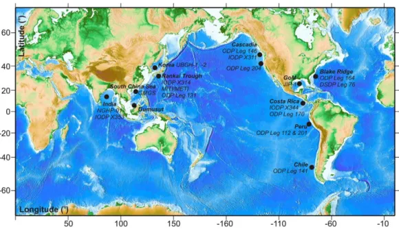
In contrast, it may be possible to deﬁne a simpler approach to set critical boundaries to the potential size of the ‘‘gas hydrate stability container’’ (i.e., top and base of the stability ﬁeld) if one can develop empirical relationships for these parameters from deep drilling observations. In order to investigate if such correlations may exist and how robust these may be, we have compiled data from 58 individual drill sites completed as part of 21 drilling campaigns in ten different geological regions, for which coring and/or geophysical logging programs were conducted (Figure 2).

The following drilling sites and margins were included in this study:

1. Cascadia Margin (active continental margin, accretionary prism):

i. Ocean Drilling Program (ODP) Leg 146 [Westbrook et al., 1994],

ii. Integrated Ocean Drilling Program (IODP) Expedition 311 [Riedel et al., 2006], and iii. ODP Leg 204 [Trehu et al., 2003].

Figure 1.Schematic diagram for (a) gas hydrate phase boundary and (b) methane concentration (green dashed and black dotted lines are two simplified examples) and methane solubility. Identified are the depths of the sulfate-methane transition zone, top and base of gas hydrate stability zone, as well as the corresponding top and base of gas hydrate occurrence zone (TGHOZ, BGHOZ) for the two examples of methane concentration profiles. Depth is not plotted to scale.

(3)

2. Blake Ridge (passive continental margin) i. ODP Leg 164 [Paull et al., 1996] and ii. DSDP Leg 76, Site 533 [Sheridan et al., 1983].

3. India East Coast (passive continental margin)

i. India National Gas Hydrate Program Expedition 1, NGHP-01 [Collett et al., 2014;Kumar et al., 2014, and references therein] and

ii. IODP Expedition 353, Sites U1445 and U1446 [Clemens et al., 2016].

4. Korea (back-arc basin)

i. Ulleung Basin Gas Hydrate Drilling Program, UBGH-1 and22 [Park et al., 2008;Ryu et al., 2013, and references therein].

5. Costa Rica Margin (active continental margin, erosive sedimentary prism) i. IODP Expedition 344, Site U1412 [Harris et al., 2013] and

ii. ODP Leg 170 [Kimura et al., 1997].

6. Borneo (passive continental margin)

i. Gumusut drilling project [Paganoni et al., 2016].

7. Peru (active continental margin, accretionary prism) i. ODP Leg 201, Site 1230 [D’Hondt et al., 2003] and ii. ODP Leg 112, Sites 685 and 688 [Suess et al., 1988].

8. Gulf of Mexico (passive continental margin)

i. Joint Industry Project, Keathley Canyon KC151 [Ruppel et al., 2008, and references therein].

9. South China Sea (passive continental margin)

i. Sites SH-2, 23, and 27 [e.g., Matsumoto et al., 2011, and references therein; Wang et al., 2011a, 2011b, 2014a, 2014b;Wu et al., 2011].

10. Japan, Nankai Trough (active continental margin, accretionary prism) i. ODP Leg 131, Site 808 [Taira et al., 1991],

ii. MITI Wells [Tsuji et al., 2004;Matsumoto, 2008],

iii. METI Wells,a-1 andb-1 well [Takeuchi and Matsumoto, 2009], and iv. IODP Expedition 314, Site C0002 [Miyakawa et al., 2014].

11. Chile (active continental margin, erosive prism

i. ODP Leg 141, Sites 859, 860, and 861 [Behrmann et al., 1992].

It is important to note that coring operations with modern detection techniques such as infrared (IR) core imaging, which has been used since ODP Leg 201 [Ford et al., 2003] and ODP Leg 204 [Weinberger et al., 2005]

Figure 2.Map showing generalized locations of drilling campaigns utilized in this study. In each region, several drill sites are considered.

For details, refer to Table 1 and references cited in text.

(4)

have allowed more careful analyses of sites cored in the past15 years compared to earlier such undertak- ings. When discussing statistical relationships between depths of gas hydrate occurrences and other parameters (as outlined below), the relative vintage of the data from expeditions conducted during earlier drilling campaigns such as DSDP Leg 76 [Sheridan et al., 1983] and ODP Leg 112 [Suess et al., 1988] should be considered with an overall larger degree of uncertainty (as discussed later).

In the context of this study, we strictly use the structure I gas hydrate phase boundary and ignore occurrences of higher hydrocarbons that may generate structure II gas hydrates. Thus, the term BGHSZ is to be interpreted as base of structure I gas hydrate, or in line with previous suggested terminology, BS_IGHSZ [e.g., Boswell et al., 2016;Paganoni et al., 2016]. We further want to emphasize that our study is not concerning the detailed and local gas hydrate concentrations with depth and any localized variations therein. As the drilling of gas hydrate over the past decades has shown a high degree of intrasite variability (e.g., during ODP Leg 204 [Trehu et al., 2004] or IODP Expedition 311 [Riedel et al., 2006]) such details are not considered for this study.

2. Data, Methods, and Uncertainties

The detection of gas hydrate can be made either directly through visual observations of the core or by indi- rect observations and the use of proxy measurements as compiled inRiedel et al. [2010]. Data used for our inventory are from offshore drilling campaigns that span the time from as early as 1983 with DSDP Leg 76 [Sheridan et al., 1983] to IODP Expedition 353 off India conducted in 2015 [Clemens et al., 2016]. The proxies used in this study include core-based proxies such as pore water freshening in the form of reduced chlorinity as shown in Figure 3a and described first byHesse and Harrison[1981], significant cold spots in IR images of cores just after recovery (Figure 3b) [e.g.,Long et al., 2010], soupy or mousse-like textures of sediments [e.g.,Kastner et al., 1995;Pinero et al., 2007] (Figure 3b), logging-based proxies compiled byCollett and Lee [2012] such as formation-responses above a (site-specific) background trend in either electrical resistivity (Figure 3c),PandSwave velocity, or sonic wave attenuation or pressure-core-derived methane concentrations (Figure 3d) [Schultheiss et al., 2010].

Log-data used in this study are either from conventional wireline (WL) deployments where data are acquired after a hole has been drilled or logging-while-drilling (LWD) techniques, where data are acquired at the same time as the hole is advanced. Differences in these two principle logging-techniques and their relevance to detecting and quantifying gas hydrates are described byCollett and Lee[2012] orGoldberg et al. [2010].

Overall, substantial differences exist between the various methods to detect gas hydrate and each method bears its own uncertainty. Uncertainties in defining the occurrence of gas hydrate based on data from recovered sediment cores is often challenged by the quality of the recovered cores and the extent of core coverage over the depth interval of interest. Incomplete core recovery, spot-coring approaches, core- expansion after recovery from sediment pore water degassing (often augmented by gas hydrate dissociation during core recovery) all lead to a significant uncertainty in assigning depth values to acquired core measurements. Prior to the use of IR-guided core sampling to identify cold spots associated with dissociat- ing gas hydrate, pore fluid-based detection of gas hydrate was purely a hit-and-miss undertaking. The presence of gas hydrate can be inferred through observations of the core and using typical textures as proxies (soupy or mouse-like sediment disturbances). Thus, only continuous coring and exploitation of all core- based proxies can lead to a robust definition of the top of gas hydrate occurrence zone. However, the time gap between core recovery, examination in the core recovery lab, and IR scanning can influence the detection of gas hydrate [Weinberger et al., 2005]. Moreover, if a gas hydrate occurs close to the center of the core, the IR cold spot anomaly may only be seen after some additional time has lapsed to allow for more complete hydrate dissociation and associated conduction of the temperature anomaly to reach the outer core liner, where it can be imaged with the IR camera. Here secondary scans and/or comparisons with core- textures may help to better infer the presence of gas hydrates [Long et al., 2010]. However, the lower limit of the ability of IR scanning (or the development of significant disturbed sediment textures) to detect gas hydrate dissociation is not known and is largely dependent on the experience of the individual(s) perform- ing the analysis as well as and ambient conditions during the IR scanning (such as outside air temperature, sun light conditions, humidity, core-liner material, and handling of the core prior to scanning).

(5)

Using logging-based proxies in defining the occurrence of gas hydrates also holds a variety of uncertainties, including the nature of the physical measurement made by the logging tool and its ability to provide robust measures for detecting gas hydrate, the logging-technique (LWD or WL), speed of logging, borehole conditions, logging tools, and drilling-fluid used. Ship heave-compensation is usually robust enough to compen- sate for any ship-motion, so depth uncertainties associated with downhole log-data are generally rare and are usually associated with the selection and/or use of an incorrect reference datum such as inaccurately picking the depth of the seafloor from the acquired logs. In general, the vertical resolution of WL tools is higher (few centimeters) than LWD tools (tens of centimeters), but for the most part both logging- techniques yield relatively high resolution analysis of the occurrence of gas hydrate. By comparison, LWD data can be acquired from the seafloor to the bottom of the drilled hole, but WL data cannot usually be obtained from the upper 30–90 m of each well logged because of borehole stability problems; thus, limiting

Figure 3.Examples of determining gas hydrate occurrence from (a) pore water chlorinity freshening and (b) core-IR imaging in combination with soupy and/or mouse-like sediment textures, (c) log-data responses using electrical resistivity anomalies relative to background as the main indicator for the presence of gas hydrate with Figure 3d, supporting evidence from pressure-core-derived gas hydrate concentrations. Also shown are the core recovery plots to show how incomplete core recovery may hamper deﬁnition of top and base of gas hydrate occurrence from core-based data. Deﬁnition of the depth of the sulfate-methane transition zone (SMTZ) from sulfate and methane data is shown in Figure 3e. All images are based on data from Site U1326, IODP Expedition 311 [Riedel et al., 2006].

(6)

Table1.GlobalDataBaseofDrilling-DerivedValuesinTopofGasHydrateOccurrenceZone(TGHOZ),BaseofGasHydrateStabilityZone(BGHSZ),Sulfate-MethaneTransitionZone(SMTZ)andGeothermalGradientsa Site LocationSMTZ (mbsf)TGHOZ (mbsf)BGHSZ (mbsf) Water Depth (m)b

Thermal Gradient (8C/km)BGHSZ (mbsl)TGHOZ (mbsl) Thickness GHOZ (m)

PredictedTGHOZ (mbsf)Difference(m) ReferenceEquation (1)Equation (2)Equation (1)Equation (2) CascadiaMargin IODPX311 13254.5617365c(Cl–)245617d2201616063244661822746617262286.4138.813.433.7Riedeletal.[2006,2010] 13262.5614761e(Cl–)26162d182861n.d.20896318756221463117.2150.170.263.9 132786111161(LWDres.)23068d132261556415526914336211969108.4127.222.628.2 1329961n.d.12563d960617264108564n.d.n.d.n.d.n.d. ODPLeg204 12448.5614561e(IR,Cl–)1256390761606110326495262806425.049.8220.030.2Trehu

etal.[2003] 12467614061e(IR,Cl–)114628606161629746390062746316.441.7223.632.3 124712614561e(IR,Cl–)122638456152619676489062776424.747.6220.329.4 12514.5619061e(IR,Cl–)197.56512206153611420661310621106683.9105.126.14.9 12457615161e(IR,Cl–)13667.8880615561101468.8931628368.834.756.4216.326.6 12525614361e(IR,Cl–)1706510406159641210661083621276662.683.019.644.0 BlakeRidge ODPLeg164 99420.56119561.5f(Cl–)4286527986136.461.3323666299362.523366.5237.1273.242.1240.2Paulletal.[1996] 995216119061.5f(Cl–)4506102777.76133.560.93238611297862.5260611.5258.6289.468.6229.4 997236121061.5f(Cl–)4516827706136.461.3322169298062.524169.5260.3290.150.3249.1 DSDP 5332265g24764h6006531916136.0i37916634386535369385.7400.0138.7247.0Sheridanetal.[1983] India NGHP-1 1–3106116562f(IR,Cl–)200651076613962127666124163356789.9105.1275.1270.1Collettetal.[2014]and referencestherein1–5216170.464f(Cl–)1306494561446310756510176556.66828.253.5242.26.1 1–732616161(LWDres.)193.56512856152621478.566134662132.56675.0100.314.032.2 1–1422615264f(Cl–)129.5620j8956138621024.56219476577.5624j29.853.1222.224.4 1–17256126061f(IR,Cl–)61466134461196219586716046235467475.6410.3215.6256.3 1–18206111261f(IR,mous.)21562.51374615062k158963.514866210363.591.9116.1220.1213.1 1–1921619868f(Cl–)19567.51422615362161768.515206997615.570.7101.4227.324.4 1–2014614561f(IR,Cl–)195615j1146614962k134161611916215061682.2101.437.248.6 1–6n.d.11061f(IR,Cl–)21065116061n.d.137012701006696.0112.5214.0212.5 1–4n.d.8061(LWDres.)18265108161n.d.1263661161621026672.491.827.610.2 1–2n.d.5861(LWDres.)17065105861n.d.1228661116621126661.883.03.829.0 1–8n.d.n.d.25765168961n.d.194666n.d.n.d.n.d.n.d. 1–9n.d.n.d.29065194661n.d.223666n.d.n.d.n.d.n.d. X353 144517613161f(IR,Cl–)n.d.2502615062kn.d.253362n.d.n.d.n.d.Clemensetal.[2016] 1446206112561f(IR,Cl–)247.567.5l1430615062k1677.568.5155562122.568.5120.790.32116.2265.3 Korea UBGH 2–1_17.7619461f(IR,Cl–)16562j15346110062k169963162862716337.379.3256.728.3Ryuetal.[2013]and Bahketal.[2013]2–1_2n.d.7061f(LWDres.)16565l149861Assumed166366156862956638.879.3231.215.7 2–4n.d.14061f(LWDres.)18365l215661Assumed233966229662436628.892.62111.2249.6 2–66.56111261f(IR,Cl–)172.562.521526111262k232263.52264625863.516.583.0295.5225.0 2–8n.d.7561f(LWDres.)16565l198861Assumed2153662063906618.579.3256.510.7 2–96.7619561(LWDres.)1646521066111562k22666622016265668.975.6286.1210.6 2–58.2614061f(IR)184631974619662k2158642014621446437.393.322.750.7 1–4n.d.15561f(IR,Cl–)18065l184561Assumed2025662000256638.890.32116.2265.3Parketal.[2008] Borneo/Gumusut DC_En.k.10561f(Cl–)15565948.5616362k1103.5661053.562506652.071.9253.0221.9Paganonietal.[2016] SouthChinaSea SH-7176113561f(Cl–)18163110561n.k.128364124062436467.688.9267.4245.9Wangetal.[2011a,b,a,b] andWuetal.[2011]SH-2256118561f(Cl–)251617j12306145.662k147561814156260618126.6138.3258.4278.3 SH-322617061f(Cl–)20662124061n.k.1446631310631366388.8109.518.826.5 JapanNankaiTrough Alpha-1236110061f(Cl–)2006273061n.k.930638306210063104.24.2105.125.1TakeuchiandMatsumoto [2009]Beta-176110560.5f(Cl–)33762997614362k133463110261.523262.5224.5119.5206.125.9 MITIWell1n.d.17561f26861945614362k1213621141629362160.5214.5155.2262.2Matsumoto[2008] C0002(X314)n.k.220610m(LWDres.)4006101964615062k23646112184611180620244.824.8252.5272.5Miyakawaetal.[2014]

(7)

Table1.(continued) Site LocationSMTZ (mbsf)TGHOZ (mbsf)BGHSZ (mbsf) Water Depth (m)b

Thermal Gradient (8C/km)BGHSZ (mbsl)TGHOZ (mbsl) Thickness GHOZ (m)

PredictedTGHOZ (mbsf)Difference(m) ReferenceEquation (1)Equation (2)Equation (1)Equation (2) Site8081061110625n205610484161111.66105046611495162695635261.3261.3108.8213.8Tairaetal.[1991] GoM-JIP1 KC151#2106110061f(Cl–,LWDres.)392621321.861n.k.1713.8631421.86229263263.7246.6163.745.4Ruppeletal.[2008]andrefer- encestherein CostaRica IODPX344 141214.76171.661f(Cl–)187651921618562k(1148)210862199262115.46242.495.5229.219.9Harrisetal.[2013] Leg170 104020629065f(Cl–)n.d.4177617.262kn.d.426766n.d.n.d.n.d.Kimuraetal.[1997] 10411562116.765f(Cl–)n.d.3317612262kn.d.3433.766n.d.n.d.n.d. Peru ODPLeg201 123086171.663f(Cl–)610650j50866134.362k5696651515964537653316.8243.8407.3129.7D’Hondtetal.[2003] ODPLeg112 685126299620f610650j50706134.362k56806515169621511670317.5218.5407.3103.7Suessetal.[1988] 6881062135620f500650j3820615262k43206513955621365670263.8326.3128.838.7 682n.d.n.d.477650j3790614962k4267651n/an/an.d.n.d. 6831662n.d.n.d.3072615062kn/an/an/an.d.n.d. Chile ODPLeg141 859<5i30610f(Cl–)8061027416219062k2821612277161150620294.116.62124.133.4Behrmannetal.[1992] 860<10in.d.158610232062106.462k2478612n.d.n.d.n.d.n.d. 861<12in.d.25062016586253.5in.d.n.d.n.d.n.d. aAlsoindicatedarethetypesofproxyusedfordetectiononsetofgashydrates(Cl–:porewaterchlorinityfreshening,IR:infraredimaging,mous.:mousse-likesedimenttexture,LWDrest.:Logging-while-drillingresistivity anomaly)aswellasuncertaintiesinthedepthvalues.Theseuncertaintiesareafunctionoftheproxyusedtodefinetheparametersaswellascorerecoverythroughtheintervalofhydrateoccurrences.n.d.:notdeter- minedandn.k.:notknowntoauthors. bUncertaintiesreportedareroundedtothenearestmeterandarefromdeterminingaveragevaluesfromallavailablemeasurementsatthedrillsite(whichcanincludesomeorallofdriller’sdepth,acousticdepthrang- ing,seismicdepth,orROVdive-depths). cUncertaintyisbasedonpoorcorerecoveryinthatinterval. dUncertaintyisbasedonRiedeletal.[2010,Table1],wheretheBGHSZwasdefinedfromvariousboreholemeasurements,core-analyses,thermalgradients,andseismicdata. eUncertaintyof1misusedforintervalswithgood/highcorerecovery,wheregasexpansionvoidsandsedimentextrusionresultsinupto1mdepthuncertaintypostcuration. fUncertaintyisdefinedbysamplespacing. gUncertaintyisdefinedbyrangeofobservationsgiveninTable4ofDSDPVol.76,p.61. hUncertaintyisdefinedbyrangeofobservationsgiveninTable1ofDSDPVol.76,p.48. iNouncertaintyreportedinliterature,andnonewuncertaintywasdefined. jUncertaintyfromdiscrepancybetweenthermaldataandseismicobservations. kUncertaintyassumed;onlyoneortwodatapointsacquired,sonoregressionwasattempted. lUncertaintyfromunknownvelocitytoconvertbottom-simulatingreflector(BSR)depthsfromseismicdatatodepthbelowseafloor. mUncertaintyfromabroadzoneofelevatedresistivityvaluesinLWDdata. nUncertaintyfromonerecoveredgashydratepieceinwashcore131–808F-4W. oThereportedvalueof1148C/kmbyHarrisetal.[2013]isbasedonfewvaluesintheupper35mbsf.UsingtheseismicallydefineddepthoftheBSR(190mbsf)andaseafloortemperatureof2.258C,yieldsageothermal gradientof858C/kmfortheexpectedtemperatureatthephaseboundaryasdefinedforaseawater(34ppt)andpuremethanemix.

(8)

the coverage of WL acquired log-data. Detecting gas hydrates from the formation response using logged physical properties such as electrical resistivity,PorSwave velocity, or acoustic wave attenuation, requires establishing a site-dependent background trend in these physical properties, which are a function of poros- ity, in situ pore fluid composition, and bulk density of the formation (e.g., occurrence of authigenic car- bonates). Additional influence on the ability to detect gas hydrate is the mode of occurrence (i.e., pore- filling, forming as veins, or massive nodules) and the sensitivity of the tool and measurement technique to anisotropy.

The depth of the sulfate-methane transition zone (SMTZ) in marine sediments is based on the measurement of sulfate and methane concentrations in recovered sediment core (Figure 3e). As the term SMTZ implies, this is a zone of some thickness, not necessarily

Figure 4.Correlations between geothermal gradient and (a, b) base of gas hydrate stability zone, and (c, d) top of gas hydrate occurrence (each shown in meters below seaﬂoor (mbsf) in the upper panel, and meters below sea level (mbsl) in lower panel). Data from drilling campaigns are used where the geothermal gradients were determined by in situ measurements.

Colors and symbols used in all subﬁgures are shown in the legend.

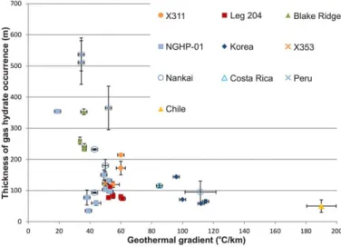
Figure 5.Crossplot of measured geothermal gradients and measured thickness of the gas hydrate occurrence zone (uncertainties see Table 1).

(9)

with a sharp boundary. We assign an uncertainty of 61 m to the depth values of SMTZ reported in Table 1, which includes the uncertainty associated with deﬁning the seaﬂoor. Using the ‘‘mud-line core’’

to define seafloor and all subse- quent depths as meters below seafloor (mbsf) can have some error usually due to the fact that the seafloor itself is not always captured in the core.

Deﬁning geothermal gradients requires reliable measurements of temperature within the sediment column and at the seaﬂoor. Data reported here from ODP and IODP drilling expeditions often utilize temperature measurements during piston coring [e.g., Heesemann et al., 2006] or by using special wireline deployed tools mechani- cally inserted into the sediments, such as the Davis-Villinger Temper- ature probe [Davis et al., 1997].

Other similar industry tools have been used during commercial drilling campaigns in the South China Sea [e.g., Wang et al., 2014a], Ulleung Basin [e.g., Ryu et al., 2013], or off Borneo [Paganoni et al., 2016]. While each individual temperature measurement may yield a highly accurate temperature value, the temperature gradient is derived from the statistical analysis of individual tool derived values.

Fundamentally, the assumption in all these regression analyses is a linear extrapolation of the geothermal gradient through the gas hydrate occurrence zone; which might not always be a correct assumption.

Uncertainties in the values reported in Table 1 may be signiﬁcant, but is not always provided with the reported data.

Overall, when comparing the ability of deﬁning the top of gas hydrate occurrence zone from core-based proxies and direct observations or log-based methods, the core-based analyses are more reliable, especially in case of continuous coring. Core-based techniques allow physical testing of samples, whereas remote sensing relies on many assumptions (e.g., physical properties for the background hydrate-

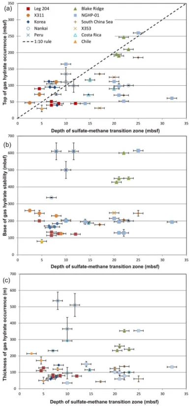
Figure 6.Correlation between the sulfate-methane transition zone depth and (a) the top of gas hydrate occurrence, (b) depth of the base of gas hydrate stability, and (c) thickness of the gas hydrate occurrence zone as measured from sites of 12 drilling campaigns (colors and symbols deﬁned in legend). Data and uncertainties for each site are reported in Table 1 (references see text).

(10)

free lithology), especially if no core was recovered, or core hole and log-hole are at considerable distance to each other. In our analyses of correlations between the depth to the top and base of gas hydrate occurrence zone with the depth of the SMTZ and geothermal gradients, the uncertainties in the derived depth values vary between sites and are listed in Table 1.

In order to obtain a robust statistical analysis of the derived depths and geothermal gradients, we have used a total least squares (TLS) analytical technique, which allows vari- able errors in both dimensions and the definition of the robustness of the linear fit to the data with uncorrelated errors [Krystek and Anton, 2007]. Uncertainties used in the TLS method are dependent on the proxy used to define gas hydrate occurrence, as well as the statistical best fit value for defining BGHSZ (when e.g., using various measures from geophysical log-data, seismic, and thermal measurements). All uncertainties are included in Table 1.

3. Results

In general, drilling campaigns provide a wealth of information on the occurrence of gas hydrates and include analysis of local and regional geologic settings such as active continental margins with accretionary prisms (Cascadia, Nankai Trough) and erosive prisms (Costa Rica, Peru), passive continental margins (South China Sea, Blake Ridge, India, Gulf of Mexico, Borneo), and back-arc basins (Korea). None of the sites included in our compilation are associated with vigorous ﬂuid ﬂux at cold vents or other recent local disturbances such as sediment slumping.

As described in section 2 above, we have selected at each site listed in Table 1 the depth to the top of gas hydrate occurrence zone (TGHOZ), depth of the SMTZ, depth to the base of gas hydrate stability zone (BGHSZ) and the calculated geothermal gradient at the site, as determined either by using the cited values in the scientific literature or by reanalyzing the available data provided through the ODP and IODP online databases. Figure 4 combines observations in the relationship between measured geothermal gradients and the depths to the TGHOZ and BGHSZ. When plotting the BGHSZ depth values as function of depth below sea level (Figure 4a) assuming hydrostatic pressure conditions or meters below seafloor (Figure 4b), no obvious correlation with the geothermal gradients is evident. Similarly, with increasing thermal gradients, the TGHOZ should become shallower as methane becomes more soluble in the pore waters with increasing temperature, assuming constant upward fluid (including dissolved gas) flux rates from below. This trend is not obviously reflected in the drilling data (Figure 4c). However, there may be suggested lower limit for the TGHOZ for any given geothermal gradient (as shown by the dashed line in Figure 4c. The thickness of the gas hydrate occurrence zone is also not strongly correlated to the geothermal gradient values but the thickness is overall reduced with higher geothermal gradients (Figure 5).

As the occurrence of gas hydrate is closely linked to the site-specific shape of the methane solubility curve with depth and available methane in the subsurface to form gas hydrate (either from in situ microbial production or in combination with advection from fluids, where methane was generated at greater depth, including thermogenic sources), an initial thought has been, that the depth of the SMTZ may be an indicator for predicting the top of the first gas hydrate occurrence as it may reflect the in situ methane fluxes [Bhatna- gar et al., 2008, 2011;Kastner et al., 2008;Dickens and Snyder, 2009;Chatterjee et al., 2009;Malinverno and Pohl- man, 2011]. An additional suggestion had been that there is a 1:10 relationship between the depths of the SMTZ and TGHOZ [Paull et al., 2005]. On the basis of the available drilling data (Figure 6), we present three crossplots between the SMTZ depth and the depth of the TGHOZ and BGHSZ, as well as the thickness of the gas hydrate occurrence zone. As can be seen in the plots in Figure 6, the scatter in the complete data set is considerable and no clear trend for the entire data set can be identified. However, if for example only a sub-

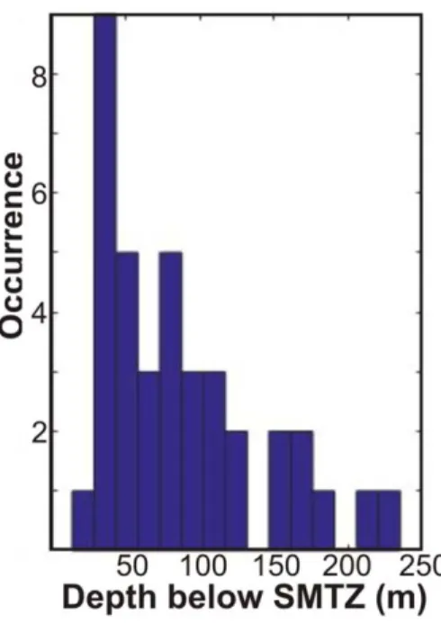
Figure 7.Distribution of the depth to the top of hydrate occurrence zone (TGHOZ) below the sulfate-methane transition zone (SMTZ) from all drilling campaigns listed in Table 1. The majority of sites show the ﬁrst gas hydrates between 40 and 50 m below the SMTZ.

(11)

set of drill sites (e.g., only those from IODP Expedition 311) are used, some trend between the SMTZ and the depth to TGHOZ becomes evident, in that for a deeper SMTZ, the depth to the TGHOZ is increased, and the BGHSZ becomes shallower.

The depth of the base of the SMTZ is often very well deﬁned through careful geochemical pore water and head-space gas analyses of core samples and the depth-uncertainty is overall small (0.5 m). Yet the uncertainty in assigning a value to the BGHSZ or TGHOZ may be as large as 10 m or even more for some of the sites from older drilling campaigns. Nonetheless, it is obvious from these data that the TGHOZ occurrence is not at the same depth as the base of the SMTZ but at some (often considerable) depth below (Figure 7). While the depth difference range between the TGHOZ and SMTZ is wide, ranging from 14 to 235 m, most sites cluster around a more narrow depth difference, ranging between 40 and 50 m.

Since the stability of gas hydrate in the sediments is dependent on the pressure regime, we further explore the potential relationships between water depth and the depth to the TGHOZ and the depth to the BGHSZ (Figure 8). Despite some scatter in the data, the expected trend of a deeper BGHSZ with greater water depth is evident in the crossplot of Figures 8a and 8b. While the depth to TGHOZ is weakly correlated with water depth when plotted as function of depth below seafloor (Figure 8c), the pressure dependence is also seen when plotting the depth to the TGHOZ as function of depth below sea level (Figure 8d). It clearly shows that the depth to the TGHOZ is a simple product of methane solubility related to pressure. In these analyses, there was little to no impact of gas flux or geothermal gradient at most sites. It is important to note, however, that we have not included high flux sites in this compilation. However, a quite notable exception from the otherwise rather linear trend seen in Figure 8d is Site NGHP01–17 drilled in the

Figure 8.Correlations between water depth and (a, b) base of gas hydrate stability and (c, d) top of gas hydrate occurrence measured in meters below seaﬂoor (mbsf, top) and meters below sea level (mbsl, bottom).