RESEARCH ARTICLE
10.1002/2017GC006901
Testing a thermo-chemo-hydro-geomechanical model for gas hydrate-bearing sediments using triaxial compression
laboratory experiments
S. Gupta1 , C. Deusner1, M. Haeckel1, R. Helmig2 , and B. Wohlmuth3
1Department of Marine Geosystems, Helmholtz Centre for Ocean Research Kiel, Kiel, Germany,2Department of Hydromechanics and Modelling of Hydrosystems, University of Stuttgart, Stuttgart, Germany,3Chair for Numerical Mathematics, Technical University Munich, Garching bei M€unchen, Germany
Abstract
Natural gas hydrates are considered a potential resource for gas production on industrial scales. Gas hydrates contribute to the strength and stiffness of the hydrate-bearing sediments. During gas production, the geomechanical stability of the sediment is compromised. Due to the potential geotechnical risks and process management issues, the mechanical behavior of the gas hydrate-bearing sediments needs to be carefully considered. In this study, we describe a coupling concept that simplifies the mathematical description of the complex interactions occurring during gas production by isolating the effects of sediment deformation and hydrate phase changes. Central to this coupling concept is the assumption that the soil grains form the load-bearing solid skeleton, while the gas hydrate enhances the mechanical properties of this skeleton. We focus on testing this coupling concept in capturing the overall impact of geomechanics on gas production behavior though numerical simulation of a high-pressure isotropic compression experiment combined with methane hydrate formation and dissociation. We consider a linear-elastic stress-strain relationship because it is uniquely defined and easy to calibrate. Since, in reality, the geomechanical response of the hydrate-bearing sediment is typically inelastic and is characterized by a significant shear-volumetric coupling, we control the experiment very carefully in order to keep the sample deformations small and well within the assumptions of poroelasticity. The closely coordinated experimental and numerical procedures enable us to validate the proposed simplified geomechanics-to-flow coupling, and set an important precursor toward enhancing our coupled hydro-geomechanical hydrate reservoir simulator with more suitable elastoplastic constitutive models.1. Introduction
Methane hydrates are crystalline solids formed from water molecules enclathrating methane molecules.
Methane hydrates are thermodynamically stable under conditions of low temperatures and high pressures.
If warmed or depressurized, methane hydrates destabilize and dissociate into water and methane gas. Natu- ral gas hydrates occur in permafrost regions and the deep sea, usually in soils or sediments at considerable depth when methane is available in sufficient amounts. Natural gas hydrates are considered to be a promis- ing energy resource. It is widely believed that the energy content of methane occurring in hydrate form is immense, possibly exceeding the combined energy content of all other conventional fossil fuels [Pi~nero et al., 2013;Burwicz et al., 2011;Archer et al., 2009;Milkov, 2004;Kvenvolden, 1993].
Several methods have been proposed for production of natural gas from gas hydrate reservoirs, e.g., ther- mal stimulation, depressurization, and chemical activation [Moridis et al., 2009, 2011;Park et al., 2006;Lee et al., 2003]. Currently, depressurization is deemed the most mature approach. Consequently, significant research and development effort has been directed toward assessing the potential of depressurization as a primary driving force for natural gas production from gas hydrate reservoirs. Recent field trials, onshore below the Alaskan permafrost and in the Nankai Trough offshore Japan were both essentially depressuriza- tion tests; the Japanese test used only depressurization [Yamamoto, 2013, 2015;David, 2013], while, the Alaskan test was combined withN2:CO2injection [Anderson et al., 2014;Schoderbek et al., 2013].
In the earlier gas production studies, several mathematical models [e.g.,Tsypkin, 1991;Ahmadi et al., 2004;
Yousif, 1991; Sun et al., 2005;Liu and Flemings, 2007; Moridis, 2003; Moridis et al., 2007] and numerical
Key Points:
A simplified coupling concept is proposed for modeling geomechanical feedback on gas production behavior of hydrate reservoirs
Coupling concept is validated by numerical simulation of gas hydrate formation and dissociation in a controlled triaxial compression test
Coupling concept applies to pore-filling hydrates as well as for hydrates in the transition zone between pore-filling and load-bearing habits
Supporting Information:
Supporting Information S1
Data Set S1
Data Set S2
Data Set S3
Data Set S4
Data Set S5
Data Set S6
Correspondence to:
S. Gupta, sgupta@geomar.de
Citation:
Gupta, S., C. Deusner, M. Haeckel, R. Helmig, and B. Wohlmuth (2017), Testing a thermo-chemo-hydro- geomechanical model for gas hydrate-bearing sediments using triaxial compression laboratory experiments,Geochem. Geophys.
Geosyst.,18, 3419–3437, doi:10.1002/
2017GC006901.
Received 3 MAR 2017 Accepted 27 JUL 2017
Accepted article online 14 AUG 2017 Published online 13 SEP 2017
VC2017. American Geophysical Union.
All Rights Reserved.
Geochemistry, Geophysics, Geosystems
PUBLICATIONS
simulators (e.g., MH21-HYDRESKurihara et al. [2009], STOMP-HYDWhite and McGrail[2006], UMSICHT HyRes Janicki et al. [2011], and TOUGH-HYDRATEMoridis et al. [2008]) were developed, which focused on hydrate phase change and fluid flow rather than on the geomechanical behavior. Over the years, it has become increasingly clear that the geomechanical effects associated with these gas production methods cannot be ignored. Recent field trials have shown that large deformation and sand production are relevant risks for natural gas production from gas hydrate-bearing sediments [Schoderbek et al., 2013; Yamamoto, 2013, 2015], and reliable simulation tools are needed for risk assessment and production strategy development.
Coupling between solid deformation and fluid transport lays the foundation for the simulation of the thermo-hydro-chemo-mechanical behavior of gas hydrate-bearing sediment during gas production, and the experimental validation of the coupling relationships is extremely important for adding certainty to pre- dictive simulation of production scenarios and sediment mechanical behavior in general. Several mathe- matical and numerical tools [e.g.,Klar et al., 2010; Kimoto et al., 2010; Rutqvist, 2011; Hyodo et al., 2014;
Gupta et al., 2015] have since been developed to study gas production in gas hydrate reservoirs in a cou- pled thermo-chemo-hydro-geomechanical framework.
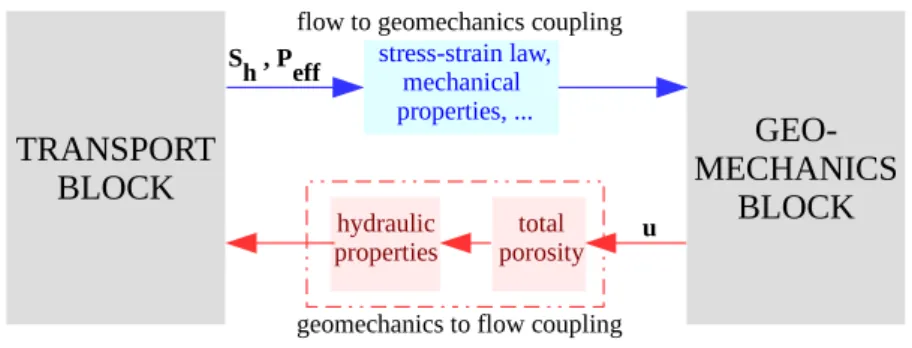
In a typical gas hydrate reservoir, the structure of the sediment is expected to change due to two distinct effects: (1) the changing hydrate saturation, and (2) the sediment deformation. What complicates the matter further is that the hydrate provides additional strength to the sediment through a cementation-like effect, thereby, effectively coupling the two inputs; hydrate saturation, and sediment deformation. For any detailed hydro-geomechanical description of the gas production from gas hydrate-bearing sediments, it is impera- tive to analyze how the transport processes (i.e., flow and chemical processes) would respond to any given geomechanical input. As can be expected, this is a rather challenging task due to the complexity of the interactions. In our model, we simplify the mathematical description of the coupled hydro-geomechanical processes by conceptualizing that the model can be decomposed into two distinct model blocks: transport- block and geomechanics-block, with the coupling between the two manifesting as changes in properties of each model block (see Figure 1). The transport-block solves for the hydrate phase change and the noniso- thermal, two-phase, two-component flow of water and methane gas, while the geomechanics-block solves for the sediment displacements. This decomposition is based on the simplifying assumption that the soil grains constitute the skeleton of the porous matrix, while the gas hydrate enhances the mechanical proper- ties of this skeleton without actively bearing the load. The relative deformation of the gas hydrate phase with respect to the soil skeleton is ignored. This assumption allows us to distinguish between thetotal porosityand theapparent porosity. The total porosity characterizes the total pore volume, i.e., the volume not occupied by the soil grains, while the apparent porosity characterizes the actual pore volume which is available for the fluid flow. The deformation of the hydrate-bearing sediment directly affects only the total porosity. The evolution of the actual or apparent porosity field is then modeled by scaling the total porosity with functions of hydrate saturation through simple geometric arguments. To make the physical meaning clear, the apparent porosity is the actual measured quantity, while the total porosity is a mathematical con- struct which allows us to isolate the effects of sediment deformation from those of hydrate phase change.
We also assume that those properties of the transport-block which depend on the sediment structure (i.e., hydraulic properties like permeability, capillary pressure, specific surface area, tortuosity, etc.) can be mod- eled as amultiplicative decompositionof functions of total porosity and hydrate saturation. In effect, with these simplifications, we can describe all feedback from geomechanics-block to the transport-block through a single transfer variable: total porosity, and this forms a central feature of our coupling concept.
Figure 1.Coupling concept.
In this study, through numerical simulation of a highly controlled high-pressure triaxial experiment com- bined with methane hydrate formation and dissociation, we aim to establish whether this coupling concept is effective in capturing the overall impact of geomechanics on the gas production behavior.
To be able to test the coupling with confidence, there are two important prerequisites: (1) a well-tested model for the transport-block, and (2) a good enough estimation of the displacement field. The validation of the transport-block in our hydrate reservoir model was performed in our earlier study [Gupta et al., 2015].
For the second prerequisite, however, we require a suitable constitutive model for describing the stress- strain response of the hydrate-bearing sediment. A number of nonlinear elastic [e.g.,Yu et al., 2011;Miyazaki et al., 2011a,], elastoplastic [e.g.,Klar et al., 2010;Uchida et al., 2012;Sun et al., 2015;Lin et al., 2015], and elas- toviscoplastic [e.g.Kimoto et al., 2010] constitutive models have been proposed in the recent years to model the geomechanical behavior of gas hydrate-bearing sediments. The stress strain relation in these models is quite complex. Variationally consistent formulations result in nonlinear and nonsmooth inequality settings.
These can be reformulated in terms of nonlinear complementarity functions to which semismooth Newton algorithms as iterative solvers can be applied, which converge locally. To enlarge the local convergence radius, suitable regularization and damping strategies can be designed [Hager and Wohlmuth, 2009, 2010].
Only in special situations existence and uniqueness is given, and often, only local existence is guaranteed and path dependent solutions exist. We refer toMielke[2004, 2009] and the references therein for existence results at finite strain. However, none of these results can be directly applied to our setting since we have a fully coupled hydrate system involving more nonlinearities in the bidirectional couplings. Additionally, the constraints of the system involve inequalities which are nonlinear and nonsmooth, leading to a model with a large number of parameters which often makes model calibration challenging and unreliable. To the best of our knowledge, none of these models have been validated in coupled hydro-geomechanical settings in the context of gas production from gas hydrate reservoirs, and have a large uncertainty associated with their predictive capabilities in highly dynamic conditions. In this study, it is of particular interest to reduce the complexity of the geomechanics-block as much as possible in order to reduce the uncertainty associ- ated with the choice of a constitutive model. We, therefore, chose a uniquely invertible linear-elastic consti- tutive model in the geomechanics-block of our hydrate reservoir model. We account for the stiffening effect due to gas hydrates by parameterizing the Young’s modulus as a function of hydrate saturationSh [Santamarina and Ruppel, 2010]. We also account for material compressibility with respect to hydrostatic pressure. The pressure dependence of compressibility and theShdependence of Lames parameters intro- duces a weak nonlinearity in the geomechanics-block. The numerical implementation of the poroelastic model and the transport-to-geomechanics coupling in our hydrate reservoir model was also validated in our earlier study [Gupta et al., 2015].
In general, poroelasticity is not a realistic model for the geomechanical description of cemented granular materials where the stress-strain response is typically nonlinear, and the shear-volumetric coupling (dilat- ancy) is of particular importance. Therefore, in order to validate our coupling concept within the constraints stated above, we control our triaxial experiment very carefully in a way that ensures that the assumptions of poroelasticity remain valid throughout the periods of interest for numerical simulation.
2. Hydrate Reservoir Model
2.1. Mathematical Model
Our model considers kinetic hydrate phase change and nonisothermal, multiphase, multicomponent fluid flow through poroelastic porous medium. The model assumes that the porous medium is composed of threecomponents:CH4,H2O, and methane hydrate (CH4NhH2O), which are present in three distinctphases:
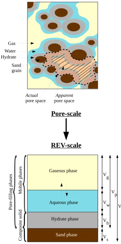
gaseous, aqueous, and solid. The gaseous phase comprises of methane gas and water vapor. The aqueous phase comprises of water and dissolved methane. The solid phase comprises of pure methane hydrate and sand grains. The sand grains are assumed to form a material continuum which provides the skeletal struc- ture to the porous medium. We shall refer to this assolid matrix. The aqueous, gaseous, and hydrate phases exist in the void spaces of this solid matrix (see Figure 2).
We assume that the hydrate cements the sand grains in the mechanical sense (i.e., without forming any chemical bonds), such that the sand and hydrate together form acomposite solid matrix. The relative defor- mation of the gas hydrate phase with respect to the soil skeleton is ignored. This assumption allows us to
write a single momentum balance equation for the composite solid phase, instead of separate ones for the sand and the hydrate phases each. To describe the mechanical behavior of the composite solid matrix, we make a further simplifying assumption that the sand grains form the primary load-bearing structure, while the hydrates enhance the mechanical strength and stiffness of this structure without bearing any load themselves. This assumption is also adopted even after hydrate-bearing soil is loaded during depressuriza- tion. Because of this, the constitutive law does not consider stress-relaxation term that accounts for the release of load that has been carried by hydrates as introduced by others [Klar et al., 2010;Uchida et al., 2012].
Figure 2.Pore-scale to REV-scale.
We decompose the mathematical model into transport and geomechanics blocks, and isolate the effects of hydrate phase change and ground deformation through the introduction of the variabletotal porosity. This is justified based on the above assumption that the soil grains constitute the primary load-bearing skeleton of the porous matrix, such that deformation of the hydrate-bearing sediment directly affects only the total porosity. This assumption allows us to solve for the mass balance of soil and hydrates separately, thus con- veniently separating hydrate phase change kinetics from sediment deformation. If, for example, we do not make this assumption, then we would have to solve for the mass balance of soil and hydrate as a single composite phase leading to a strong coupling between hydrate phase change and geomechanics. The model decomposition would not be straightforward in this case, and the evolution of porosity field would be very complex, making the description of the fluid flow and the evolution of the hydraulic properties also significantly more challenging. One clear advantage of this simplification is that it gives a very modular structure to the model, with each model-block operating independently, and communicating with each other through coupling relationships which are neatly resolved with respect to the independent output var- iables of each model-block (see Figure 1). Another important advantage is that the model decomposition allows us to use multirate time-stepping schemes, as discussed inGupta et al. [2016], which can significantly speed up the calculation, especially for 3-D problems.
The mathematical model is described in detail inGupta et al. [2015]. A summary of the governing equations and the constitutive relationships are given in Table 1. The phases occupying the pore space (gaseous, aqueous, hydrate) are denoted by ‘‘b’’5g;w;hrespectively, the mobile phases (gaseous and aqueous) are denoted by ‘‘a’’5g;w, and the mobile molecular components are denoted by ‘‘j’’5CH4;H2O. The solid matrix is designated with the subscript ‘‘s.’’ The sand1hydrate composite solid matrix is designated with the subscript ‘‘sh.’’ ‘‘c’’is used to denote all phases, i.e.,c5g;w;h;ands.
2.2. Primary Variables
The mathematical model consists of the following six governing equations: the mass balance equations (1)–
(4), the momentum balance equation (7) for the composite-solid, and the energy balance equation (8). The momentum balance equations (5) and (6) for the mobile phasesa5g;wgive thea-phase velocities directly, and are thus absorbed in the mass and energy balance equations. We chose the following set of variables as the primary variables: the gas phase pressurePg, the aqueous phase saturationSw, the hydrate phase sat- urationSh, the temperatureT, the total-porosity/, and, the composite-matrix displacementu. All other vari- ables can be derived (explicitly or implicitly) from this set of variables using the closure and constitutive relationships.
2.3. Solution Strategy
We use an iteratively coupled solution strategy. The mathematical model is decomposed into three parts:
1. transport-block (Ff), comprised of the mass balance equations forCH4,H2O, and Hydrate, and the energy balance equation,
2. geomechanical-block (Fg), comprised of the momentum balance equation for composite solid phase, and
3. porosity-equation (F/), comprised of the mass balance equation for the sand phase.
Ff is solved for the variablesPg,Sw,Sh, andT,Fgis solved for displacementsu, andF/is solved for total porosity/.Ff andF/ are spatially discretized using a fully upwinded cell-centered finite volume method.
Orthogonal grids aligned with the principal axes are defined and a control-volume formulation with two- point flux approximation (TPFA) is used.Fg is discretized using Galerkin finite element (FEM) method defined onQ1 elements. An implicit Euler time-stepping scheme is used for marching forward in time. The solution for a given time step involves two iterative loops, theinner loopand theouter loop. Theinner loop uses Newton’s method and SuperLU [Demmel et al., 1999] linear solver to solve each ofFf;Fg, andF/, thus taking care of the decoupled solution. Theouter loopreintroduces the coupling between Ff;Fg, and F/ through a block Gauss Seidel iterative scheme.
The numerical scheme is implemented in the C11based DUNE-PDELab framework [Dedner et al., 2012], and is capable of solving problems in 1-D, 2-D, and 3-D domains.
Table 1.Summary of the Mathematical Model
Governing Equations Equation No.
Mass balance for each mobile component j5CH4;H2O
X
a
@t / qavjaSa
1X
a
r / qavjaSava;t
5X
a
r /SaJja
1g_j1X
a
q_jma1S_jext (1),(2)
Mass balance for hydrate phase
@tð/ qhShÞ1r / qhShvh;t
5g_h (3)
Mass balance for sand phase
@t½ð12/Þqs1r ð12/Þqð svsÞ50 (4)
Momentum balance for mobile phases a5g;w
va52Kklra
aðrPa2qagÞ(Darcy’s Law) (5),(6)
Momentum balance for composite-solid
r r1q~ mg50 (7)
where,qmis the bulk density given byqm5X
b
/Sbqb
1ð12/Þqs Energy balance
@t ð12/Þqsus1X
b
/Sbqbub
" # 1X
a
r / qavjaSava;tha
5r keffc rT1Q_h1X
a
q_jmaha
(8)
where,
kceff5ð12/Þkcs1X
a
X
j
/ vjaSakca
1/Shkhc
ha5 ðT
Tref
CpadT uc5
ðT Tref
CvcdT Closure relationships
Relationship between phase pressures
Pg2Pw5PcðSweÞ (9)
Summation relationships
X
b
Sb51 (10)
8a:X
j
vja51 (11),(12)
Constitutive relationships 1. Vapor-liquid equilibrium
Using Henry’s Law and Raoult’s Law for ideal gas-liquid solutions, For dissolved
methane:
vCHw45HðTÞvCHg4Pg
For water vapor:
vHg2O5vHw2OP
sat H2OðTÞ
Pg
where,H(T) is the Henry’s constant for methane dissolved in water calculated using the empirical relation from NIST database [Sander, 2015], andPsatH2Ois saturated water vapor pressure calculated using Antoine’s equation.
2. Diffusive mass-transfer flux
Fick’s law: Jja52sDaqarvja
where,Dais the binary diffusion coefficient.Dgis estimated using the empirical relationship proposed byStattery and Bird[1958] for low density binaryCH42H2Osystem.Dwis estimated using the Wilke-Chang correlation [Himmelblau, 1964] for dilute associated liquid mixtures is used.
3. Hydrate phase change kinetics
Nonequilibrium phase change of methane hydrate is modeled by the Kim-Bishnoi kinetic model [Kim et al., 1987].
Gas generation rate g_CH45kreacMCH4Ars Pe2fg
(13) where,kreacis the rate of kinetic phase-change,Peis the hydrate equilibrium pressure, modeled as [Kamath, 1984],
Pe5A1expA22AT3
, (14)
fgis the gas fugacity calculated using the Peng-Robinson EoS for methane gas, and,Arsis the specific reaction sur- face area modeled asArs5CrAs, where,Asis the total surface area andCris the ratio of the active reaction sur- face to the total surface area.AsandCrare modeled using the correlations proposed byYousif[1991] andSun and Mohanty[2006], respectively.
Water generation rate g_H2O5_gCH4NHydMH2O MCH4
(15) Hydrate consumption
rate
2_gHyd5_gCH4MMHyd
CH4
(16) Heat of hydrate
dissociation
Q_h52_MgHyd
Hyd B12BT2 (17)
4. Properties of the fluid-matrix interaction
Capillary pressure Pc5Pc0fSPchð Þ Sh f/Pcð Þ/ (18)
where,Pc0is capillary pressure for undeformed, unhydrated solid matrix, given by Brooks-Corey relationship,
Pc05PentrySwe21=kBC, (19)
and,fSPchð ÞSh andf/Pcð Þ/ are scaling factors to account for the effects ofSh[Rockhold et al., 2002] and/(Civan’s power law correlationCivan[2000]) respectively,
fSPch5ð12ShÞ2
3kBC21
3kBC and,f/Pc5//0 12/12/
0
2 (20)
Intrinsic permeability K5K0fSKhð Þ Sh f/Kð Þ/ (21)
3. Material and Methods
We performed a controlled triaxial volumetric strain test on a sand sample in which methane hydrate was first formed under controlled effective stress and then dissociated via depressurization under controlled total stress. Gas hydrate in our experiment was initially formed by pressurizing partially water-saturated sand with gaseous methane to reach a gas hydrate saturation of 0.4, and remaining methane gas was replaced with seawater before the sample was depressurized stepwise. Confining and axial loads in the tri- axial testing were applied isotropically and were carefully controlled to keep the deformation of the sample small and well within the assumptions of poroelasticity.
3.1. Experimental Setup and Components
Experiments were carried out in the custom-made high-pressure apparatus NESSI (Natural Environment Simulator for Subseafloor Interactions) [Deusner et al., 2012], which is equipped with a triaxial cell mounted in a 40 L stainless steel vessel (APS GmbH Wille Geotechnik, Rosdorf, Germany). The sample sleeve is made from FKM, other wetted parts of the setup are made of stainless steel. Salt water medium was stored in reservoir bottles (DURAN, Wertheim, Germany) prior to use in experiments, and the seawa- ter medium was pressurized in an additional pressure vessel (Parr Instrument GmbH, Frankfurt, Ger- many) to allow fast transfer into the sample vessel. Fluid pressure in the sample vessel was adjusted with a back-pressure regulator valve (TESCOM Europe, Selmsdorf, Germany). Experiments were carried out in upflow mode with injection ofCH4gas and seawater medium at the bottom of the sample prior to and after gas hydrate formation (Figure 3a), respectively, and fluid discharge at the top of the sample during depressurization (Figure 3b). Axial and confining stresses, and the sample volume changes were moni- tored throughout the experimental period. Axial and confining stresses were controlled using high- precision hydraulic pumps and actuators (VPC 400, APS GmbH Wille Geotechnik, Rosdorf, Germany), and changes in hydraulic fluid volumes were converted to calculate sample volume changes. Pore pressure was measured in the influent and the effluent fluid streams close to the sample top and bottom. The experiment was carried out under constant temperature conditions. Temperature control was achieved with a thermostat system (T1200, Lauda, Lauda-K€onigshofen, Germany). Produced gas mass flow was analyzed with mass flow controllers (EL FLOW, Bronkhorst, Kamen, Germany). For control purposes, bulk effluent fluids were also collected inside 100 L gas tight TEDLAR sampling bags (CEL Scientific, Santa Fe Springs CA, USA). The sampling bags were mounted inside water filled containers. After expansion of the effluent fluids at atmospheric pressure, the overall volume was measured as volume of water displaced from these containers.
Table 1.(continued)
Governing Equations Equation No.
where,K0is intrinsic permeability of the undeformed, unhydrated solid matrix, and,fSKhð ÞSh andf/Kð Þ/ are scaling factors to account for the effects ofSh[Rockhold et al., 2002] and/[Civan, 2000] respectively,
fSKh5ð12ShÞ196and,f/K5//
0 f/Pc 22 (22)
Relative permeabilities
Relative permeabilities of the mobile phases are modeled using Brooks-Corey model in conjunction with the Burdine theorem [Burdine, 1953], as
krw5S
213kBC kBC
we and,krg5ð12SweÞ2 12S
21kBC kBC we
where,Swe512SSw
h
(23)
Hydraulic tortuosity s5/nwhere, 1n3 (24)
5. Poro-elasticity Effective stress
principle
Effective stress concept introduced byTerzaghi[1925] and modified byBiot[1941] is used.
r5~~ r01abiot SgPg1SwPw Sg1Sw
~I (25)
where,r~is the total stress acting on the bulk porous medium, andr~0is the effective stress acting on the composite skeleton.
abiotis the Biot-Willis constant [Biot and Willis, 1957].
Linear elastic law r~052Gsh~1kshðtr~Þ~I (26)
where,~is the linearized strain, given by~512ðru1rTuÞ (27)
and,Gshandkshare the Lame’s parameters.
Young’s modulus Young’s modulusEshis modeled using the parameterization proposed bySantamarina and Ruppel[2010]:
Esh5Es1SchEh
where,EsandEhare the Young’s modulus of hydrate-free sand and hydrate, respectively. (28)
3.2. Sample Preparation and Mounting
The sediment sample was prepared from quartz sand (initial sample porosity: 0.35, grain size: 0:120:6 mm, G20TEAS, Schlingmeier, Schw€ulper, Germany), which was mixed with deionized water to achieve a final water saturation of 0.4 relative to the initial sample porosity. The partially water-saturated and thoroughly
a) Gas hydrate formation
b) Depressurization and gas production
Figure 3.Simplified flow schemes for relevant period. (a) Gas hydrate formation. (b) Depressurization and gas production.
homogenized sediment was filled into the triaxial sample cell to obtain final sample dimensions of 360 mm in height and 80 mm in diameter. The sample geometry was assured using a sample forming device. The sample was cooled to 28C after the triaxial cell was mounted inside the pressure vessel. Initial water permeability of the gas hydrate-free sediment was esti- mated to be 5310210m2.
3.3. Experimental Procedure 3.3.1. Gas Hydrate Formation
Prior to the gas hydrate formation, the partially water-saturated sediment sam- ple was isotropically consolidated to 1 MPa effective stress under drained conditions. It should be noted that the apparent effective stress is monitored and controlled as differential pressure between the confining hydraulic fluid pressure of the reactor and the gas pressure in the sample pore space. Measurements and control algorithms do not take into account the changes in effective stress due to changes in water saturation and capillary pressure. Thus, only the apparent effective stress is directly accessible from experimental procedures. The sample was flushed withCH4 gas to replace air with methane. The sample was, subsequently, pressurized withCH4 gas to approximately 12.5 MPa (Figure 3a). During pressurization withCH4 gas and throughout the overall gas hydrate for- mation period, formation stress condition of 1 MPa effective stress were maintained using an auto- mated control algorithm. The formation process was continuously monitored by logging theCH4 gas pressure. Mass balances and volume saturations were calculated based on CH4 gas pressure and initial mass and volume values. Gas hydrate formation was terminated after 1.84 mol ofCH4-hydrate had been formed after approximately 6 days, corresponding to CH4-hydrate saturation of 0.39. The sample was cooled to258C and stress control was switched to constant total isotropic stress control at approximately 9 MPa before the sample pore space was depressurized to atmospheric pressure and the remainingCH4
gas in the pore space was released. System repressurization and water saturation of the pore space was achieved by instant filling and repressurization with pre-cooled218C saltwater medium according to the seawater composition. Hydrate dissociation during the brief period of depressurization was minimized by taking advantage of the anomalous self-preservation effect, which reaches an optimum close to the cho- sen temperature [Stern et al., 2003]. After completion of the gas-water fluid exchange, the sample temper- ature was readjusted to 28C.
3.3.2. Depressurization and Gas Production
The sample pore space was depressurized and gas produced by stepwise decrease of back pressure at con- stant isotropic total stress (Figure 3b). Overall fluid production (water andCH4gas) was monitored after depressurization at atmospheric pressure after temperature equilibration.
4. Numerical Simulation
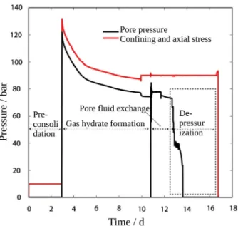
The overall experiment was carried out in four steps, viz., (1)preconsolidation, (2)gas hydrate formation, (3) pore-fluid exchange, and (4)depressurization, as described in section 3. During steps 1 and 2, the sample was maintained under a defined effective loading with the confining and the axial stresses were controlled to remain 10 bar above the pore pressure. During steps 3 and 4, the total isotropic stress was controlled to remain at a constant level (see Figure 4). The experiment was performed over a total period of about 16.8 days. Theperiods of interest for this simulation are: (1) fromDay– 3 toDay– 10, corresponding to gas hydrate formation, and (2) fromDay-12:8 toDay-13:8, corresponding to depressurization and gas produc- tion. We simulate both of these periods separately.
Figure 4.Overview of themeasuredpressure and stresses over time.
4.1. Computational Domain
Assuming that the sand sample is axially symmetric, a 2-D radial plane of dimensions 360 mm340 mm is chosen as the computational domain. The dimensions correspond to the physical size of the sample. The domain is discretized into 7238 cells.
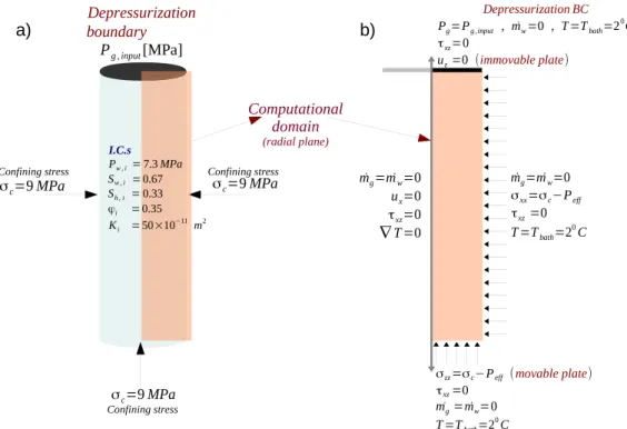
4.2. Test-setting
4.2.1. Gas Hydrate Formation Period
The schematic of the hydrate formation test is shown in Figure 5. The schematic also shows the initial and boundary conditions. The simulation is run untiltend5604,800 s (i.e., 7 days) using a maximum time step size of 120 s.
4.2.2. Depressurization and Gas Production Period
The schematic of the depressurization test is shown in Figure 6. The schematic also shows the initial and boundary conditions. The simulation is run untiltend586,400 s (i.e., 1 day) using a maximum time step size of 120 s.
4.3. Properties and Parameters
The material properties and model parameters chosen for this simulation are listed in Table 2. The values of the thermal conductivities, specific heat capacities, dynamic viscosities, and densities for each phase are chosen from standard literature, the references to which are included in the table. The Brooks-Corey param- eters are chosen from the range of typically expected values for sand samples.
Table 2.Material Properties and Model Parameters
Thermal Conductivities Ref.
kcg 20:8863102210:24231023T20:69931026T210:12231028T3 Wm21K21 Roder[1985]
kcw 0:3834 lnðTÞ21:581 Wm21K21 Wagner and Kretzschmar[2008]
kch 2.1 Wm21K21 Sloan and Koh[2007]
kcs 1.9 Wm21K21 Esmaeilzadeh et al. [2008]
Specific heat capacities
Cpg DCpresgð123813:13T17:931024T2 26:8631027T3Þ
Jkg21K21 Peng and Robinson[1976];
Esmaeilzadeh et al. [2008]
Cvg Cpg1RCH4 Jkg21K21
Cpw 4186 Jkg21K21 Wagner and Kretzschmar[2008]
Cvw Cpw1RH2O Jkg21K21
Cvh 2700 Jkg21K21 Sloan and Koh[2007]
Cvs 800 Jkg21K21 Esmaeilzadeh et al. [2008]
Dynamic viscosities
lg 10:431026 273:151162
T1162
T
273:15
1:5 Pas Friend et al. [1989]
lw 0:001792 exp½21:9424:80273:15T
16:74273:15T 2
Pas Wagner and Kretzschmar[2008]
Densities
qg Pg
zRgT kgm23 Peng and Robinson[1976]
qw vapor: 0:0022PTg kgm23 Wagner and Kretzschmar[2008]
liquid: 1000 kgm23 Wagner and Kretzschmar[2008]
qh 900 kgm23 Sloan and Koh[2007]
qs 2100 kgm23
Hydraulic properties
kBC 1.2 Helmig[2016]
Pentry 50 kPa Helmig[2016]
Hydrate kinetics
kreac Formation: 0:2310211 molm22
Dissociation: 3:2310210 Pa21s21
NHyd 5.75
Pe;0 A15106;A2538:98;A358533:8 Pa Kamath and Holder[1987]
Q_h B1556599;B2516:744 Wm23 Esmaeilzadeh et al. [2008]
Poroelasticity parameters
abiot 0.8 Verruijt[2008]
msh 0.15 Miyazaki et al. [2011b]
Formation dissociation
Es 32 160 MPa
Eh 250 360 MPa
c 1 3
The most important properties and parameters relevant to the simulation of the experimental data arise from (1) the hydrate-phase-change kinetics, and (2) the poroelastic behavior of the hydrate-bearing sediments.
Figure 5.Test setting for thegas hydrate formationperiod. (a) The sample and the initial conditions, and (b) the 2-D computational domain and the boundary conditions.
Figure 6.Test setting for thedepressurization and gas productionperiod. (a) The sample and the initial conditions, and (b) the 2-D com- putational domain and the boundary conditions.
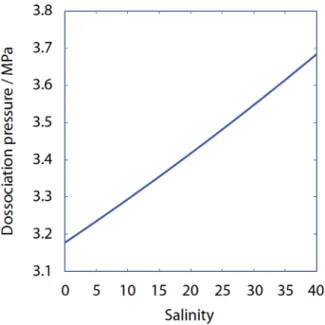
The hydrate phase-change is modeled by equations (13), (15)–(17). The hydrate- phase equilibrium pressurePein equation (13) is modeled in accordance with the findings ofKamath[1984]. For hydrates in pure water, the equilibrium pressure depends only on the temperature. How- ever, for hydrates in sea water (which is the case for our sample), the equilibrium pressure also depends on the salinity, as shown in Figure 7. We account for the effect of salinity on the hydrate equilib- rium pressure through linear curve fitting on dissociation pressure versus salinity curve.
The reaction surface area,Ars, in equation (13), describes the surface area available for the kinetic-reaction, and puts a limit on the mass transfer during hydrate for- mation and dissociation. As the hydrate saturation in the pore-space increases, the availability of free surface for hydrate formation to occur decreases, and vice versa. Additionally, for hydrate formation, availability of both gas and water in sufficient quantities in the pore-space is a necessary condi- tion. This behavior ofArsis modeled using the parameterization proposed bySun and Mohanty[2006].
The rate of reaction,kreac, is a free parameter in our simulation which is used to calibrate the hydrate- kinetics model with respect to the experimental data. In the table we can see that the values ofkreac, for both hydrate formation as well as dissociation periods, lie well within the range reported in the literature.
The poroelastic behavior of the hydrate-bearing sediment is characterized by three parameters, viz.,Biot’s constantabiot, Poisson ratiomsh, and Young’s modulusEsh. Biot’s constant is chosen from a range of typically expected values. The Poisson’s ratio is assumed to be a constant independent of the hydrate saturation fol- lowing the experimental studies byMiyazaki et al. [2011b];Lee et al. [2010a]. The Young’s modulus is mod- eled using the parameterization proposed bySantamarina and Ruppel[2010], given by equation (28). The Young’s modulusEshis afree parameterwhich is used to calibrate the poroelasticity model with respect to the experimental data.
4.4. Simulation Results
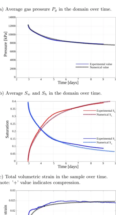
As discussed above, we essentially choseonefree parameter in kinetics, i.e.,kreac, andonefree parameter in linear-elasticity, which isEsh, to calibrate the kinetic and the mechanical models separately. With these cali- brated models, we simulate numerically the coupled (thermo-chemo)-hydro-geomechanical response of the sand sample in triaxial test-setting using our gas hydrate reservoir model. The numerical results, together with the corresponding experimental data, are plotted in Figure 9 for the gas hydrate formation period, and in Figure 8 for the hydrate dissociation period.
In thegas hydrate formation period, methane gas in the free pore space is continuously consumed and average bulk gas pressure is decreased (see Figure 9a). Clearly, the rate of gas hydrate formation is not con- stant. In the beginning, after the sample is pressurized at constant isotropic effective stress, gas hydrate for- mation from free methane gas and pore water is fast, but the rate of formation steadily decreases due to mass transfer limitations and shrinking reaction surfaces. In accordance to that, after pressurization the gas hydrate saturation increases rapidly and the water saturation decreases proportionally (Figure 9b). Note that the reported values of phase saturations are calculated based on initial values and gas pressure meas- urements. The volumetric strain shows a fast positive response during early gas hydrate formation at rela- tively low gas hydrate saturations, and sample stiffness increases at higher gas hydrate saturations (Figure 9c).
The fast volumetric strain response that occurs at constant apparent effective stress results from changes in
Figure 7.Effect of salinity on hydrate stability curve (atTbath528C).
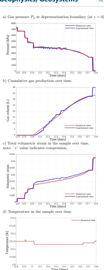
Figure 8.Comparison of the simulation results with the experimental results for thedepressurization and gas productionperiod.
(a) Gas pressurePgat depressurization boundary (atz50). (b) Cumulative gas production over time. (c) Total volumetric strain in the sample over time. Note: ‘‘1’’ value indicates compression. (d) Temperature in the sample over time.
water saturation and, thus, capillary pressure, which is not monitored experimentally, but considered in the numerical simulation.
During thegas hydrate dissociation period, pressure is decreased step-wise until methane hydrates become unstable at the respective P-/T-conditions. Figure 8a shows the numerically computed gas phase pressure in the
Figure 9.Comparison of the simulation results with the experimental results for thegas hydrate formationperiod. (a) Average gas pres- surePgin the domain over time. (b) AverageSwandShin the domain over time. (c) Total volumetric strain in the sample over time. Note:
‘‘1’’ value indicates compression.
sample. The gas production is plotted in Figure 8b. With the onset of gas hydrate dissociation after reaching the hydrate stability boundary, pressure is maintained at a relatively constant level because hydrate dissociation and gas production equilibrate dependent on experimental and technical conditions.
Volumetric strain during gas hydrate dissociation, plotted in Figure 8c, is dependent on effective stress and gas hydrate saturation through the sample stiffness, which decreases with the ongoing gas hydrate dissociation and gas production.
Figure 8d shows the numerically computed temperature profile of the sample during dissociation. The model predicts that subcooling from gas hydrate dissociation is quite small, which is expected since the experiment was performed under isothermal temperature control.
5. Discussion and Outlook
In our combined experimental-numerical study, we consider dynamic gas hydrate formation and dissociation in sandy sediment under isotropic compressive loading and show that a simplified coupling concept is capa- ble of reproducing the essential bulk physical behavior, including volumetric strain and gas production.
The assumption that the soil is the primary load-bearing constituent is central to our model concept. This assumption is most reasonable for the pore-filling hydrates with low saturations where the hydrates form by nucleating on sediment grain boundaries and grow freely into pore spaces without entering the pore- throats. For hydrates formed in partially water saturated sands, as is the case in our experiment, it is well known that the hydrates nucleate preferentially in the pore-throats and contribute to the sediment stiffness already at low gas hydrate saturations. For hydrate saturations between 0:25 and 0:4, the hydrates are expected to transition toward a load-bearing habit [Waite et al., 2009]. In our experiment, we obtain a maxi- mum hydrate saturation of0:4. Our numerical results suggest that inwell-consolidatedsands, our assumption of soil forming the primary load-bearing skeleton remains valid even for hydrate saturations which lie in the transition zone between pore-filling and load-bearing habits. We hypothesize that this is because inwell-consol- idatedsands, the deformation of hydrates relative to the soil skeleton is quite small in the transition zone. How- ever, for higher hydrate saturations where hydrates become fully load-bearing, we expect strong limitations to this coupling concept. Furthermore, for massive hydrates with saturations exceeding 0.8, we even expect that the hydrate and the soil phases can no longer be modeled as a single composite phase, and new model con- cepts are necessary to consistently describe the interface conditions between the hydrate and the soil phase boundaries.
Our experiment was focused on analyzing deformation under variable gas hydrate saturation, and a wide range of effective stress loading, controlled between 1 and 9 MPa. To limit the bulk sample deformation and relative grain-to-grain movement only isotropic stresses were applied. Gas hydrates were formed after isotropic consolidation to 1 MPa using the excess-gas-method [Chong et al., 2016;Choi et al., 2014;Jin et al., 2012;Priest et al., 2009]. After gas hydrate formation, the remaining gas was fully replaced with seawater.
After gas-seawater replacement, the sample was equilibrated for approximately 5 days to allow for gas hydrate alteration before the sample was depressurized. A poroelasticity framework was chosen for describ- ing the mechanical behavior of the sediment in order to minimize the uncertainties arising from unknown mechanical behavior of gas hydrate-bearing sediments. The deliberate choice of a simple constitutive law with a limited number of parameters, in contrast to using more complex elastoplastic modeling approaches, is justified by the design of the experimental test case. It is important to note that, within the constraints of small-strain deformations and pore-filling hydrates, the coupling concept presented here does not depend on the stress-strain constitutive law as such. The concept of poroelasticity is, therefore, sufficient to test the validity of our coupling concept provided that the design of the experiment ensures that the sample defor- mations remain small and well within elastic limit. For large deformations, the coupling concept is not vali- dated so far.
To approximate our experimental data, we treated the kinetic termkreacin the transport block as a fitting parameter. Similarly, we used fitting of the stiffness model parameters to match the experimental volumet- ric strain behavior. We chose a functional dependence of composite modulusEshon hydrate saturationSh
as proposed bySantamarina and Ruppel[2010] and other authors [Rutqvist et al., 2009;Klar et al., 2010, 2013]. Knowledge about mechanical stiffness and strength properties of gas hydrate-bearing sediments is
still limited. Experimental analysis of mechanical properties is problematic, because it is equally important to control effective stress conditions and phase saturations, and there are no test procedures available to guarantee homogeneous gas hydrate saturations and full water saturation. Further, mechanical properties are strongly dependent on gas hydrate-sediment fabrics and formation procedures, and effects from dynamic changes in gas hydrate saturation, distributions, and alterations of gas hydrate-sediment fabrics needs further investigation and development of novel test procedures [Deusner et al., 2016] particularly for dynamic test scenarios. Overall, the calibrated values forEshfrom our study are in accordance with earlier experimental and numerical studies, which reported Young’s modulus or secant stiffness in a wide range of approximately 100–400 MPa for relevant gas hydrate concentrations [Brugada et al., 2010;Miyazaki et al., 2010;Lee et al., 2010b;Yun et al., 2007]. Although the composite modulusEshwas treated as a free fitting parameter and initialized based on apparent stress-strain behavior during the intervals of known and con- stant gas hydrate saturations, physically meaningful values for individual moduliiEsandEhwere obtained.
Esfor the sediment without gas hydrate reflected stiffness behavior typical for loose soil during gas hydrate formation while the sample was normally consolidated at low effective stress. The results from the numeri- cal simulation suggest that an apparent step-like increase in bulk composite stiffness (i.e., the change of apparentEsh from 132 to 183 MPa) occurred during the time interval between the completion of gas hydrate formation and the start of depressurization. We assume that this response was caused by the high transient effective stress and the composite sediment consolidation, which could not be avoided during the gas-water exchange. In order to accomplish the replacement of gas with water sufficiently fast, and to mini- mize gas hydrate dissociation during the short time interval of gas-water exchange, the confining stress instead of the apparent effective stress was controlled at a constant value during gas-water exchange. In fit- ting the model to the experimental data, we adjusted bothEsandEhrather than constraining the effect of consolidation to one of the parameters a priori. However, the validity of this assumption needs to be further investigated using advanced geotechnical and microstructural analyses. Furthermore, it needs to be consid- ered that the poroelasticity model adopted for testing our coupled numerical simulation scheme does not explicitly consider effective stress-dependent changes in the moduliiEsandEh, which could also contribute to the apparent differences inEshduring gas hydrate formation and dissociation periods. In our simulation, the composite modulusEshdepends almost linearly onShduring gas hydrate formation, while during the hydrate dissociation period the dependence ofEshonShis smaller. Figure 10 shows the volumetric-strain plotted over time for the depressurization period for different functional dependences ofEshonSh (i.e., c50:5;1;2;3;5). Our simulation results indicate that an exponent c53 is a reasonable approximation.
Santamarina and Ruppel[2010] suggest thatShtends to be raised to a power larger than 1, which reduces the impact on stiffness at low gas hydrate saturations relative to that for high gas hydrate saturations. Since gas hydrates formed using the excess-gas-method are predominantly located in the pore throats rather than in the free pore space, the linear and relatively stronger dependence ofEshonShduring formation appears reasonable. The weaker dependence ofEshon gas hydrate saturation during dissociation is also
Figure 10.Volumetric strain curves for different functional dependences ofEshonSh(i.e.,c51;2;3;5) for thedepressurization and gas productionperiod. Note: ‘‘1’’ value indicates compression.