RESEARCH ARTICLE
10.1002/2017GC006995
Assessing marine gas emission activity and contribution to the atmospheric methane inventory: A multidisciplinary approach from the Dutch Dogger Bank seep area (North Sea)
M. R€omer1 , S. Wenau1 , S. Mau1 , M. Veloso2, J. Greinert2 , M. Schl€uter3, and G. Bohrmann1
1Department of Geosciences, MARUM—Center for Marine Environmental Sciences, University of Bremen, Bremen, Germany,2GEOMAR Helmholtz Centre for Ocean Research Kiel, Kiel, Germany,3Alfred Wegener Institute, Helmholtz Centre for Polar and Marine Research, Bremerhaven, Germany
Abstract
We present a comprehensive study showing new results from a shallow gas seep area in 40 m water depth located in the North Sea, Netherlands sector B13 that we call ‘‘Dutch Dogger Bank seep area.’’ It has been postulated that methane presumably originating from a gas reservoir in600 m depth below the seafloor is naturally leaking to the seafloor. Our ship-based subbottom echosounder data indicate that the migrating gas is trapped in numerous gas pockets in the shallow sediments. The gas pockets are located at the boundary between the top of the Late Pliocene section and overlying fine-grained sediments, which were deposited during the early Holocene marine transgression after the last glaciation. We mapped gas emissions during three R/V Heincke cruises in 2014, 2015, and 2016 and repeatedly observed up to 850 flares in the study area. Most of them (80%) were concentrated at five flare clusters. Our repeated analysis revealed spatial similarities of seep clusters, but also heterogeneities in emission intensities. A firstcalculation of the methane released from these clusters into the water column revealed a flow rate of 277 L/min (SD5140), with two clusters emitting 132 and 142 L/min representing the most significant seepage sites. Above these two flare clusters, elevated methane concentrations were recorded in atmospheric measurements. Our results illustrate the effective transport of methane via gas bubbles through a40 m water column, and furthermore provide an estimate of the emission rate needed to allow for a contribution to the atmospheric methane concentration.
1. Introduction
The application of advanced hydroacoustic techniques reveals that natural marine methane seepage to the hydrosphere is occurring along almost all continental margins. Methane can migrate through the sediments and enter the water column either dissolved within pore water or, in case of over- saturation, as free gas phase (bubbles). While the microbial filter of the shallow seabed efficiently lowers the release of dissolved methane to the water column [e.g.,Sommer et al., 2006], gas bubbles bypass this filter. When released into the water column and rising to the sea surface, methane gas bubbles are affected by dissolution due to the concentration gradient between the bubble and under-saturated ocean water as well as gas stripping (N2, O2) from the water into the bubble [e.g.,Leifer and Patro, 2002;
McGinnis et al., 2006;Rehder et al., 2009]. The dissolved methane can be oxidized by microbes and con- verted to CO2[Mau et al., 2015;Reeburgh, 2007;Valentine et al., 2001]. How much methane remains in the bubble depends on the depth of the seep site. Seep sites on shallow continental shelf areas are expected to transport some fraction of the released methane through the water column to the sea surface, where the bubbles burst and directly contribute to the atmospheric methane inventory [Leifer and Patro, 2002]. For dis- solved phase methane, the gas exchange with the atmosphere is influenced by the density stratification in the water column that may limit vertical transport of dissolved gas in the lower part of the water column even at shallow sites. For example, at the 70 m deep Tommeliten area in the North Sea, a summer thermo- cline constrains methane transport to the atmosphere and numerical modeling showed that during this season less than 4% of the gas initially released as bubbles at the seafloor reaches the mixed layer [Schneider von Deimling et al., 2011]. However,Borges et al. [2016] report on intense methane emissions
Key Points:
Several hundred flares were mapped occurring mainly in five distinct clusters
Flare clusters are related to subseafloor gas accumulations at a late-Pleistocene surface
Methane anomalies were detected in the atmosphere above the more intensely emitting clusters
Supporting Information:
Supporting Information S1
Figure S1
Figure S2
Figure S3
Table S1
Table S2
Correspondence to:
M. R€omer, mroemer@marum.de
Citation:
R€omer, M., S. Wenau, S. Mau, M. Veloso, J. Greinert, M. Schl€uter, and G. Bohrmann (2017), Assessing marine gas emission activity and contribution to the atmospheric methane inventory: A multidisciplinary approach from the Dutch Dogger Bank seep area (North Sea),Geochem.
Geophys. Geosyst.,18, 2617–2633, doi:10.1002/2017GC006995.
Received 1 MAY 2017 Accepted 5 JUN 2017
Accepted article online 16 JUN 2017 Published online 20 JUL 2017
VC2017. American Geophysical Union.
All Rights Reserved.
Geochemistry, Geophysics, Geosystems
PUBLICATIONS
from the near-shore southern region of the North Sea characterized by the presence of extensive areas with gassy sediments and further conclude that shallow well-mixed continental shelves and seep areas are hot spots of methane emission and probably underestimated in the global context.
Hydroacoustic mapping using single-beam and multibeam echosounder systems (SBES and MBES, respectively) can detect bubble release from the seafloor. SBES data can be used to quantify gas fluxes based on empirical correlations between measured gas fluxes at the seafloor and their hydroacoustic response [Artemov et al., 2007;Jerram et al., 2015;Nikolovska et al., 2008;Ostrovsky et al., 2008;Muyakshin and Sauter, 2010;Veloso et al., 2015]. More traditionally, the amount of naturally emanating gas entering the hydrosphere was quantified by visually observing bubble flow rates (volume/time) at distinct seep locations and extrapolation to all observed flares. With this approach and an estimate of the seepage area, gas fluxes were derived in the Black Sea [Grei- nert et al., 2010;R€omer et al., 2012a;Sahling et al., 2009], the Makran continental margin [R€omer et al., 2012b], the Cascadia margin at Hydrate Ridge [Torres et al., 2002], the Håkon Mosby mud volcano [Sauter et al., 2006], on the northern US Atlantic margin [Skarke et al., 2014], and also in the North Sea [e.g.,Judd, 2004;Schneider von Deimling et al., 2011]. Derived methane flow rates vary widely between 1.2 and 29,200 ton per year (t/yr) for individual seep sites and can be much larger for entire shelf areas as estimated for the East Siberian Arctic Shelf, which is presumed to be related to thawing submarine permafrost [Shakhova et al., 2014].
Many studies that report gaseous methane output cannot consider spatial and temporal variability, as observations and measurements were usually only done during short time periods of research cruises. But natural gas emissions have often been observed to be highly variable on various time scales [Boles et al., 2001;Greinert, 2008;Kannberg et al., 2013;Schneider von Deimling et al., 2010;Tryon et al., 1999]. In this study, we performed extensive contemporaneous as well as iterative investigations at the North Sea ‘‘Dutch Dogger Bank seep area’’ (Figure 1) focusing on (a) monitoring the activity of gas bubble emission into the water column in three consecutive years, (b) subseafloor mapping to identify gas pockets and pathways that explain spatial variability, and (c) the contribution of released methane to the atmospheric inventory
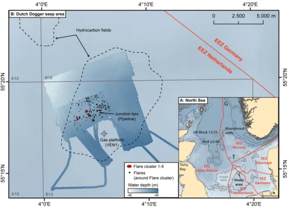
Figure 1.(a) Overview map of the North Sea including locations of the main seep areas and the study area located at the eastern edge of the Dogger Bank in the Netherlands EEZ. G, Gullfaks and T, Tommeliten. (b) Hundreds of flares were detected in the Dutch Dogger Bank seep area, close to a gas platform. The area was mapped during three cruises in 2014, 2015, and 2016 resulting in a bathymetric coverage of about 70 km2.
above bubble emission areas. Our data provide a detailed description of a spatially heterogeneous seep area with flare clusters of different and varying gas emission intensities, which are related to a complex sub- surface structures trapping upward migrating gas. Additionally, our data allow evaluating the contribution of the seep area to methane export into the atmospheric inventory and a comparison of the Dutch Dogger Bank seep area emissions to other known methane seep sites.
1.1. Study Site
The ‘‘Dutch Dogger Bank seep area’’ is located in the central North Sea within the Netherlands sector B13 in about 43 m water depth (Figures 1a and 1b). Toward the north and northwest lies the Dogger Bank, a moraine of Pleistocene age covered by Holocene sand deposits that has been subaerial and connected to the mainland until the end of the last ice age. The seafloor in the study area is flat and lacking morphologi- cal expressions that might be indicative for gas seepage [Schroot et al., 2005]. Nevertheless, seismic and high-frequency acoustic surveys described bySchroot and Sch€uttenhelm[2003] revealed indications of gas in shallow sediments.Schroot et al. [2005] further measured elevated methane concentrations in sediments above zones of acoustic blanking (blocks B13, F3, and F6) and within a pockmark structure (block A11) in the northern part of the Netherlands sector, but occurrences of emanating gas bubbles were only reported for block B13.
In the northern part of the Netherlands North Sea sector, abundant examples of bright spots in seismic records can be seen in the Upper Pliocene-Pleistocene sequences, usually corresponding to low-relief struc- tural highs above salt structures. This area of the North Sea is influenced by the Central Graben which origi- nates from extensional tectonics in the Late Jurassic to Early Cretaceous, leading to defined horst-and- graben structures [Wride, 1995]. Hydrocarbon migration and accumulation are generally related to salt dia- pirism (mainly mobilization of Permian Zechstein evaporites), and associated faulting and gas-charged sand-filled ice-scours and channels are additional gas traps [Schroot and Sch€uttenhelm, 2003;Schroot et al., 2005]. A group of relatively shallow (600–700 m) gas accumulations in blocks A and B, including the one detected in B13 (dashed outline in Figure 1), are large enough to be of economic interest. At B13, gas is pro- duced since December 2011, and the unmanned platform is located about 3 km south of the known gas emission site (Figure 1). Analyses ofd13C CH4from sediment cores at B13 vary between289&and255&
PDB, pointing to a predominantly biogenic origin; however, there are also indications for the presence of higher molecular-weight hydrocarbons [Schroot et al., 2005].
The subseafloor geology of the northern Dutch North Sea sector has evolved from an open marine setting in the Miocene to shallow marine and fluvial settings in the Pleistocene [Kuhlmann and Wong, 2008;Stuart and Huuse, 2012]. The early Pleistocene is characterized by the accumulation of large volumes of sediments in a delta system related to the Baltic River System, producing clinoform sequences that prograde from East to West through the study area [Overeem et al., 2001;Kuhlmann and Wong, 2008;Stuart and Huuse, 2012].
Since the middle Pleistocene the area has been dominated by the rapid changes of warm and cold periods and associated glaciations. In the course of these climate and sea level variations, several sequences of glacial-interglacial sediments have been deposited. These deposits are characterized by an abundance of subglacial tunnel valleys that formed beneath ice sheets and river systems, both related to melt water flows [Huuse and Lykke-Andersen, 2000;Fitch et al., 2005; Kuhlmann and Wong, 2008;Stuart and Huuse, 2012;
Hughes et al., 2016].
2. Methods
2.1. Hydroacoustic Data
Three research cruises have been conducted in the study area with R/V HEINCKE: (1) HE-413 in January 2014, (2) HE-444 in May 2015, and (3) HE-459 in March–April 2016. Intensive mapping with hydroacoustic echosounders was conducted during all of the cruises. The ship speed was typically 5 knots during map- ping, but was decreased to 3 knots for high-resolution surveys of distinct small areas when weather condi- tions allowed for stable surveying of the vessel at such a low speed.
R/V HEINCKE is equipped with a multibeam echosounder (MBES) Kongsberg EM710, a single-beam echosounder (SBES) Simrad EK60, and a subbottom profiler (SBP) Innomar SES-2000 medium, which were all used during the three cruises. Depending on the survey objectives, the echosounders recorded
simultaneously or individually in order to avoid acoustic interferences. The MBES operates at a frequency of 70–100 kHz. A large coverage for bathymetric and seafloor backscatter mapping but also the detec- tion of high backscatter signals in the water column caused by gas bubbles (acoustic flares) is enabled due to its wide swath width. As across-track coverage for flare identification is reduced to slightly more than the respective water depth (due to noise related to the swath-seafloor geometry), surveys were designed with reduced line spacing (here about 50 m) to cover the entire area. Postprocessing and grid export of the seafloor information have been done with MB-Systems [Caress and Chayes, 1996], and bathymetric and seafloor backscatter grids were visualized in ESRI ArcMap10.3 together with additional data (e.g., ship tracks, stations, flare locations). Water column records from the MBES were analyzed with QPS Fledermaus 7.3 and the FMMidwater module. Source positions of all recorded flares during the three cruises were manually extracted and plotted for comparison. As the best data quality was achieved during HE-459 in 2016, flares detected during this cruise were extracted individually and edited for 3-D visualization.
The SBES EK60 with split beam capability was also used to detect and investigate flares. The system can operate at 38, 70, 120, and 200 kHz, but the 38 kHz signal proved most effective in detecting water column flares. With a beam opening angle of78, the coverage during flare mapping is much smaller (5 m foot- print in 43 m water depth) compared to the MBES swath width of about 100 m. However, the SBES data can be used to quantitatively analyze the flare intensities to derive flow rates. We used the MATLAB-based soft- ware ‘‘FlareHunter’’ for editing and processing of bubble-induced backscatter signals and quantified gas flow rates with the additional ‘‘FlareFlowModule’’ [Veloso et al., 2015]. Flare Hunter was developed as a spe- cialized graphical interface for analyzing underwater free gas emissions using SBES data. The FlareFlowMod- ule uses an inverse method of backscattering data processed with FlareHunter to derive the flow rate of insonified bubbles [Veloso et al., 2015]. Flow rates for acoustic flares are calculated for depth intervals that range from the seafloor to 5 m above using an assumed bubble size distribution and bubble rising speed as well as values of ambient condition derived from CTD measurements. Respective input parameters are pro- vided in supporting information Table S1.
Subbottom echosounder data were collected using the hull-mounted SES-2000 medium (Innomar Techno- logie) system on R/V HEINCKE, which emits primary pulses at frequencies between 94 and 110 kHz, produc- ing adjustable parametric frequencies between 4 and 15 kHz. Due to the narrow beam width of the primary high frequencies, the low frequency parametric beam only has an opening angle of 28. The data used in this study were recorded at 4 kHz during the three research cruises. Conversions from two-way-traveltime to depth have been achieved using a sound velocity of 1500 m/s. For interpretation, the data were loaded into the commercial software package Kingdom Software (IHS).
2.2. Atmospheric Methane Measurements
In order to simultaneously and continuously measure atmospheric methane concentrations while surveying, we used a Greenhouse Gas Analyzer (GGA) manufactured by Los Gatos Research, California, in 2016 (HE- 459). The analyzer uses an off-axis ICOS (Integrated Cavity Output Spectroscopy) technology with a cavity enhanced absorption technique allowing for immediate calculation of the mole fraction of methane in the gas. Methane values are reported in parts per million (ppm) with a precision of 2 ppb according to the instrument specification. Calibration with five different standard gases (0, 5.25, 100, 509, and 1023 ppm CH4) supplied by continuous flow yielded a R2of 0.9998. We measured atmospheric methane concentra- tions by attaching a 5.9 m long tube to the GGA inlet port, which was hung at the ship’s starboard side at about 2 m height above the sea level. Air was drawn into the instrument by the internal pump of the GGA and the acquisition rate was set to 1 Hz. Wind conditions, which greatly affect sea-air flux and thus atmo- spheric methane concentrations, were recorded 22 m above sea-level by the vessels meteorological equip- ment (company ThiesClima). Wind speeds ranged from 0.4 to 15.6 m/s with an average of 8.0 m/s with changing wind directions during the surveys. The respective data are archived and available through the Pangaea database (www.pangaea.de). In order to account for the vertical difference between the locations of the wind anemometer and the gas inlet, we corrected the wind speed according toHsu et al. [1994]. The corrected wind speeds range between 0.3 and 12.0 m/s with an average of 6.1 m/s. While background atmospheric methane concentrations were relatively constant during short surveys, the longest survey of about 14 h showed changing background values. Therefore, we subtracted a moving average (between 1.99 and 2.16 ppm, calculated with an interval of 360 data points representing 1 h) [Judd, 2015] from the
measured data to obtain methane anomalies in the time series. The time series data have been visualized in ESRI ArcMap10.3 using the time stamp of the system and the respective position coordinates from the cruise track. We observed a distance of650 m between methane peaks on neighboring track lines that were driven along in opposing directions. The raw data with this offset are shown in supporting information Figure S1. We merged the methane peaks (Figure 8) by shifting the data by2.5 min. Part of the time differ- ence originates from pumping air through the tube to the gas analyzer (35 s) and the remainder is most likely due to the offset between GPS reference and the actual position.
3. Results and Discussion
3.1. Seafloor and Water Column Investigations 3.1.1. Distribution of Gas Emissions
Bathymetric mapping of the study area confirmed the description bySchroot et al. [2005] that the seafloor lacks morphological indications for seepage. The seafloor is flat between 40 and 44 m deep and smoothly slopes with 0.028from the Dogger Bank in the NW toward the SE (Figure 1). The lack of morphological seep- age expressions is not typical, since most prominent hydrocarbon seeps have surface relief manifestations [Judd and Hovland, 2007]. Other known natural seep sites in the North Sea are often correlated with pock- mark formation, e.g., the Scanner pockmark in Block UK15/25 [Judd et al., 1994] (location see Figure 1a) or complex pockmarks in the Nyegga area [Hovland et al., 2005;Hovland and Svensen, 2006]. Although gener- ally flat and gently sloping, the seafloor at the Tommeliten seep area (74 m water depth) does show small depressions (3 m wide and 0.2 m deep) at the boundary of the active seepage area [Schneider von Deimling et al., 2011]. Also an anthropogenic seep, the abandoned North Sea well site 22/4b (100 m water depth, location in Figure 1a) displays a 60 m wide and 20 m deep depression, which formed during the initial blow- out event in 1990 [Schneider von Deimling et al., 2007;Leifer and Judd, 2015]. Apparently, an eruptive event that could lead to pockmark formation did not occur in the history of the Dutch Dogger Bank seep area.
However, the smooth morphology is not completely unique either, since the ‘‘Heincke’’ seep area (Gullfaks, 150 m water depth, location see Figure 1a) in the Norwegian North Sea has also been described as flat without any detectable morphological indications for seepage [Hovland, 2007].Hovland[2007] speculated that the reason for the lack of pockmarks at the ‘‘Heincke’’ seep could be the coarse-grained material of gravel/sand beach deposits; this could also be an explanation for the seep area investigated here.
The only morphological features visible are related to the exploitation of the shallow gas reservoir. A pipe- line junction box is installed within the study area, which protrudes about 2 m (including superimposed gravel and rocks for fixation, data not shown) from the surrounding seafloor. Also two pipelines are visible in the backscatter data of the multibeam data as well as some similar but wider linear anomalies (Figure 2), interpreted as trawl marks from fisheries.
Figure 2.Three-dimensional illustration of extracted flares mapped during survey 19 in 2016 (HE-459) together with the seafloor backscatter. Lineation of relatively low backscatter are interpreted either as fish trawl marks or pipelines. White dots show seafloor locations of gas emissions. For dots not showing a colored flare on top, the hydroacoustic signals were too weak for extraction. The five labeled flare clusters have higher gas emission activities than the surrounding.
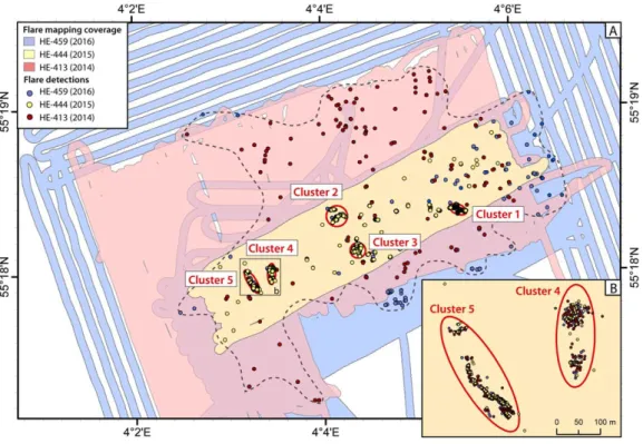
Flares are visible in both the multi- beam and single-beam echosounder data. Due to better resolution and more complete coverage, flare map- ping has been performed using the multibeam data. During the three research cruises, between 490 and 854 flares were detected (Table 1) within an area of about 8 km2 (defined as
‘‘seep-influenced area,’’ Figure 3). Most flares cluster together, and thus we defined five flare clusters numbered 1 to 5 (Figures 2 and 3). The area covered by these five flare clusters is in total about 15,000 m2, correspond- ing to 0.19% of the total seep-influenced area of almost 8 km2. Up to 200 flares occur sparsely scattered around the five flare clusters, which account for 13–21% (range of the three different years) of all detected flares. Flare clusters comprise between 37 (cluster 4) and over 320 (cluster 1) flares in relatively small areas of2000 to 4000 m2(Table 1).
Flares appear in most cases as intense and continuous water column anomalies that often reach the sea sur- face. Such flares are suggested to present constant and steady bubble emission sites. In the flare clusters (except cluster 4), the distance between individual bubble streams was too small for the echosounders to resolve discrete flares, resulting in broad anomalies visible in the echograms. In cluster 4, flares appeared rather discontinuous and incoherent in our data, which might indicate a pulsing and unsteady ebullition of gas bubbles. However, this effect could also result from deflection of the flares with water currents. Flares outside the five clusters appear as individual bubble streams, both in form of intense and continuous anom- alies and relatively weak and/or discontinuous flares. Especially in the northern part of the seep-influenced area, flares appeared pulsing and unsteady. In a recent publication,Urban et al. [2017] present video data
Figure 3.(a) Compilation map showing the flare mapping results of three different years (HE-413 in 2014, HE-444 in 2015, and HE-459 in 2016). The colored areas indicate the flare mapping coverage for each year and corresponding dots the detected flares, respectively. The dashed line outlines the entire defined ‘‘seep-influenced area’’ covering 8 km2. (b) Blow-up of flare clusters 4 and 5 that illustrates the almost identical flare distribution detected during all three years’ surveys within the flare clusters.
Table 1.Size and Number of Flares Per Cluster Area
Subarea
Area Size (m2)
Number of Flares
2014 2015 2016 2016 2016
16.01 13.05 29.03 02.04 Ø
Cluster 1 3040 309 207 320 288 304
Cluster 2 2720 88 50 86 83 85
Cluster 3 1950 79 55 83 80 82
Cluster 4 3930 65 42 37 51 44
Cluster 5 2500 125 73 137 102 120
Surrounding 7.93103 176 63 126 98 112
Total 83103 854 490 789 702 734
acquired during ROV dives at the seafloor at cluster 1 providing a visual impression of the bubble streams and showing their different intensities.
3.1.2. Temporal Variability
In order to evaluate the spatial and temporal variability of the flares, we compared the mapping results of the three cruises with covered areas for flare mapping of 14.9 km2in 2014, 3.6 km2in 2015, and 44.4 km2in 2016. The defined seep-influenced area (8 km2) was 94%, 45%, and 75% surveyed during the three cruises, respectively. However, the five flare clusters were observed and totally insonified every year and only the surrounding area was partially mapped. The number of flares was remarkably similar in 2014 and 2016, whereas generally fewer flares have been counted in 2015 (Table 1). We interpret this observation as an artifact of data quality due to bad weather in 2015. Elevated noise level due to strong ship motion lim- ited the data resolution and hence the flare observations. Also because of the very similar numbers of flares detected in 2014 and 2016, an overall drop in release activity in 2015 seems unlikely.
The largest number of flares was observed in cluster 1 in all three years (Table 1). Cluster 5 ranks second in flare number with about 1/3 of the number of flares as in cluster 1. Clusters 2 and 3 were in all years very similar and cluster 4 had always the smallest number of flares. We performed two almost identical surveys in 2016, which were conducted 4 days apart. This allowed evaluation of the short term variability of flare activity. Results vary by about 11% (3.5–27% for individual flare cluster), whereas the comparison between 2014 and 2016 (averaged) show a difference of 12.5% (1.6–32%). This observation indicates a consistency in seepage activity over days and years in the number of flares within the five flare cluster. In contrast, outside the flare clusters a clear variability was observed with flares rarely being observed twice at the same loca- tion (Figure 3a). Short-term variability might also be the result of a tidal influence on the gas-rich sediments as documented for other seep areas (e.g., Hydrate Ridge [Tryon et al., 1999;Torres et al., 2002], Coal Oil Point [Boles et al., 2001], and offshore Vancouver Island [R€omer et al., 2016]). So far, we lack sufficient data to resolve the influence of tidal pressure changes in our study area.
3.1.3. Methane Flow Rates
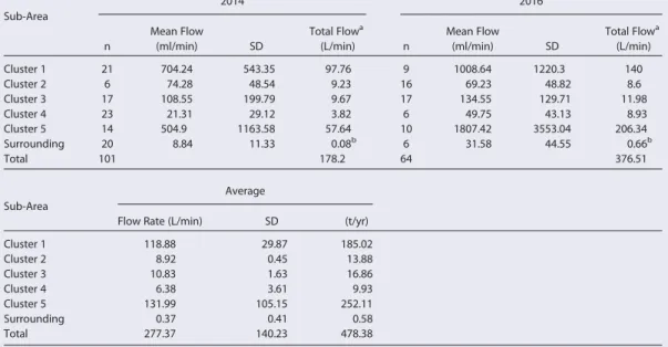
We estimated the amount of methane emitted via gas bubbles in 2014 and 2016. Our estimates are not based on direct video observations in the working area; therefore, we considered a typical bubble size dis- tribution with diameters between 2 and 12 mm as provided byVeloso et al. [2015] (obtained offshore Sval- bard). Also, we used for our estimation bubble rise velocities for clean bubbles [Leifer and Patro, 2002] since we do not have any information about surfactants influencing the bubble rise behavior. Due to these assumptions, a relative error of about 60% and 15%, respectively, was determined byVeloso et al. [2015], which clearly demonstrate the large uncertainties associated with them. Bubble analysis by video observa- tions would be needed to limit the uncertainties and better constrain the methane flow rates. A first quanti- fication of gas flow rate of clusters was done according toVeloso et al. [2015]. The procedure estimates the flow rate of individual flares using an inverse method and subsequently calculates an equivalent flow rate for a group of flares in case the beam footprints of flares overlap each other. The average flow rate of all measurements within the respective clusters was calculated and extrapolated to the cluster area, taking the footprint of the single beam echosounder (with an opening angle of78at a water depth of 43 m resulting in22 m2) into account (see supporting information Figure S2). For each flare cluster and year between 6 and 23 measurements are available (Table 2), resulting in highly variable flow rates from a minimum of 1.7 to a maximum 8593.9 mL/min for individual flares within the clusters (supporting information Table S2).
Converted to the number of bubbles with a typical size distribution as provided byVeloso et al. [2015] such flow rates would equal about 10 to 47,000 bubbles/min. We also estimated flow rates of flares outside the clusters. In contrast to the flare clusters, we extrapolated the resulting flow rate to the number of detected flares and not to the seep-influenced area. Flow rates of these flares are with a maximum of 119.7 mL/min, which is generally lower than flow rates in the flare clusters. The flow rate of all single flares that are located outside the flare clusters is 0.37 L/min (2 years average). Thus, the sum of flow rates of all single flares account for only about 0.1% of the total flow rate, hence, representing a minor contribution to the total gas emission.
Although the flare clusters are clearly the main source of methane to the hydrosphere, large flow rate differ- ences exist between them. In 2014, the estimated flow rates of the clusters scale with the numbers of flares.
Cluster 1 is emitting the most (100 L/min), followed by cluster 5 (50 L/min), clusters 2 and 3 (10 L/min each), and finally cluster 4 with 4 L/min as the weakest contributor (Table 2). In 2016, resulting flow rates for clusters 1, 2, and 3 are relatively similar to those estimated for 2014 (<50% difference). Only cluster 2
showed a decrease of the flow rate; all other flare cluster indicated higher values in 2016 compared to 2014.
Especially cluster 5 was much stronger in intensity and showed the highest flow rate of all flare clusters (200 L/min). Although the number of flares detected within cluster 5 did not change much, it appears that the intensity has increased in 2016 relative to the survey in 2014. The total flow rate of the seep-influenced area was calculated to 178 L/min in 2014 and 377 L/min in 2016, where the difference mainly results from the strong increase of flare cluster 5 in 2016. Although we cannot entirely rule out some methodically produced difference due to two different data sets and changing weather conditions, the error was minimized by using the same hydroacoustic system on the same ship as well as the same settings during postprocessing.
The gas bubbles escaping at the Dutch Dogger Bank seep area are sourced from a biogenic methane reser- voir [Schroot et al., 2005]. Using the ideal gas law under in situ conditions the calculated flow rate corre- sponds to 33–70 mol/min or, assuming constant release, 17–373106mol/yr (corresponding to 273–593 t/yr). Such values are well within the range of published flow rates of (anthropogenic and natural) methane seeps in the North Sea (Figure 4) and indicate the significance of the Dutch Dogger Bank seep area as a main contributor of methane to North Sea water. Based on our estimates, the Dutch Dogger Bank seep area emits more than an order of magnitude more methane than the Tommeliten seep area (26 t/yr) [Schneider von Deimling et al., 2011] and seeps offshore Anvil Point, UK (68 t/yr) [Hinchcliffe, 1987]. Even smaller meth- ane outputs were reported for the Scanner pockmark field in UK Block 15/25 and at Torry Bay, Scotland [Judd et al., 2002]. Furthermore, emission rates have been calculated for a few abandoned wells in the North Sea. The most intensively studied well site is 22/4b, which experienced a blowout in 1990 and still emits large amounts of methane into the North Sea, although with slowly decreasing intensity [Leifer et al., 2015].
Leifer[2015] calculated an annualized emission of 25,000 tons of methane 22 years after the blowout, which is two orders of magnitude larger than all other seepage areas in the North Sea known so far. Three other well sites in the Central North Sea have been investigated byVielst€adte et al. [2015] yielding 1 to 19 t/yr of methane output per well. Hence, well sites represent important contributors to the North Sea methane bud- get comparable to some natural sources, especially having the huge and growing number of abandoned well sites in mind. In relation to seep sites outside of the North Sea, the Dutch Dogger Bank seep area lies on the upper end of methane outputs and is comparable with emission from the Håkon Mosby mud vol- cano (Barents Sea) with 305 t/yr [Sauter et al., 2006] and North Hydrate Ridge (Cascadia Margin) with 350 t/yr [Torres et al., 2002]. Other individual seep sites were estimated to have emission rates between 2 and 91 t/yr, similar to the weaker North Sea seeps (Figure 4). However, the Coal Oil Point seep area emits an
Table 2.List of the Calculated Gas Flow Rates Using FlareHunter and the FlareFlowModule Sub-Area
2014 2016
n
Mean Flow
(ml/min) SD
Total Flowa
(L/min) n
Mean Flow
(ml/min) SD
Total Flowa (L/min)
Cluster 1 21 704.24 543.35 97.76 9 1008.64 1220.3 140
Cluster 2 6 74.28 48.54 9.23 16 69.23 48.82 8.6
Cluster 3 17 108.55 199.79 9.67 17 134.55 129.71 11.98
Cluster 4 23 21.31 29.12 3.82 6 49.75 43.13 8.93
Cluster 5 14 504.9 1163.58 57.64 10 1807.42 3553.04 206.34
Surrounding 20 8.84 11.33 0.08b 6 31.58 44.55 0.66b
Total 101 178.2 64 376.51
Sub-Area
Average
Flow Rate (L/min) SD (t/yr)
Cluster 1 118.88 29.87 185.02
Cluster 2 8.92 0.45 13.88
Cluster 3 10.83 1.63 16.86
Cluster 4 6.38 3.61 9.93
Cluster 5 131.99 105.15 252.11
Surrounding 0.37 0.41 0.58
Total 277.37 140.23 478.38
Note:n, number of measurements.
aMean flow extrapolated to respective total cluster areas as given in Table 1.
bExtrapolated to amount of flares detected in the surrounding area as given in Table 1.
estimated 29,200 t/yr [Hornafius et al., 1999], which is significantly more methane than our study area emits and on the same order of magnitude as the abandoned well 22/4b in the North Sea (Figure 4).
3.2. Subbottom Structures
3.2.1. Sedimentary Sequence in the Study Area
The acquired 50–100 m spaced SBP survey line data allow detailed mapping of sedimentary units and sub- bottom gas indications. Figure 4a shows the typical sedimentary sequence. The lowermost sedimentary unit (Unit 1) is made up of segments of low to high amplitude reflectors. Continuous reflectors and their geometry are hardly visible, probably due to a loss of coherent reflection in coarse-grained sediments. We interpret this unit as Pleistocene glacial deposits, which were deposited during the Last Glacial Maximum (LGM) when the last ice advance reached to this area [Hughes et al., 2016]. The upper boundary of this unit (H1) shows variations in subbottom depth of up to 12 m (Figure 5a). Mapping of H1 reveals a complex pat- tern of depressions in the study area (Figure 6a). A2 km broad depression of up to 12 m depth strikes E-W, shoals and breaks up into a patchwork of lows and highs toward the eastern and western end. The western end of the2 km depression is intercepted by less wide depressions, which strike NWN-SES. The northern continuation branches into two separate arms. Such patterns of depressions in the Pleistocene deposits of the North Sea have been previously interpreted as either glacial tunnel valleys formed beneath the ice sheets covering the area due to melt water flow [Huuse and Lykke-Andersen, 2000;Fitch et al., 2005;
Jørgensen and Sandersen, 2006; Kehew et al., 2012; Janszen et al., 2013] or as fluvial river incisions that formed in front of ice sheets or during ice retreat [Fitch et al., 2005]. Tunnel valleys may show widely varying depths predominantly between 20 and 200 m [Jørgensen and Sandersen, 2006]. However, tunnel valleys and
Figure 4.Compilation of selected seep emission estimates from the seafloor into the water column. Estimates from the literature were put in relation to the quantification presented in this study. Light grey bars show natural, dark grey bars anthropogenic seep sites. The Dutch Dogger Bank seep area emits much more methane than all other known seep sites in the North Sea, besides the abandoned well 22/4b. An ocean wide comparison indicates equivalent emission rates from all seeps in the North Sea with the highest estimate of the Coal Oil Point seep field.
Figure 5.(a) SES subbottom echosounder 4 kHz profile across the seep area. See Figure 6 for location. Pleistocene deposits (Unit 1) show considerable topography at their upper bound- ary (H1). Unit 2 fills the depressions with layered probably marine sediments and is overlain by Unit 3 which is assumed to be modern marine North Sea sediments. High amplitude reflections have been mapped along H1, along two Pleistocene reflectors (R1 and R2) and locally within Unit 2. These gas accumulations underlie the gas seepage clusters and gas migration pathways have been interpreted to be vertical while gas is trapped at individual surfaces along the migration pathway. (b) Close-up of sediment echosounder profile across cluster 1. See Figure 6 for location. High amplitude reflections are visible along H1 as well as within Unit 2 sediments. The pathway of gas through the marine sediments of Unit 2 is acoustically turbid and shows gas accumulations along the migration way as well as directly below the seafloor seep. Note the local overprinting of H1 by gas signatures.
fluvial systems may also occur subsequent to each other during the glacial evolution of the area [Fitch et al., 2005]. We favor the interpretation of subglacial melt water tunnel valleys due to the considerable depth changes along the depression as well as the spatial pattern of the depression, which appears atypical for a river system as it does not show a clear fluvial thalweg as would be expected from a river system.
Unit 2 is made up of medium amplitude reflections that fill the underlying topography of H1 (Figure 5a).
The reflectors indicate concordant sedimentation on top of H1 with decreasing thickness at the flanks of the depressions. In various places outside of the H1 depressions, Unit 2 is not present. Unit 2 is truncated by H2. We interpret this unit as marine sediments deposited during the early Holocene transgression in the area of the southern North Sea. H2 is overlain by Unit 3 that is assumed to consist of modern marine North Sea sediments. Such modern sands or silts have been documented in the North Sea in various places usu- ally with a thickness of only few meters [Konradi, 2000;Zeiler et al., 2000;Stoker et al., 2011].
3.2.2. Gas Indications in the Subseafloor
In addition to the flare detection using the MBES and SBES, gas bubble streams were also visible in the 4 kHz SBP data (Figures 5a and 5b). Gas in the subseafloor is visible as enhanced reflectors and signal blanking underneath these high amplitude reflections; both are due to increased impedance contrasts induced by gas content in the pore-space. High amplitude reflectors attributed to gas in sediments could be mapped pre- dominantly along H1, i.e., the base of Holocene sediments. Either H1 is increased in amplitudes itself or the high amplitude reflector is situated slightly shallower with complete signal blanking underneath (Figures 5a and 5b). This amplitude enhancement in H1, interpreted as accumulated gas at the base of Holocene sedi- ments (Figure 6b), underlies the areas of the vigorously seeping flare clusters (Figures 5a and 5b).
Irregular patches of high amplitudes are visible within the marine sediments of Unit 2 (Figures 5a and 5b).
As sedimentary reflectors do not onlap or drape these high amplitude patches, we assume that they formed after the Holocene deposition. These high amplitudes appear to be individual pockets of gas within the marine sediments, predominantly occurring in the lower part of Unit 2 within the Pleistocene depressions, thus coinciding with maximum thickness of Unit 2 (Figure 6b). Such gas pockets could be another temporary trap for the gas during upward migration from the 600 m deep methane reservoir or
Figure 6.(a) Gridded topography of reflector H1, representing the upper boundary of Unit 1 and thus a late Pleistocene surface before the onset of transgression in the North Sea. The most prominent features are a network of depressions of a depth of10 m below the surrounding area. The nature of this depression is supposed to be a subglacial melt water tunnel valley, which were later filled by marine sediments. (b) Mapping results of different reflectors and gas indications in the sediment echosounder data. Gas accumulations at Pleistocene surfaces can be seen to underlie the gas seepage clusters at the seafloor indicating vertical migration of gas from depth. Local gas pockets within Holocene marine sediments can be seen to coincide with the deepest part of the Late Pleistocene depressions mapped in Figure 6a.
alternatively may present biogenic gas produced in situ where marine sediments have been deposited in sufficient thickness.
Within Unit 1, two reflectors showing enhanced amplitudes have been mapped (R1 and R2 in Figures 5a and 6b). These enhanced reflectors only occur in the central part of the study area (Figure 6b). They underlie large parts of the areas where flares were found. R1 and R2 constitute high amplitude sections of laterally continuous sedimentary reflectors (Figure 5a). We interpret these reflectors as Pleistocene surfaces within Unit 1 where rising gas from depth accumulates before migrating further up to the seafloor. Hence, these reflectors show enhanced amplitudes in areas where gas is ascending through the sediment.
The region of the study area has long been an area of active hydrocarbon exploration. Shallow reservoirs of methane at 600–700 m depth have been recognized in previous studies [Schroot et al., 2005; Stuart and Huuse, 2012]. However, hydrocarbon exploration usually aims for deeper targets in the Paleo and Neogene strata [Kuhlmann and Wong, 2008]. Migration features such as chimneys and seismic blanking have been widely found in the Dutch North Sea sector [Schroot et al., 2005]. Our data show that gas seeping at the Dutch Dogger Bank seep area is fueled from deeper sources and partly accumulate along Pleistocene surfa- ces. This trapping of gas has previously been attributed to the clay content of Pleistocene valley fills [Schroot et al., 2005]. In addition, gas appears to accumulate at the base of the Holocene before finally migrating through the overlying layered marine sediments to escape at the seafloor (Figure 5b). High amplitudes directly beneath the seeps may suggest a very shallow underlying gas reservoir (Figure 5b). However, the locations of the five distinct flare clusters could not be directly related to such shallow subseafloor geologic features. Deeper in the sediment, the locations where gas ascends to the seafloor are determined by salt structures as well as the overlying Pliocene and Pleistocene sedimentation [Kuhlmann and Wong, 2008].
Nevertheless, the establishment of flare clusters in the study area may be facilitated by gas accumulations at Pleistocene surfaces and the base of Holocene sedimentation, allowing gas accumulation and continuous supply of gas to the seafloor from such shallow reservoirs in only few meters sediment depth.
Flares have been found in significant number above Unit 2 sediments predominantly around and to the North of cluster 1 (Figure 3). This area does not show one of the enhanced reflectors R1 or R2 but has abun- dant gas pockets within Unit 2 (Figure 6b). This area is also characterized by the maximum thickness of Unit 2 sediments (Figure 6a). Therefore, we speculate that individual flares in this area may be fed from small iso- lated gas pockets in Holocene sediments rather than by gas rising from depth. Gas release in the study area may thus originate from two different gas sources, one deeper source feeding the five flare clusters and one shallow source supplying individual flares overlying the maximum thickness area of Unit 2.
3.3. Atmospheric Methane Contribution
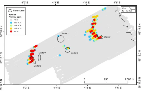
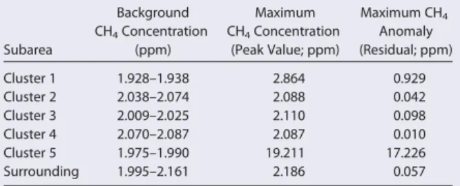
Continuous air measurements showed elevated methane concentrations above individual flare clusters (Fig- ures 7 and 8), clearly pointing to a contribution of methane from seafloor seepage to the atmosphere.
Methane peaks with values of up to 19.21 ppm methane (10 times background) have been measured (Table 3). The highest methane concentrations of 19.21 and 2.86 ppm were located above clusters 5 and 1, respec- tively. Smaller anomalies of 2.11 and 2.09 ppm were detected at clusters 3 and 2, respectively. No indica- tions for increased atmospheric concentrations have been found above cluster 4 (Figure 8). A detailed survey running 10 lines in E-W direction with 20 m line spacing was conducted at cluster 1, illustrating a good correlation of the methane peaks with the flare distribution (Figure 7). The background methane con- centration was 1.94 ppm and distinct peaks with values 0.20–0.92 ppm higher were measured during lines 1–5, and 7, i.e., the more northern lines crossing the flare cluster (Figure 7). The wind direction was north- ward with wind speeds between 4 and 5 m/s, thus methane transported from the seafloor and entering the atmosphere should have drifted with the wind. Transport of methane with the wind was also apparent in the data set that covered the central part of the seep-influenced area with all flare clusters (Figure 8). Meth- ane anomalies were found at the north western side of the flare clusters. Especially the more intense emis- sions at clusters 1 and 5 illustrate the wind drift; highest values occurred just above the flares decreasing to still measurable anomalies of 0.06 ppm more than 800 m in wind direction northward from cluster 1 (at the same height of2 m above sea surface).
Judd[2015] presented data using a similar method measuring sea surface atmospheric methane concentra- tions during a survey crossing the southern and central North Sea and identified 15 anomalies associated with natural or petroleum industry sources. One pronounced anomaly has been detected close to the Dutch
Dogger Bank seep area, and it was speculated that this relates to the A12-A or B13-A (our study area) gas production platforms [Judd, 2015]. However, due to the opposite wind direction the anomaly seems more likely to be associated with another as yet unrecognized natural gas seep or a closely located abandoned well [Judd, 2015]. Although our data are limited, the observed atmospheric methane anomaly originating from flare cluster 1 is only measurable less than 1 km away from the seep, favoring the suggestion that a plume from the Dutch Dogger Bank seep area will probably not be detectable more than 10 km away even with higher wind speeds or temporally increased seafloor release.
Another independent observation that the Dutch Dogger Bank seep area transports methane through the water column close to the sea surface was presented bySchneider von Deimling et al. [2015], who measured higher surface water concentrations during transit from the German coast to UK Block 22/4b and also cross- ing the Dogger Bank.
Figure 7.(a) Map showing the flares detected within and around flare cluster 1 in 2016 and the location of the 10 east-westward directed survey lines. (b) Time series plot of the air methane concentrations measured with the GGA during the survey. White parts indicate the times along the 10 survey lines, grey areas cover the time when the ship turned.
Figure 8.Map of the area covered during the survey on 2 April 2016 (HE-459) showing air methane anomalies relative to the locations of the five flare clusters. Only flare clusters 1 and 5 show high methane anomalies, which are apparently drifting with the wind, which was directed northward at the beginning of the survey (north-western part) and rotated to the west during the second part (south-east).
3.3.1. Bubble Dissolution Modeling In order to evaluate if bubble streams with a typical bubble size distribution (as used for quantification with the FlareFlowMod- ule) would reach the sea surface and trans- port methane directly into the atmosphere through a40 m deep water column, we applied the Single Bubble dissolution model (SiBu-GUI) [Greinert and McGinnis, 2009] by implementing ambient water pro- files derived from CTD casts during HE-459.
The modeled results of the bubble fate (supporting information Figure S3) support our observations as: (a) all bubbles larger than 2.7 mm in diameter would reach the sea surface and (b) bubbles with diameters
>4 mm could transport some fraction of the initial methane emitted at the seafloor into the atmosphere.
Our data show that even weaker and individual bubble streams can be followed in echograms through the entire water column. Although only parts of the initially released methane is still in the bubbles when reach- ing the sea surface, the most intense flare clusters show a methane plume detectable in the atmosphere.
Taking the bubble size distribution into account (2–15 mm in diameter, average6 mm, SD52.1 mm, as provided byVeloso et al. [2015], about 20.6% of the initial methane fraction would be transported directly to the atmosphere, which is (assuming 100% methane content of the initially released bubbles) about 57.14 L/min (or 21.7 t/yr calculated after the ideal gas law at atmospheric pressure) from the entire seep area. If we extrapolate the gaseous flux of methane over the seep-influenced area (8 km2), we get a flux of 5.31 nmol/s/m2. This gaseous methane flux is larger than the dissolved methane flux of the area during win- ter (1.2 nmol/s/m2), and even an order of magnitude higher compared to the dissolved methane flux in summer (0.1 nmol/s/m2), when a thermocline constrains dissolved methane to the deeper water column [Mau et al., 2015]. Our results illustrate that methane can directly be transported by bubbles through the water column from locally confined but intense bubbling seep areas.
Furthermore, the SiBu-GUI does not account for possibly occurring upwelling processes within the bubble seeps, which would increase the fraction of methane entering the atmosphere. Enhanced seepage- mediated atmospheric methane input has been attributed to vertical upwelling of gas plumes even from greater depth [Leifer et al., 2006]. The involved upwelling processes also have been shown to occur at the North Sea blowout site UK22/4b, where dye tracer injections revealed gas plume rise velocities up to 1 m/s near the seabed in100 m water depth [Leifer et al., 2015;Schneider von Deimling et al., 2015]. At that loca- tion, the amount of methane reaching the sea surface has been estimated to 7006300 t/yr [Schneider von Deimling et al., 2015], which (although still two orders of magnitude higher than the value presented in this study) was less than the authors predicted for this intense emission site.Schneider von Deimling et al. [2015]
also present a possible explanation derived from a 3-D multibeam water column analysis, indicating a spiral vortex of the bubble plume as an additional process slowing down the bubble rise.Leifer et al. [2015] addi- tionally suggest a unique ‘‘megaplume’’ related process enhancing individual bubble gas exchange rate at seeps emitting>106L/d. Although still to be tested at other seep sites of different intensities, such observa- tions indicate the complexity of bubble plume dynamics and the need for further investigations to improve the existing model results.
Our data on the atmospheric methane concentrations were derived during early spring time, when no strat- ification of the water column existed. A density stratification might, however, limit vertical transport, as, e.g., at the 70 m deep Tommeliten seep area, whereSchneider von Deimling et al. [2011] could show that a sum- mer thermocline constrains methane transport to the atmosphere.Mau et al. [2015] presented CTD hydro- cast data that show that our study area is becoming stratified in summer, too, which might decrease the atmospheric methane contribution in our study area in summer as well.
4. Conclusion
We used a multidisciplinary approach to investigate the subseafloor distribution of gas, gas bubble emis- sions in the water column, and atmospheric methane concentrations. This approach provided a
Table 3.Atmospheric CH4Concentrations (Greenhouse Gas Analyzer) as Measured in 2016
Subarea
Background CH4Concentration
(ppm)
Maximum CH4Concentration
(Peak Value; ppm)
Maximum CH4
Anomaly (Residual; ppm)
Cluster 1 1.928–1.938 2.864 0.929
Cluster 2 2.038–2.074 2.088 0.042
Cluster 3 2.009–2.025 2.110 0.098
Cluster 4 2.070–2.087 2.087 0.010
Cluster 5 1.975–1.990 19.211 17.226
Surrounding 1.995–2.161 2.186 0.057
comprehensive view of the relation between gas supply in the sediment and its relation to flare occurrence at the seafloor as well as the transport of methane from the seafloor into the atmosphere:
1. By far the most methane is emitted through flares clustering close together in five distinct areas of 2000–4000 m2each, although the seep-influenced area covers in total8 km2.
2. The five flare clusters are all related to gas accumulations in the shallow subseafloor at the top of the late Pleistocene deposits, which sustain continuous methane supply to the water column. Individual pulsing gas emissions, in contrast, appear sourced by gas pockets in Holocene channel infills and could point to more recent in situ biogenic methane production. Gas sampling for carbon isotopic analysis might help to finally evaluate if flare cluster and pulsing flares above Holocene channel infills can be divided and attributed to different methane formation processes and sources.
3. The amount of emanating methane was estimated from echosounder backscatter information using FlareHunter and FlareFlowModule [Veloso et al., 2015]; this resulted in values higher than at other natural seeps in the North Sea, but comparable to other prominent seep sites, e.g., the Håkon Mosby mud vol- cano or Northern Hydrate Ridge. However, we predict large uncertainties in the estimate due to the assumed bubble size distribution (60% relative error) and rise rates (15% relative error). Visual sea- floor data would be needed to verify our results.
4. We found elevated methane concentrations in the atmosphere, which might be attributed to bubble mediated transport through the40 m water column. Methane anomalies were clearly restricted to the two most intense flare clusters and were not apparent in the rest of the seep-influenced area. Thus we can establish a flux limit above which seeps certainly contribute methane to the atmosphere, taking into account the water depth and oceanographic conditions. Flare clusters emitting less than 20 L/min appear not to transport much methane to the atmosphere, whereas those with fluxes>100 L/min clearly do transport sufficient methane to the atmosphere to be detectable with our methods. Direct bubble transport or sea/air gas exchange of the dissolved gas phase contributes to this flux but the magnitude of those contributions is hardly constrained.
5. Repeated analysis of three consecutive years revealed spatial similarities of seep clusters, but heterogene- ities in emission intensities. Results indicate that data acquired during cruises, which represent only snap- shots in time, can result in twice as high methane emission rates between different years. Long-term monitoring would be needed to better constrain the magnitude of variability on different time scales.
References
Artemov, Y. G., V. N. Egorov, G. G. Polikarpov, and S. B. Gulin (2007), Methane emission to the hydro- and atmosphere by gas bubble streams in the Dnieper Paleo-delta, the Black Sea,Mar. Ecol. J.,6, 5–26.
Boles, J. R., J. F. Clark, I. Leifer, and L. Washburn (2001), Temporal variation in natural methane seep rate due to tides, Coal Oil Point area, California,J. Geophys. Res.,106(C11), 27,077–27,086.
Borges, A. V., W. Champenois, N. Gypens, B. Delille, and J. Harlay (2016), Massive marine methane emissions from near-shore shallow coastal areas,Sci. Rep.,6, 27908.
Caress, D. W., and D. N. Chayes (1996), Improved processing of hydrosweep DS multibeam data on the R/V Maurice Ewing,Mar. Geophys.
Res.,18(6), 631–650.
Fitch, S., K. Thomson, and V. Gaffney (2005), Late Pleistocene and Holocene depositional systems and the palaeogeography of the Dogger Bank, North Sea,Quat. Res.,64, 185–196.
Greinert, J. (2008), Monitoring temporal variability of bubble release at seeps: The hydroacoustic swath system GasQuant,J. Geophys. Res., 113, C07048, doi:10.1029/2007JC004704.
Greinert, J., and D. F. McGinnis (2009), Single bubble dissolution model—The graphical user interface SiBu-GUI,Environ. Model. Software, 24, 1012–1013, doi:10.1016/j.envsoft.2008.12.011.
Greinert, J., D. F. McGinnis, L. Naudts, P. Linke, and M. De Batist (2010), Atmospheric methane flux from bubbling seeps: Spatially extrapo- lated quantification from a Black Sea shelf area,J. Geophys. Res.,115, C01002, doi:10.1029/2009JC005381.
Hinchcliffe, J. C. (1978), Death stalks the secret coast,Triton,23(2), 56–57.
Hornafius, J. S., D. Quigley, and B. P. Luyendyk (1999), The world’s most spectacular marine hydrocarbon seeps (Coal Oil Point, Santa Barbara Channel, California): Quantification of emissions,J. Geophys. Res.,104(C9), 20,703–20,711.
Hovland, M. (2007), Discovery of prolific natural methane seeps at Gullfaks, northern North Sea,Geo-Mar. Lett.,27, 197–201.
Hovland, M., and H. Svensen (2006), Submarine pingoes: Indicators of shallow gas hydrates in a pockmark at Nyegga, Norwegian Sea,Mar.
Geol.,228(1–4), 15–23.
Hovland, M., H. Svensen, C. F. Forsberg, H. Johansen, C. Fichler, J. H. Fosså, R. Jonsson, and H. Rueslåtten (2005), Complex pockmarks with carbonate-ridges off mid-Norway: Products of sediment degassing,Mar. Geol.,218, 191–206.
Hughes, A. L. C., R. Gyllencreutz, Ø. S. Lohne, J. Mangerud, and J. I. Svendsen (2016), The last Eurasian ice sheets—A chronological database and time-slice reconstruction, DATED-1,Boreas,45, 1–45.
Huuse, M., and H. Lykke-Andersen (2000), Overdeepened quaternary valleys in the eastern Danish North Sea: Morphology and origin, Quat. Sci. Rev.,19, 1233–1253.
Acknowledgments
We greatly appreciate the shipboard support from the master, crew, and scientists of the research vessel HEINCKE during HE-413, HE-444, and HE-459. We want to express our gratitude to Stefanie Buchheister, Dawid Dabrowski, and Torben Gentz for technical support of the ICOS system for cruise HE-459. Furthermore, we thank Paul Wintersteller, Christian dos Santos Ferreira, Jan-Hendrik K€orber, Heiko Sahling, and Stefanie Gaide for their help during the hydroacoustic acquisition on board and processing of the multibeam data.
Data acquired for this study are available through the World Data Center PANGAEA. We thank IHS Global Inc. (The Kingdom Software) for providing academic software licenses for data interpretation. This work was partly funded through the DFG- Research Center/Excellence Cluster
‘‘The Ocean in the Earth System’’ and mainly financed through the research program ‘‘IMGAM—Intelligent Monitoring of Climate Wrecking CO2/ CH4Emissions in the Sea’’ of the Federal Ministry for Economic Affairs and Energy (BMWi project 03SX346B).
Susan Mau is funded by the DFG project ‘‘Limitations of Marine Methane Oxidation’’ (MA 3961/2–1). Finally, we thank the editor Janne Blichert-Toft and four anonymous reviewers for providing contructive comments that helped to improve the paper.