energies
Article
Thermal State of the Blake Ridge Gas Hydrate Stability Zone (GHSZ)—Insights on Gas Hydrate
Dynamics from a New Multi-Phase Numerical Model
Ewa Burwicz * and Lars Rüpke
GEOMAR Helmholtz Centre for Ocean Research Kiel, Wischhofstrasse 1-3, D-24148 Kiel, Germany
* Correspondence: eburwicz@geomar.de
Received: 5 June 2019; Accepted: 24 August 2019; Published: 3 September 2019 Abstract:Marine sediments of the Blake Ridge province exhibit clearly defined geophysical indications for the presence of gas hydrates and a free gas phase. Despite being one of the world’s best-studied gas hydrate provinces and having been drilled during Ocean Drilling Program (ODP) Leg 164, discrepancies between previous model predictions and reported chemical profiles as well as hydrate concentrations result in uncertainty regarding methane sources and a possible co-existence between hydrates and free gas near the base of the gas hydrate stability zone (GHSZ). Here, by using a new multi-phase finite element (FE) numerical model, we investigate different scenarios of gas hydrate formation from both single and mixed methane sources (in-situ biogenic formation and a deep methane flux). Moreover, we explore the evolution of the GHSZ base for the past 10 Myr using reconstructed sedimentation rates and non-steady-state P-T solutions. We conclude that (1) the present-day base of the GHSZ predicted by our model is located at the depth of ~450 mbsf, thereby resolving a previously reported inconsistency between the location of the BSR at ODP Site 997 and the theoretical base of the GHSZ in the Blake Ridge region, (2) a single in-situ methane source results in a good fit between the simulated and measured geochemical profiles including the anaerobic oxidation of methane (AOM) zone, and (3) previously suggested 4 vol.%–7 vol.% gas hydrate concentrations would require a deep methane flux of ~170 mM (corresponds to the mass of methane flux of 1.6×10⁻¹¹ kg s−1m−2) in addition to methane generated in-situ by organic carbon (POC) degradation at the cost of deteriorating the fit between observed and modelled geochemical profiles.
Keywords: gas hydrate; numerical modeling; methane; Blake Ridge
1. Introduction
Gas hydrates (clathrates) are ice-like crystalline cage structures containing various greenhouse gases such as methane or CO2, which are stored within their crystallographic structure. The combination of low-temperature and high-pressure conditions defines the gas hydrate stability zone (GHSZ), which is a proxy to the abundance of gas hydrates in marine sediments. Marine gas hydrate deposits were discovered mainly along continental margins (slope and rise) where water depths exceed ~300 m and bottom water temperatures are sufficiently low. Their potential impact on climate change [1–4], slope stability [5,6], and global energy reserves [7–9] have drawn considerable public and scientific attention over the last decades. Yet, the amount of gas hydrates present on a global scale is still under debate [7,10,11]. Several numerical models of a different complexity have been developed to estimate the potential amounts of clathrates within marine sediments [12–17]. Global estimates range from 500 Gt up to 75,000 Gt of carbon and show a variation of several orders of magnitude. In comparison, the world’s conventional gas endowment has been estimated at 2.567 TBOE (trillion barrels of oil equivalent)=0.436×10¹⁵m3of natural gas [18], which is about 0.5%–40% of the total methane gas
Energies2019,12, 3403; doi:10.3390/en12173403 www.mdpi.com/journal/energies
volume potentially trapped in gas hydrates (from 1.06×10¹⁵m3CH4up to 120.78×10¹⁵m3CH4at STP condition).
One of the best-known gas hydrate provinces, the Blake Ridge Site offshore South Carolina, has been widely investigated during the Ocean Drilling Program (ODP) Leg 164. Seismic profiles across two (995 and 997) out of the three (955, 997, and 994) drill sites show clearly defined BSRs sub-parallel to the seafloor. Their seismic signature is characteristic for the boundary between free gas- and hydrate-bearing sediments in that high-amplitude seismic reflections (corresponding to the presence of a free gas) are overlain by low-amplitude seismic reflections, which is known as the
‘blanking effect’ [19]. The depth of a seismic BSR typically corresponds to the base of the GHSZ, which defines the sharp phase boundary between the stability fields of gas hydrate and free gas. However, at the Blake Ridge province, BSR depths at the 995 and 997 sites (~440–450 mbsf) do not correspond with the bottom of the thermodynamic GHSZ (~520 mbsf) [20–22]. It has been suggested that this discrepancy is caused by a co-existence of free gas and hydrate within the GHSZ. The seismic data appears to be consistent with such a co-existence of phases, which allows for the possibility of free methane gas migration within the GHSZ [20,23,24]. However, free gas becomes the wetting phase when co-existing with pore fluids, so that it is generally assumed that a relatively high free gas concentration, possibly from a deep thermogenic source, is required to initialize such a process although the source of such flux is still debatable. Several studies have pointed to the possibility that a deeply sourced upward methane flux is involved in the formation of Blake Ridge gas hydrates [25,26]. Following this hypothesis, the potential rate of pore fluid flux into the GHSZ has been calculated from halogen geochemical analysis [27] and was estimated at 0.2 mm·year−1but such geochemically inferred flux estimates remain debated. Support for a deep fluid/methane flux also comes from previous modeling attempts [25–31], which failed to reproduce sufficiently high hydrate and free gas concentrations when assuming a single biogenic source of methane, constant sedimentation rates over the entire history of the basin, and no additional deep methane flux. Paradoxically, the inferred deep methane flux is inconsistent with the strongly depletedδ13C isotopic signature of methane gas at the Blake Ridge Site [32], which points to a purely microbial in-situ gas hydrate origin [22,33].
Here, by applying a new numerical model that overcomes some restrictions of previous modeling attempts such as allowing for variable sedimentation rates and seafloor organic carbon (POC) concentrations through time, we investigate (1) if the Blake Ridge gas hydrates could have formed from a single in-situ microbial source or rather from a mixed source (microbial+deep-sourced methane flux), (2) the discrepancy between the observed BSR depth and theoretical base of the GHSZ, and (3) the impact of variations in sediment deposition and compaction on fluid and gas flow regimes coupled with bio-chemical reactions occurring within the sediment column.
1.1. The Blake Ridge Site Geological Setting and Characterization
The Blake Ridge is situated offshore from the southeastern US coast (South Carolina) as a stable Neogene and Quaternary sediment drift deposit (Figure1). Sediment wave structures along the Blake Ridge southern flanks result from the presence of the Gulf Stream that mixes with the Western boundary undercurrent (WBUC) at moderate bottom water depths [34]. Since this area is strongly influenced by the Gulf Stream, it is particularly vulnerable to changes in ocean circulation that might occur under a warming climate. Large quantities of methane gas hydrates locked within Blake Ridge sediments contribute to the discussion on submarine slope failure scenarios and other natural hazards that might take place if the hydrate reservoir becomes unstable [3,35,36]. Sediments at the Blake Ridge are mostly homogenous and contain mostly clays, claystones, and fine-grained mudstones [20] that were deposited at relatively high sedimentation rates [37].
The Blake Ridge Site is characterized by low fluid advection rates and a mostly homogenous sediment composition with clay fractions of 60%–70% and limited changes in a grain size over the entire depth profile [20]. At present, sediments are deposited with an organic carbon content that generally varies between 0.5 wt.%–1 wt.% [22] with maximum values of up to 1.6 wt.% [20,33], which is typical
Energies2019,12, 3403 3 of 24
for organically rich oceanic margin sediments. The source of sedimentary organic matter at Sites 994, 996, and 997 has been described as mainly marine [38]. Rapid burial of organic matter has probably resulted in the high preservation of POC with depth in the Blake Ridge region. Isotopically lighter terrestrial POC might be additionally transported into the system from the neighboring continental shelf. The isotopic composition of low molecular-weight hydrocarbons (methane and ethane) suggest a microbial origin (δ13CCH4values more negative than−61%). According to the relationship between δ13CCH4 andδDCH4 values, the production of methane occurred via CO2 reduction at all Leg 164 Sites [38] and the pools of CH4and CO2were decoupled from each other, which implies an open carbon system during diagenetic processes.
Energies 2019, 12, 3403 3 of 24
is typical for organically rich oceanic margin sediments. The source of sedimentary organic matter at Sites 994, 996, and 997 has been described as mainly marine [38]. Rapid burial of organic matter has probably resulted in the high preservation of POC with depth in the Blake Ridge region. Isotopically lighter terrestrial POC might be additionally transported into the system from the neighboring continental shelf. The isotopic composition of low molecular-weight hydrocarbons (methane and ethane) suggest a microbial origin (δ13CCH4 values more negative than −61‰). According to the relationship between δ13CCH4 and δDCH4 values, the production of methane occurred via CO2
reduction at all Leg 164 Sites [38] and the pools of CH4 and CO2 were decoupled from each other, which implies an open carbon system during diagenetic processes.
Figure 1. Bathymetric map of the Blake Ridge gas hydrate province including drill Site locations of Ocean Drilling Program (ODP) Leg 164 (modified after Dillon and Paull [39]). Bathymetry contours are presented in meters. The shaded area (in pink) depicts the BSR occurrence.
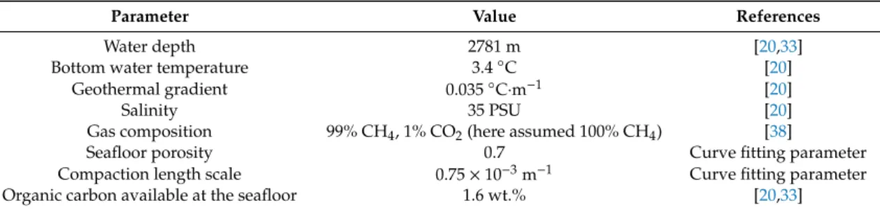
Based on the SO4 profiles, it was postulated that anaerobic oxidation of methane (AOM) is the main process responsible for sulfate depletion at the Blake Ridge province [33]. The boundaries of the sulfate-presence-zone range from the seafloor to ~20 mbsf or ~23 mbsf and appears to be primarily controlled by the flux of methane from underlying sediments rather than organic matter supply from the top [33]. Gas hydrate deposits at the Blake Ridge province are mainly represented by structure I hydrates with 94% cage occupancy and volumetric gas to water ratio of ~204, which corresponds to a hydration number of n = 6.1 calculated for in-situ pressure conditions at the Blake Ridge. Table 1 contains the general characteristics of Site 997, which has been chosen as a benchmark site for this numerical study. Data included in Table 1 were previously established from drilling reports, seismic data interpretations, and other sources.
Table 1. Blake Ridge Site 997 characterization.
Parameter Value References
Water depth 2781 m [20,33]
Bottom water temperature 3.4 °C [20]
Geothermal gradient 0.035 °C·m−1 [20]
Salinity 35 PSU [20]
Gas composition 99% CH4, 1% CO2 (here
assumed 100% CH4) [38]
Seafloor porosity 0.7 Curve fitting parameter
Compaction length scale 0.75 × 10⁻³ m−1 Curve fitting parameter Organic carbon available at the seafloor 1.6 wt.% [20,33]
Figure 1.Bathymetric map of the Blake Ridge gas hydrate province including drill Site locations of Ocean Drilling Program (ODP) Leg 164 (modified after Dillon and Paull [39]). Bathymetry contours are presented in meters. The shaded area (in pink) depicts the BSR occurrence.
Based on the SO4profiles, it was postulated that anaerobic oxidation of methane (AOM) is the main process responsible for sulfate depletion at the Blake Ridge province [33]. The boundaries of the sulfate-presence-zone range from the seafloor to ~20 mbsf or ~23 mbsf and appears to be primarily controlled by the flux of methane from underlying sediments rather than organic matter supply from the top [33]. Gas hydrate deposits at the Blake Ridge province are mainly represented by structure I hydrates with 94% cage occupancy and volumetric gas to water ratio of ~204, which corresponds to a hydration number of n=6.1 calculated for in-situ pressure conditions at the Blake Ridge. Table1 contains the general characteristics of Site 997, which has been chosen as a benchmark site for this numerical study. Data included in Table1were previously established from drilling reports, seismic data interpretations, and other sources.
Table 1.Blake Ridge Site 997 characterization.
Parameter Value References
Water depth 2781 m [20,33]
Bottom water temperature 3.4◦C [20]
Geothermal gradient 0.035◦C·m−1 [20]
Salinity 35 PSU [20]
Gas composition 99% CH4, 1% CO2(here assumed 100% CH4) [38]
Seafloor porosity 0.7 Curve fitting parameter
Compaction length scale 0.75×10⁻³m−1 Curve fitting parameter
Organic carbon available at the seafloor 1.6 wt.% [20,33]
To understand the depositional history at the Blake Ridge province, detailed studies on nannofossils and sedimentary particles have been performed [37]. According to the authors, productivity regimes at the Blake Ridge Site 997 can be divided into five distinct stages: Low-productivity stage 1 from 6.6 Ma to 6 Ma, high-productivity stage 2 from 6 Ma to 4.8 Ma, low-productivity stage 3 from 4.8 Ma to 3.6 Ma, fluctuating productivity stage 4 from 3.6 Ma to 0.8 Ma, and the final low-productivity stage 5 from 0.8 Ma to present. These data imply a down-core increase in sedimentation rates (see Table2), which has been used as an input dataset for our modeling runs.
Table 2.Rates of sediment accumulation at Blake Ridge Site 997 after Ikeda et al. [37].
Epoch Age (Ma) Value (mm·yr−1) Sediment Depth after Compaction (mbsf) Pleistocene
0–0.53 0.235 0–18
0.53–1.26 0.105 18–48
1.26–1.65 0.220 48–70
Pliocene
1.65–2.51 0.140 70–110
2.51–2.55 0.010 110–118
2.55–2.76 0.145 118–151
2.76–3.62 0.180 151–308
3.62–3.72 0.155 308–324
3.72–4.43 0.205 324–339
4.43–4.97 0.055 339–415
Late Miocene
4.97–5.59 ~0.060 415–552
5.59–5.92 ~0.005 552–588
5.92–6.6 ~0.025 588–750
1.2. Depth Discrepancy between the Observed BSRs and the Base of the GHSZ at Sites 995 and 997
A sharp BSR is present at a depth of ~440–450 mbsf at ODP drill Sites 995 and 997 [20]. The seismic signatures start to differ between the two Sites below the BSRs at depths between 440 and 530 mbsf, where the dipole waveform amplitudes have relatively high values at Site 977 and low values at Site 995, giving clear indications for differences in elastic properties [20]. Detailed analysis of a core from ODP Site 995 provide direct information on gas hydrate and free gas concentrations as well as a possible mixing zone of these two phases [21]. Indications for the presence of gas hydrates were found in the depth interval ~200–440 mbsf via core thermal measurements, chemical analysis, and sediment samples recovered using pressure core sampler (PCS) [20,40]. Moreover, high gradients in seismicVp/Vswave speeds point to gradients in sediment consolidation possibly related to hydrate crystallization. A strong decrease inVpwas found between depth of ~440 mbsf down to ~520 mbsf, which is a good indication for the presence of free gas. However, it has been reported [21] that parallel to theVpdecrease, no drop inVp/Vswas found, which was judged as unusual pointing to changes in mechanical properties. The authors discuss the possibility of gas hydrate dissociation over this interval to explain the differences in sediment consolidation with depth. The deepest analyzed section (>~520 mbsf) shows no hints for the presence of gas hydrates and is characterized by a significant decrease inVp/Vsconsistent with the presence of free gas.
Contrary to the indirect observations, thermal and chemical analysis of the core from Site 995 did not indicate gas hydrate presence deeper than ~440 mbsf. However, the base of the thermodynamic GHSZ (based on theoretical steady-state calculations) is deeper at ~540 mbsf [21]. Several authors gave hypothetic explanations for this GHSZ thickness discrepancy suggesting that strong capillary forces arising in the fine-grained sediments might move the BSR up [41,42]. As a consequence of the developing capillary forces, gas hydrate may preferentially dissociate in the smaller sediment pores, which would allow for the co-existence of free methane gas and gas hydrates in bigger sediment pores.
Gas hydrates were present in the Site 997 core at depths from ~180 to ~240 mbsf and from ~380 to ~450 mbsf [20,24]. Hydrate concentrations estimated from the ODP drilling results are relatively low at ~4%–7% [20,27] and an external upward fluid flow of approximately 0.2 mm·year−1 was
Energies2019,12, 3403 5 of 24
inferred [27] based on measured Br−/I−ions ratios. However, the above estimates on gas hydrate saturation are based on indirect methods (e.g., chlorinity and salinity measurements) and remain debatable. Thickness of the thermodynamic GHSZ extends to ~500 mbsf and does not match the depth of the BSR (~450 mbsf) [21]. A hypothesis of gas hydrate and free gas co-existence in the overlapping interval (450 mbsf–500 mbsf) might be applicable to this site with some additional comments: As it was reported by Guerin et al. [21], only a 40 m thick interval below 450 mbsf has some indications for free gas presence. Monopole waveforms of the deeper part of this section remain not attenuated.
Therefore, the discrepancy between observed BSR depth and theoretical GHSZ suggests a non-steady state situation.
1.3. Previous Modeling Approaches of the Blake Ridge Site 997
Previous modeling attempts to investigate the dynamics of gas hydrate formation at Blake Ridge Site 997 have been conducted by several authors [25,26,29–31,43]. The potential of gas hydrate crystallization and distribution was investigated [29] for diffusion versus advection-dominated systems using a steady-state analytical model. According to these findings, a sufficiently high methane mass flux of about 3×10⁻¹¹kg s−1m−2at the bottom of the GHSZ is required for hydrate accumulations to extend down to the base of the theoretical GHSZ [29]. In that case, a quasi-steady state was obtained after 10 Myr simulation time. They concluded that the observed surface POC fraction of 1.5 wt.%
results in an average hydrate fraction of about 2 vol.%, which is lower than the inferred gas hydrate concentrations (4 vol.%–7 vol.% after Paull et al. [20]). Thus, a significant methane supply from underlying sediments was required to match the field observations. The dynamics of gas hydrate formation were investigated [30,31] in terms of (1) a constant upward fluid velocity of about 0.26 mm year−1and (2) fluid flow restricted to 0.08 mm year−1and in-situ biogenic methane source with 50%
conversion of the available organic carbon. This numerical approach did not contain a bacterial sulfate reduction zone. The first scenario resulted in 3 vol.% of gas hydrates and 2 vol.% of free gas occupying the pore space, whereas the second one led to 5 vol.% and 3 vol.% of gas hydrates and free gas, respectively. Integrating AOM reaction into the model [31] showed that a good fit of modeled sulfate curves occurs for the first scenario assuming a high upward flux of the fluid phase. Although it has been concluded that the anaerobic oxidation of methane is the dominant reaction leading to sulfate depletion at the Blake Ridge Site, it was apparently difficult to obtain a fit between model predictions and observed chloride and sulfate concentrations. A complex study on gas hydrate dynamics at the Blake Ridge Site was conducted [26] incorporating the entire biogeochemical datasets of dissolved bromide, ammonium, iodide, sulfate, total nitrogen, and organic carbon available at the seafloor. Moreover, this modeling approach contained a novel reaction rate for in-situ biogenic methane formation that links the concentration of degradable organic carbon to the concentration of dissolved methane and inorganic carbon via Monod inhibition rates and age-dependent kinetics. POC concentration at the seafloor were kept constant (1.6 wt.%) for the first period of 5 Myr and then, subsequently, lowered to 0.65 wt.% for the last 0.7 Myr. The best fit to the geochemical profiles was obtained for interstitial fluid velocities of 0.12 mm year−1calculated at the sediment surface and assuming an additional low upward fluid flux at the base of the model. However, gas hydrate concentrations obtained in this case were one order of magnitude lower (about 0.6 vol.%) than observed at that site. Presence of gas bubbles ascending from the deep origin has been proposed as an explanation for higher hydrate concentrations reported from the field. A series of modeling scenarios for a Blake Ridge Site were presented [25]
including only in-situ methane generation, prescribed flux of dissolved methane through a lower boundary (fluid mass of 9×10⁻⁹kg s−1m−2), or a mixed methane source (in-situ generation plus 40%
of previous fluid mass flux). It was concluded that in-situ methane generation alone does not explain gas hydrate concentrations observed in the Blake Ridge and, moreover, an upward fluid flux applied in the second scenario corresponds to the seafloor fluid velocities of about 0.28 mm year−1, which remains too high in comparison to the deduced interstitial fluid velocities [27]. The third modeling scenario assuming mixed methane source stays in good agreement with reported seafloor velocities
and the average gas hydrate concentrations obtained in this case are about 5 vol.%, however free gas concentrations not exceeding 3 vol.%–4 vol.% seem to be too low with respect to the observations.
2. Materials and Methods 2.1. Mathematical Model 2.1.1. Introduction
The new numerical multi-phase model simulates gas hydrate and free gas formation from both in-situ POC degradation and a deeply sourced methane flux. The model contains four phases (solid porous matrix, pore fluids, gas hydrate, and gaseous methane (CH4gas)) and four chemical species (organic carbon (POC), dissolved inorganic carbon (DICdiss), dissolved methane (CH4diss), dissolved sulfates (SO4diss)). The model resolves four key bio-chemical processes in anoxic marine sediments: (1) POC degradation, (2) sulfate reduction, (3) methanogenesis, and (4) anaerobic oxidation of methane (AOM). Sediment pore space can be occupied by three phases (pore fluids carrying chemical species, solid gas hydrates, and free methane gas). Gas hydrate present in the pore space is assumed stationary with respect to the grains and is transported with the burial velocity of sediments. Formation of gas hydrate and free gas takes place whenever the concentration of dissolved methane exceeds the solubility limit [44]. Gas hydrate and free gas formation is assumed to occur under equilibrium thermodynamic equilibrium, which leads to an assumption that only two phases can occupy the pore space at the same time (fluids and gas hydrates or fluids and free gas).
2.1.2. Governing Equations
Water and methane components included in the model can occur in different phases: Solid (gas hydrate), fluid (brine, dissolved methane), and gaseous (free methane). We assume that sediment pores are always fully saturated with fluid, gas, and gas hydrates (Sf+Sg+Sh=1).
Sediment grains, gas hydrate, and organic carbon (POC) are transported downward according to the solid burial velocity and Equations (1) and (2) describe the mass balance formulation for solid sediment grains and gas hydrates, respectively:
∂((1−φ)ρs)
∂t =−∇ ·
(1−φ)ρs
→
Vs
(1) whereφ—porosity,ρs—density of sediment grains,Vs—burial velocity of solids,t—time.
∂(φShρh)
∂t =−∇ · φShρh
→
Vs
+Qh (2)
where Sh—hydrate saturation, ρh—density of hydrate, Qh—source term accounting for hydrate precipitation and dissolution.
Mass conservation of fluid and gas phase is presented as Equations (3) and (4), respectively.
∂ φSfρf
∂t = −∇ ·
φSfρf
→
Vf
(3) whereSf—fluid phase saturation,ρf—density of fluid,Vf—fluid phase velocity.
∂ φSgρg
∂t = −∇ ·
φSgρg
→
Vg
+Qg (4)
whereSg—gas phase saturation,ρg—density of gas,Vg—gas phase velocity,Qg—source term accounting for free gas formation and dissolution.
Energies2019,12, 3403 7 of 24
Gas hydrates are advected with a solid velocity (Vs)according to the rate of sediment burial and compaction. Fluid (Vf) and gas (Vg) velocities are derived from the Darcy’ formulation and are shown in the Equations (5) and (6), respectively:
Darcy’ velocity for fluids:
→
Uf =φSf →
Vf −
→
Vs
=−kk
f r
µf
∇P−ρf
→
g
(5) wherek—intrinsic permeability, kfr—fluid relative permeability,µf—fluid viscosity, dP—pressure gradient,g—gravitational acceleration.
Darcy’ velocity for gas:
→
Ug=φSg →
Vg−
→
Vs
=−kk
g r
µg
∇P−ρg
→g
(6) wherekgr—gas relative permeability,µg—gas viscosity.
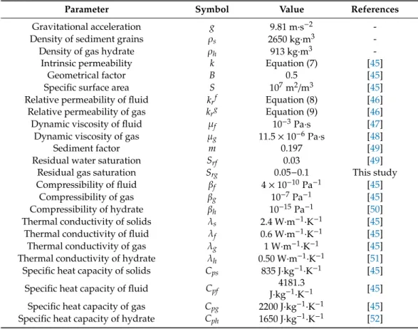
The dynamic viscositiesµf (fluid phase) and µg (gas phase) from Equations (5) and (6) are represented by constant values valid over the investigated pressure and temperature ranges (see Table3).
Table 3.Physical parameters used in numerical simulations (see further description in text).
Parameter Symbol Value References
Gravitational acceleration g 9.81 m·s−2 -
Density of sediment grains ρs 2650 kg·m3 -
Density of gas hydrate ρh 913 kg·m3 -
Intrinsic permeability k Equation (7) [45]
Geometrical factor B 0.5 [45]
Specific surface area S 107m2/m3 [45]
Relative permeability of fluid krf Equation (8) [46]
Relative permeability of gas krg Equation (9) [46]
Dynamic viscosity of fluid µf 10−3Pa·s [47]
Dynamic viscosity of gas µg 11.5×10⁻⁶Pa·s [48]
Sediment factor m 0.197 [49]
Residual water saturation Srf 0.03 [49]
Residual gas saturation Srg 0.05−0.1 This study
Compressibility of fluid βf 4×10⁻¹⁰Pa−1 [45]
Compressibility of gas βg 10−7Pa−1 [45]
Compressibility of hydrate βh 10−15Pa−1 [50]
Thermal conductivity of solids λs 2.4 W·m−1·K−1 [45]
Thermal conductivity of fluid λf 0.6 W·m−1·K−1 [45]
Thermal conductivity of gas λg 1 W·m−1·K−1 [45]
Thermal conductivity of hydrate λh 0.50 W·m−1·K−1 [51]
Specific heat capacity of solids Cps 835 J·kg−1·K−1 [45]
Specific heat capacity of fluid Cpf 4181.3
J·kg−1·K−1 [45]
Specific heat capacity of gas Cpg 2200 J·kg−1·K−1 [45]
Specific heat capacity of hydrate Cph 1650 J·kg−1·K−1 [52]
The intrinsic permeability can be derived from a Kozeny–Carman-type relationship defined according to Equation (7) [45]. ParametersSandBincluded in Equation (7) represent scaling factors valid for various lithologies (see Table3for exact values used in the model). If hydrates are present within the pore space, additional scaling of the intrinsic permeability is required. Thus, effective
porosity and effective tortuosity should be introduced in the Equation (7) asφeff=φ×(1−Sh) and To_eff=1−log (φeff).
k= B·φ
3
To2·S2 (7)
whereB—geometrical factor,To—tortuosity,S—specific surface area.
In a case of a multiphase flow, the relative permeability of fluid (krf) and methane gas (krg) phases are defined as follows [46]:
krf = min Sf−Sr f
1−Sr f−Srg, 1
!!1/2
·
1−
1− min Sf−Sr f
1−Sr f−Srg, 1
!!1/m
m
2
(8) whereSrf—residual saturation of fluid,m—sediment factor.
kgr = 1−min Sf−Sr f 1−Sr f−Srg, 1
!!1/2
·
1−min Sf −Sr f 1−Sr f −Srg, 1
!1/m
2m
(9) whereSrg—residual saturation of gas.
The sediment factor m (Equations (8) and (9)) varies with lithology (see Table3). The residual fluid (Srf) and residual gas (Srg) saturations describe the immobile fraction of each phase (see Table3).
The minimum condition (Min) is introduced to maintain the relative gas permeability (krg) at zero for gas saturations below the residual valueSrg. The exact amount of gas that represents the residual immobile fraction is still under discussion.Srgis believed to have very small values during drainage processes (from 0 to 0.02). Thus, only a small fraction of the upward migrating gas is trapped when gas invaded fluid-filled pores. The hysteresis that occurs during alternating drainage as well as the wetting cycles are not considered in the model since our focus is essentially limited to drainage processes. We found it convenient to useSrg=0.05−0.1 to describe the gas flow reported from naturally occurring gas hydrate provinces (see Table3).
The pore pressure has been calculated according to Equation (10), whereidenotes fluid, free gas, and hydrate phases andjstands for fluid and gas phase only:
X
i
"
φSi
Dρi
Dt
#
=Xj
∇ ·
kkrj
µjρj
∇P+ρj
→
g
−X
i
"
−Siρi 1 (1−φ)
Dφ
Dt +φρiSi ρs
Dρs
Dt
#
(10)
whereSi—saturation of a given phase,ρi—density of a given phase,krj—relative permeability of a given phase,µj—viscosity of a given phase,D—material (substantial) derivative defined as:
D Dt= ∂
∂t+
→
Vs· ∇. (11)
Material derivative (Equation (11)) is commonly used to describe the rate of change of a physical property (e.g., density in Equation (10)) along a solid-flow streamline. The choice of the reference frame used in the model implies that all the material derivatives turns into the normal derivatives due to the fact that the motion of sediment grains (Vsfrom Equation (11)) is accounted for by adjusting the reference frame. The LHS of the Equation (10) accounts for a density change of fluid, gas, and hydrate phase with time. The first term on the RHS accounts for fluid and gas flow. The second term on the RHS describes mechanical sediment compaction and changes in solid density. The values of compressibility factors for fluid, gas, and gas hydrate phases introduced during the Equation (10) derivation (βf,βg, andβh, respectively) are listed in Table3.
Energies2019,12, 3403 9 of 24
Equation (12) shows the general mass balance equation for chemical species dissolved in pore fluids, which is a function of advective and diffusive transport as well as a source term:
∂ φSfC
∂t =∇ ·φSfD∇C
− ∇ · φSfC
→
Vf
+Qf (12)
where C—concentration of chemical species dissolved in pore fluids, D—diffusion coefficient, Qf—source term accounting for bio-chemical reactions occurring in the fluid phase, andt—time.
The rate of molecular diffusion in marine sediments depends on temperature and salinity conditions. Molecular diffusion coefficients (Dm) of chemical species dissolved in pore fluids (CH4, SO4, and DIC) are calculated according to formulations from Boudreau [53]. The effect of tortuosity has been considered by applying the Archie’s law and calculating the diffusion coefficients in sediments (Ds). Diffusive transport of DIC is calculated as a mixture (1:1) of two major DIC species: HCO3and CO2that are widely present at the anoxic, near-neutral pH conditions.
The source termQfin the above mass balance equation accounts for all additional chemical species supply as a result of bio-chemical reaction rates, such as AOM, sulfate reduction, and methanogenesis.
Further description of these processes can be found in the following Section2.1.3.
2.1.3. Source Terms-Bio-Chemical Reactions
The rate of POC degradation greatly influences the amount of gas hydrate formed within the GHSZ [16]. A large amount of globally observed gas hydrate accumulations was formed due to anaerobic decay of a deeply buried organic matter [12,16]. However, only a relatively small fraction of the POC deposited at the seafloor is transported to a certain depth below the bioturbated surface layer of sediments. According to Flogel et al. [54], about 10% of the deposited POC is buried below 10 cm sediment depth at continental margins while only about 1% of POC passes by the bioturbated zone of the first 10 cm of sediments in pelagic deep-ocean environments, which partially explains the lack of gas hydrate deposits in the latter case.
In our model, the rate of organic carbon degradation follows the approach from Middelburg [55]
modified by Wallmann et al. [26], which assumes an age-decreasing reactivity of POC according to the following Equation (13):
RPOC= Kc
C(DIC) +C(CH4) +Kc
·kx·G(POC) (13)
whereRPOCis the rate of organic carbon degradation,C(DIC)—concentration of dissolved inorganic carbon,C(CH4)—concentration of dissolved methane,G(POC)—concentration of solid POC fraction, Kc—Monod inhibition constant,kx—age-dependent kinetic constant.
The age-dependent kinetic constantkxis calculated according to the following expression [55]:
kx=0.16·
a0+ →z
Vs
−0.95
(14)
wherea0—the initial age of organic matter decay (entering the methanogenic zone).
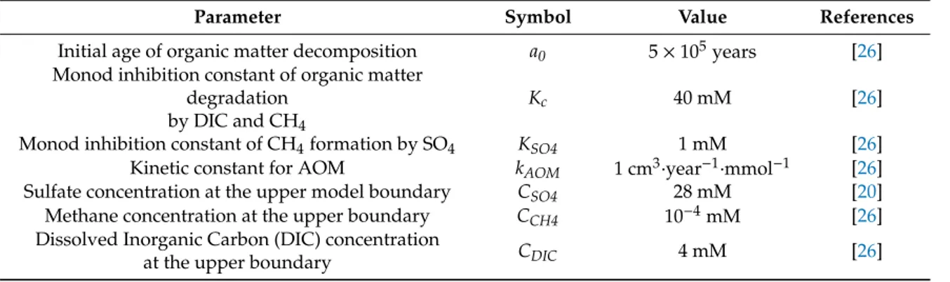
Furthermore, methanogenesis is inhibited in the presence of sulfate such that methane generation occurs only after dissolved sulfate has been depleted by microbial sulfate reduction and AOM [26]. The resulting rates of methane generation and oxidation are applied as source termQin the mass balance equation for methane (Equation (11)) to quantify the supply ofCH4into the system as a result of above microbial reactions. The full compilation of modeling parameters considering POC degradation and AOM processes at the Blake Ridge Site 997 is presented in Table4.
Table 4. Geochemical parameters used in numerical modeling scenarios for Site 997 (see further description in text).
Parameter Symbol Value References
Initial age of organic matter decomposition a0 5×10⁵years [26]
Monod inhibition constant of organic matter degradation
by DIC and CH4
Kc 40 mM [26]
Monod inhibition constant of CH4formation by SO4 KSO4 1 mM [26]
Kinetic constant for AOM kAOM 1 cm3·year−1·mmol−1 [26]
Sulfate concentration at the upper model boundary CSO4 28 mM [20]
Methane concentration at the upper boundary CCH4 10−4mM [26]
Dissolved Inorganic Carbon (DIC) concentration
at the upper boundary CDIC 4 mM [26]
In the model, density of pore fluids occupying the pore space of sediments depends on temperature, pressure, salt content, and dissolved methane. To calculate the density of a H2O–NaCl mixture, we have used a numerical toolbox for Matlab [56]. Density of a H2O–NaCl–CH4mixture was calculated from the equation-of-state derived by Duan et al. [57]. Methane gas density, methane gas solubility, and gas hydrate solubility are calculated as time-dependent variables according to the equations from Tishchenko et al. [44] and Duan et al. [57], which include the effect of salinity.
2.1.4. Temperature
The temperature field is calculated according to Equation (15) assuming a constant heat flux at the bottom of a modeling domain (zmax(t)) and a fixed temperature value at the sea-surface (z=0):
ρCp
bulk
∂T
∂t =−ρCp
bulk
→
Vs· ∇T−ρfCpf
→
Uf· ∇T−ρgCpg
→
Ug· ∇T+∇ ·(λbulk∇T) +Q (15) whereT—temperature,(ρCp)bulk—volumetric heat capacity,Cpf—heat capacity of fluid phase,Cpg—heat capacity of gas phase,λbulk—bulk thermal conductivity,Q—latent heat from melting hydrates.
Bulk volumetric heat capacity accounts for all phases present in the model according to their saturations, which contribute to the total energy balance:
ρCp
bulk= (1−φ)ρsCps+φSfρfCpf +φSgρgCpg+φShρhCph (16) whereCph—heat capacity of hydrate phase.
According to Deming and Chapman [58], bulk thermal conductivity can be expressed as:
λbulk=λs(1−φ)λfφ (17) whereλs—thermal conductivity of solid phase,λf—thermal conductivity of fluid phase.
However, in the four-phase system, we have to include another two terms accounting for hydrate and free gas components [59]:
λbulk=λs(1−φ)λfSfφλgSgφλhShφ (18) whereλg—thermal conductivity of gas phase,λh—thermal conductivity of hydrate phase.
According to Waite et al. [59], in porous (>30%) sediments filled in by at least 10% hydrates, gas hydrate contribution to the bulk thermal conductivity increases significantly. We found the number of 0.65 W·m−1·K−1accounting for the thermal conductivity of gas hydrate convenient and used this constant value in our simulations. Latent heat from gas hydrate dissociation (termQin Equation (14)) has a constant value of 450 kJ kg−1(equivalent to 53.8 kJ mol−1) as it was previously reported [25].
Energies2019,12, 3403 11 of 24
2.2. Numerical Model 2.2.1. Reference Frame
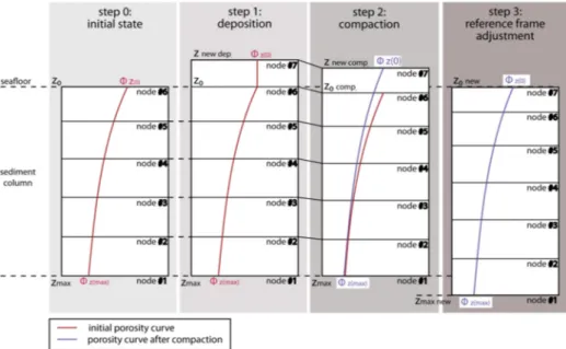
We use a reference frame that is attached to the seafloor. During each time step, sediments are deposited according to a prescribed rate. Subsequently, compaction occurs and the seafloor is adjusted back to zero by shifting the entire sediment package downwards. This approach allows for the variable deposition of different rock types through time, and a schematic visualization of the reference frame concept is shown in Figure2.
Energies 2019, 12, 3403 11 of 24
2.2. Numerical Model
2.2.1. Reference Frame
We use a reference frame that is attached to the seafloor. During each time step, sediments are deposited according to a prescribed rate. Subsequently, compaction occurs and the seafloor is adjusted back to zero by shifting the entire sediment package downwards. This approach allows for the variable deposition of different rock types through time, and a schematic visualization of the reference frame concept is shown in Figure 2.
Figure 2. Schematic illustration of the reference frame concept used in the model previously validated by Schmidt et al. [60]. Starting from the left: Step 0 represents the initial state of modeled sedimentary column extending from the seafloor (z0) to the maximum sediment depth (zmax) with an initial porosity curve (red line) ranging from high seafloor porosity value (ɸz(0)) up to low maximum sediment depth value (ɸz(max)) containing an initial number of nodes in the z-direction. In step 1, a new sedimentary layer, represented by the node #7, has been deposited on top of the existing column. The top of the new layer has been marked by the znewdep. symbol and porosity of the new layer remains constant with depth. Step 2 depicts a compaction process of all deposited layers according to their lithological properties (in the drawing assumed to be homogeneous for simplicity) and a new porosity curve (violet line) as a result of this process. Finally, step 3 shows a vertical adjustment of the reference frame to match the upper boundary of sedimentary column with the seafloor coordinates z0 and a new porosity curve (violet line). Note that porosity curves, including initial (seafloor) porosity values, are only symbolic and do not represent the real compaction properties of the Blake Ridge sediments.
Sediment compaction occurs according to a depth-dependent parametrization of porosity (Equation (19)).
( )
z( )
0exp ( c z
0)
φ = φ ⋅ ⋅
(19)where ϕ(z)—porosity change with depth, ϕ(0)—initial porosity on top of a sediment layer, z—depth, c0—the compaction length scale of a given lithology.
As sediment consolidation drives fluid flow and thereby reactive-transport within the sediment column, variations in sediment type and associated compaction behavior can potentially have a significant influence on pore fluid chemistry—an effect that our model allows us to investigate.
In general, methane supply to the GHSZ can occur via three distinct processes: In-situ CH4
formation within stability zone, advective fluid transport from below, or by rising free gas. In the simple case of in-situ methane generation, no flux boundary conditions are prescribed at the bottom of the modeling column. Fluids expelled by sediment compaction move upwards with respect to the
Figure 2.Schematic illustration of the reference frame concept used in the model previously validated by Schmidt et al. [60]. Starting from the left: Step 0 represents the initial state of modeled sedimentary column extending from the seafloor (z0) to the maximum sediment depth (zmax) with an initial porosity curve (red line) ranging from high seafloor porosity value (Φz(0)) up to low maximum sediment depth value (Φz(max)) containing an initial number of nodes in the z-direction. In step 1, a new sedimentary layer, represented by the node #7, has been deposited on top of the existing column. The top of the new layer has been marked by the znew dep.symbol and porosity of the new layer remains constant with depth. Step 2 depicts a compaction process of all deposited layers according to their lithological properties (in the drawing assumed to be homogeneous for simplicity) and a new porosity curve (violet line) as a result of this process. Finally, step 3 shows a vertical adjustment of the reference frame to match the upper boundary of sedimentary column with the seafloor coordinates z0and a new porosity curve (violet line). Note that porosity curves, including initial (seafloor) porosity values, are only symbolic and do not represent the real compaction properties of the Blake Ridge sediments.
Sediment compaction occurs according to a depth-dependent parametrization of porosity (Equation (19)).
φ(z)=φ(0)·exp(c0·z) (19) whereφ(z)—porosity change with depth,φ(0)—initial porosity on top of a sediment layer,z—depth, c0—the compaction length scale of a given lithology.
As sediment consolidation drives fluid flow and thereby reactive-transport within the sediment column, variations in sediment type and associated compaction behavior can potentially have a significant influence on pore fluid chemistry—an effect that our model allows us to investigate.
In general, methane supply to the GHSZ can occur via three distinct processes: In-situ CH4
formation within stability zone, advective fluid transport from below, or by rising free gas. In the simple case of in-situ methane generation, no flux boundary conditions are prescribed at the bottom of
the modeling column. Fluids expelled by sediment compaction move upwards with respect to the sediment grains. However, due to the deposition of new sedimentary layers, expelled pore fluids never reach the seafloor. In the case of a prescribed fluid flux at the base, two additional scenarios of fluid migration are possible: (1) Either the rate of fluid influx is sufficiently high to overcome the burial velocity so that fluid venting occurs at the seafloor, or (2) burial continues to dominate and the increase in upward fluid flux continues to be insufficient for seafloor venting to occur.
2.2.2. Initial and Boundary Conditions
At the beginning of each run, constant concentrations of dissolved CH4, SO4, and DIC are prescribed at the top of the modeling column according to the values given in Table4. Additionally, sulfate concentration profile at the beginning of each model run is initialized to decrease exponentially with depth. Concentration of POC (wt.%) at the top of sediment column is set to 1.6 wt.% (see Table1) and stays constant (Scenarios 1-2, and 4) or decreases with time (Scenarios 3 and 5). Salinity of pore fluids is assumed to be constant (see Table1). To initialize the P-T conditions, we use a hydrostatic pressure that accounts for NaCl and CH4-dependent fluid density, constant bottom water temperature, and a steady-state geotherm to match the local measurements (see Table1).
2.2.3. Solution Algorithm
Each computational step starts with the deposition of a new sedimentary layer according to the sedimentation rate and the time-step size (dt). Next, compaction is accounted for and the top of the modeling domain is adjusted accordingly. The change in porosity is driving pore pressure, which is calculated using a finite elements (FE) scheme. Darcy velocity calculations for fluid and gas phase are based on the outcome of the pressure solver and relative permeability computation. At this stage, the Courant number is calculated, which limits the time-step in case of a Darcy flow exceeding the volume of one modeling cell. If the time-step needs to be reduced, the solution algorithm starts from the beginning, which implies that the pore pressure is computed again with a reduceddt. The temperature solver calculates the temperature profile for the entire sedimentary column. According to the temperature profile, diffusion coefficients for the dissolved chemical species are updated. Advection and diffusion calculations are split and solved separately for each phase using a finite volumes (FV) numerical approach. The last part of the numerical procedure contains computation of all bio-chemical reactions occurring in the system. Equation-of-state (EOS) for brine-gas–gas hydrate system is applied at the end to account for new saturations, densities, and volume changes of each phase. The model has been entirely implemented in Matlab v.2018.
3. Results and Discussion
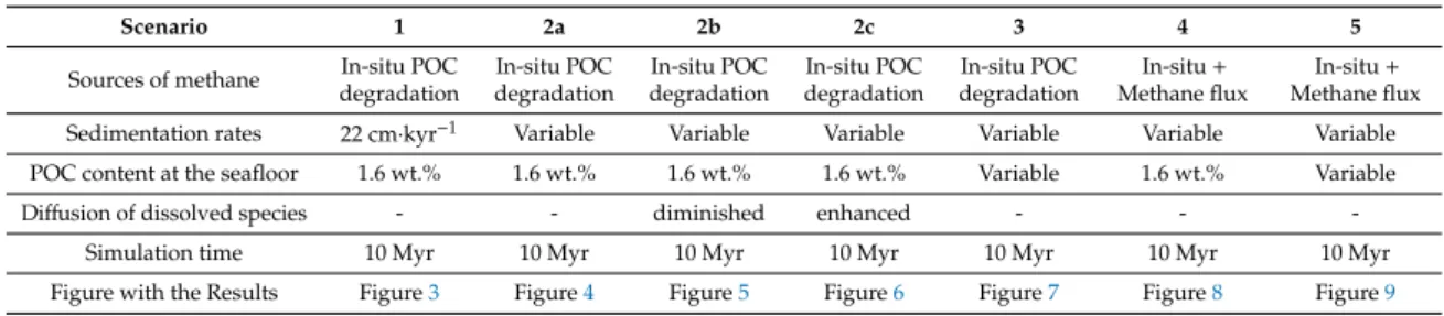
To investigate gas hydrate formation from a single in-situ methane source as well as the possible impact of an upward fluid flux at the Blake Ridge Site, we have explored seven numerical modeling scenarios listed in Table5. Detailed descriptions of each modeling scenario as well as the results are presented below.
Table 5.Summary of modeling scenarios presented in the study.
Scenario 1 2a 2b 2c 3 4 5
Sources of methane In-situ POC degradation
In-situ POC degradation
In-situ POC degradation
In-situ POC degradation
In-situ POC degradation
In-situ+ Methane flux
In-situ+ Methane flux Sedimentation rates 22 cm·kyr−1 Variable Variable Variable Variable Variable Variable POC content at the seafloor 1.6 wt.% 1.6 wt.% 1.6 wt.% 1.6 wt.% Variable 1.6 wt.% Variable
Diffusion of dissolved species - - diminished enhanced - - -
Simulation time 10 Myr 10 Myr 10 Myr 10 Myr 10 Myr 10 Myr 10 Myr
Figure with the Results Figure3 Figure4 Figure5 Figure6 Figure7 Figure8 Figure9
Energies2019,12, 3403 13 of 24
Energies 2019, 12, 3403 13 of 24
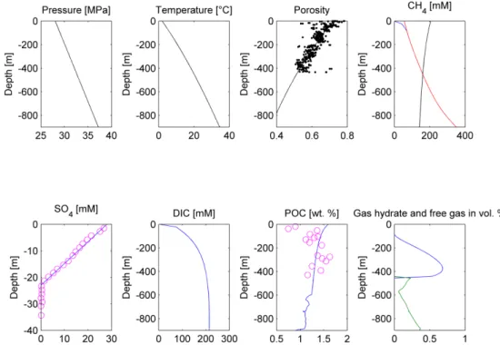
Figure 3. Modeling results for the Scenario 1. Upper panel, from the left: Pressure, temperature, porosity, and dissolved CH4 concentration plots. Porosity measurements [20] are depicted as black dots, the modeling solution is represented by the black line. On the CH4 concentration plot, red line depicts the phase boundary between gas hydrate and dissolved methane, black line represents the phase boundary between free gas and dissolved methane, and blue line states dissolved methane concentration. Gas hydrate and/or free gas formation occurs wherever dissolved methane concentration exceeds one of the solubility curves. Lower panel, from the left: SO4, dissolved inorganic carbon (DIC), POC, and gas hydrate/free gas concentration plots (in blue and green, respectively). On the SO4 and POC concentration plot, measured values are presented as pink circles [20], whereas model predictions are shown as the blue lines.
Figure 4. Modeling results of the Scenario 2a. Upper panel, from the left: Pressure, temperature, porosity, and dissolved CH4 concentration plots. Porosity measurements [20] are depicted as black dots, the modeling solution is represented by the black line. On the CH4 concentration plot, red line Figure 3. Modeling results for the Scenario 1. Upper panel, from the left: Pressure, temperature, porosity, and dissolved CH4concentration plots. Porosity measurements [20] are depicted as black dots, the modeling solution is represented by the black line. On the CH4concentration plot, red line depicts the phase boundary between gas hydrate and dissolved methane, black line represents the phase boundary between free gas and dissolved methane, and blue line states dissolved methane concentration. Gas hydrate and/or free gas formation occurs wherever dissolved methane concentration exceeds one of the solubility curves. Lower panel, from the left: SO4, dissolved inorganic carbon (DIC), POC, and gas hydrate/free gas concentration plots (in blue and green, respectively). On the SO4and POC concentration plot, measured values are presented as pink circles [20], whereas model predictions are shown as the blue lines.
Energies 2019, 12, 3403 13 of 24
Figure 3. Modeling results for the Scenario 1. Upper panel, from the left: Pressure, temperature, porosity, and dissolved CH4 concentration plots. Porosity measurements [20] are depicted as black dots, the modeling solution is represented by the black line. On the CH4 concentration plot, red line depicts the phase boundary between gas hydrate and dissolved methane, black line represents the phase boundary between free gas and dissolved methane, and blue line states dissolved methane concentration. Gas hydrate and/or free gas formation occurs wherever dissolved methane concentration exceeds one of the solubility curves. Lower panel, from the left: SO4, dissolved inorganic carbon (DIC), POC, and gas hydrate/free gas concentration plots (in blue and green, respectively). On the SO4 and POC concentration plot, measured values are presented as pink circles [20], whereas model predictions are shown as the blue lines.
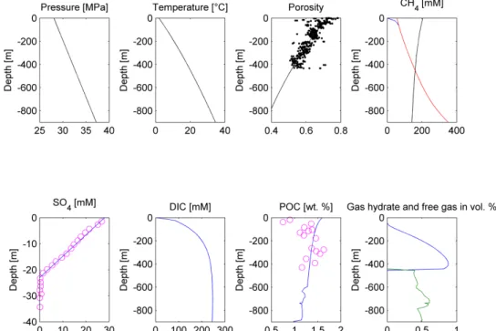
Figure 4. Modeling results of the Scenario 2a. Upper panel, from the left: Pressure, temperature, porosity, and dissolved CH4 concentration plots. Porosity measurements [20] are depicted as black dots, the modeling solution is represented by the black line. On the CH4 concentration plot, red line Figure 4.Modeling results of the Scenario 2a. Upper panel, from the left: Pressure, temperature, porosity, and dissolved CH4concentration plots. Porosity measurements [20] are depicted as dots, black the
modeling solution is represented by the black line. On the CH4concentration plot, red line depicts the phase boundary between gas hydrate and dissolved methane, black line represents the phase boundary between free gas and dissolved methane, blue line states dissolved methane concentration.
Gas hydrate and/or free gas formation occurs wherever dissolved methane concentration exceeds one of the solubility curves. Lower panel, from the left: SO4, DIC, POC, and gas hydrate/free gas concentration plots (in blue and green, respectively). On the SO4and POC concentration plot, measured values are presented as pink circles [20], whereas model predictions are shown as the blue lines.
Energies 2019, 12, 3403 14 of 24
depicts the phase boundary between gas hydrate and dissolved methane, black line represents the phase boundary between free gas and dissolved methane, blue line states dissolved methane concentration. Gas hydrate and/or free gas formation occurs wherever dissolved methane concentration exceeds one of the solubility curves. Lower panel, from the left: SO4, DIC, POC, and gas hydrate/free gas concentration plots (in blue and green, respectively). On the SO4 and POC concentration plot, measured values are presented as pink circles [20], whereas model predictions are shown as the blue lines.
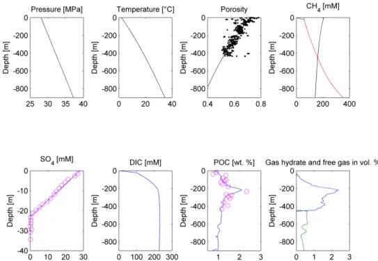
Figure 5. Modeling results of the Scenario 2b. Upper panel, from the left: Pressure, temperature, porosity, and dissolved CH4 concentration plots. Porosity measurements [20] are depicted as black dots, the modeling solution is represented by the black line. On the CH4 concentration plot, red line depicts the phase boundary between gas hydrate and dissolved methane, black line represents the phase boundary between free gas and dissolved methane, blue line states dissolved methane concentration. Gas hydrate and/or free gas formation occurs wherever dissolved methane concentration exceeds one of the solubility curves. Lower panel, from the left: SO4, DIC, POC, and gas hydrate/free gas concentration plots (in blue and green, respectively). On the SO4 and POC concentration plot, measured values are presented as pink circles [20], whereas model predictions are shown as the blue lines.
Figure 5. Modeling results of the Scenario 2b. Upper panel, from the left: Pressure, temperature, porosity, and dissolved CH4concentration plots. Porosity measurements [20] are depicted as black dots, the modeling solution is represented by the black line. On the CH4concentration plot, red line depicts the phase boundary between gas hydrate and dissolved methane, black line represents the phase boundary between free gas and dissolved methane, blue line states dissolved methane concentration.
Gas hydrate and/or free gas formation occurs wherever dissolved methane concentration exceeds one of the solubility curves. Lower panel, from the left: SO4, DIC, POC, and gas hydrate/free gas concentration plots (in blue and green, respectively). On the SO4and POC concentration plot, measured values are presented as pink circles [20], whereas model predictions are shown as the blue lines.
Energies2019,12, 3403 15 of 24
Energies 2019, 12, 3403 15 of 24
Figure 6. Modeling results of the Scenario 2c. Upper panel, from the left: Pressure, temperature, porosity, and dissolved CH4 concentration plots. Porosity measurements [20] are depicted as black dots, the modeling solution is represented by the black line. On the CH4 concentration plot, red line depicts the phase boundary between gas hydrate and dissolved methane, black line represents the phase boundary between free gas and dissolved methane, blue line states dissolved methane concentration. Gas hydrate and/or free gas formation occurs wherever dissolved methane concentration exceeds one of the solubility curves. Lower panel, from the left: SO4, DIC, POC, and gas hydrate/free gas concentration plots (in blue and green, respectively). On the SO4 and POC concentration plot, measured values are presented as pink circles [20], whereas model predictions are shown as the blue lines.
Figure 7. Modeling results of the Scenario 3. Upper panel, from the left: Pressure, temperature, porosity, and dissolved CH4 concentration plots. Porosity measurements [20] are depicted as black dots, the modeling solution is represented by the black line. On the CH4 concentration plot, red line depicts the phase boundary between gas hydrate and dissolved methane, black line represents the phase boundary between free gas and dissolved methane, blue line states dissolved methane
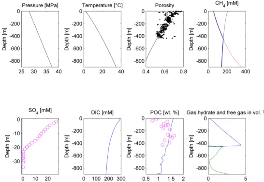
Figure 6. Modeling results of the Scenario 2c. Upper panel, from the left: Pressure, temperature, porosity, and dissolved CH4concentration plots. Porosity measurements [20] are depicted as black dots, the modeling solution is represented by the black line. On the CH4concentration plot, red line depicts the phase boundary between gas hydrate and dissolved methane, black line represents the phase boundary between free gas and dissolved methane, blue line states dissolved methane concentration.
Gas hydrate and/or free gas formation occurs wherever dissolved methane concentration exceeds one of the solubility curves. Lower panel, from the left: SO4, DIC, POC, and gas hydrate/free gas concentration plots (in blue and green, respectively). On the SO4and POC concentration plot, measured values are presented as pink circles [20], whereas model predictions are shown as the blue lines.
Energies 2019, 12, 3403 15 of 24
Figure 6. Modeling results of the Scenario 2c. Upper panel, from the left: Pressure, temperature, porosity, and dissolved CH4 concentration plots. Porosity measurements [20] are depicted as black dots, the modeling solution is represented by the black line. On the CH4 concentration plot, red line depicts the phase boundary between gas hydrate and dissolved methane, black line represents the phase boundary between free gas and dissolved methane, blue line states dissolved methane concentration. Gas hydrate and/or free gas formation occurs wherever dissolved methane concentration exceeds one of the solubility curves. Lower panel, from the left: SO4, DIC, POC, and gas hydrate/free gas concentration plots (in blue and green, respectively). On the SO4 and POC concentration plot, measured values are presented as pink circles [20], whereas model predictions are shown as the blue lines.
Figure 7. Modeling results of the Scenario 3. Upper panel, from the left: Pressure, temperature, porosity, and dissolved CH4 concentration plots. Porosity measurements [20] are depicted as black dots, the modeling solution is represented by the black line. On the CH4 concentration plot, red line depicts the phase boundary between gas hydrate and dissolved methane, black line represents the phase boundary between free gas and dissolved methane, blue line states dissolved methane Figure 7.Modeling results of the Scenario 3. Upper panel, from the left: Pressure, temperature, porosity, and dissolved CH4concentration plots. Porosity measurements [20] are depicted as black dots, the modeling solution is represented by the black line. On the CH4concentration plot, red line depicts the
![Table 2. Rates of sediment accumulation at Blake Ridge Site 997 after Ikeda et al. [37].](https://thumb-eu.123doks.com/thumbv2/1library_info/5295233.1677289/4.892.128.762.318.584/table-rates-sediment-accumulation-blake-ridge-site-ikeda.webp)