A fast polygon inflation algorithm to compute the area of feasible solutions for three-component systems. I: Concepts and applications.
Mathias Sawalla, Christoph Kubisb, Detlef Selentb, Armin B¨ornerb, Klaus Neymeyra
aUniversit¨at Rostock, Institut f¨ur Mathematik, Ulmenstrasse 69, 18057 Rostock, Germany
bLeibniz-Institut f¨ur Katalyse, Albert-Einstein-Strasse 29a, 18059 Rostock
Abstract
The multicomponent factorization of multivariate data often results in non-unique solutions. The so-called rotational ambiguity paraphrases the existence of multiple solutions which can be represented by the area of feasible solutions (AFS). The AFS is a bounded set which may consist of isolated subsets. The numerical computation of the AFS is well understood for two-component systems and is an expensive numerical process for three-component systems. In this paper a new fast and accurate algorithm is suggested which is based on the inflation of polygons. Starting with an initial triangle located in a topologically-connected subset of the AFS, an automatic extrusion algorithm is used to form a sequence of growing polygons which approximate the AFS from the interior. The polygon inflation algorithm can be generalized to systems with more than three components. The efficiency of this algorithm is demonstrated for a model problem including noise and a multi-component chemical reaction system. Further, the method is compared with the recent triangle-boundary-enclosing scheme of Golshan, Abdollahi and Maeder (Anal. Chem. 2011, 83, 836–
841).
Key words: factor analysis, pure component decomposition, nonnegative matrix factorization, spectral recovery, band boundaries of feasible solutions, polygon inflation.
1. Introduction
The resolution of multicomponent mixtures is a chal- lenge in analytic chemistry which uses for its solu- tion mathematical tools of nonnegative matrix factor- izations. We consider the inverse problem to compute from a spectral data matrix on a time×frequency grid an approximate factorization into a concentration and an absorptivity matrix. These matrices represent the con- centration profiles in time and the absorption spectra of the pure components underlying the chemical reaction system. A serious obstacle of a pure component de- composition procedure is the fact that in nearly all cases a continuum of feasible solutions exists. This fact is well-known from the analysis of relatively simple two- component systems published by Lawton and Sylvestre in 1971 [19]. For three-component systems Borgen and Kowalski [5] provided valuable techniques on the pure component recovery which were extended and deep- ened by Rajk `o and Istv´an [26] and also by Golshan, Ab- dollahi and Maeder [10, 11]. Closely related to this is the computation of minimal and maximal band bound- aries by Tauler [29]. For general literature on the pure
component decomposition see Malinowski [21], Hamil- ton and Gemperline [14] and Maeder and Neuhold [20].
In this paper the focus is on the numerical approx- imation of the area of feasible solutions (AFS) for three-component systems. The approach by Borgen and Kowalski [5] allows to represents the AFS by a bounded set in a 2D plane. For a three-component system the AFS is expected to consist of at most three separated subsets. Our work is also inspired by the recent work of Golshan, Abdollahi and Maeder [10] in which the boundary of the AFS is covered by a chain of equilat- eral triangles.
1.1. The new polygon inflation algorithm
Our idea to approximate the AFS of a three- component system is to inflate an initial triangle in the interior of a topologically-connected subset by an adap- tive algorithm. The inflation algorithm subdivides the edges of the polygon recursively and adds new vertices which are located on the boundary of the AFS. A local error estimation is used to control the polygon refine- ment.
... February 14, 2013
−1 0 1 0
0.5 1 1.5 2 2.5
N=3
−1 0 1
0 0.5 1 1.5 2 2.5
N=4
−1 0 1
0 0.5 1 1.5 2 2.5
N=12
−1 0 1
0 0.5 1 1.5 2 2.5
N=125
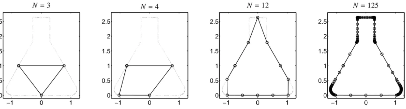
Figure 1: Approximation of the boundary of an Erlenmeyer flask. The initial triangle (left figure) and refined polygons with N=4,12,125 vertices are shown. The vertices are computed in an adaptive algorithm in a way that the approximation error is minimized. See Sections 3.4 and 3.5 for the explanation of the parametersεbandδ: Withεb=δ=10−3one gets 125 final vertices, forεb =δ=10−4a number of 309 vertices and for εb=δ=10−5a number of 781 vertices.
The polygon inflation is illustrated in Figure 1 where the shape of an Erlenmeyer flask, for demonstration pur- poses, is approximated. A characteristic feature of the algorithm is that it requires only few vertices to approx- imate straight segments of the boundary. For curved re- gions the resolution is increased automatically within the adaptive process. The idea of a polygon inflation can be generalized to higher dimensions. A 3D poly- hedral construction can be used to treat four-component systems and so on.
1.2. Organization of the paper
Section 2 introduces the Borgen-Kowalski approach for representing the AFS by means of a planar plot for three-component systems. Further, the triangle- boundary-enclosing algorithm from [10] is explained.
In Section 3 the new polygon inflation algorithm is pre- sented and its adaptivity and efficiency are discussed.
Numerical examples are presented in Sections 4 and 5 where the AFS is computed for the Rhodium-catalyzed hydroformylation. The precision of the algorithm is an- alyzed under variation of the control parameters and the algorithm is compared with established methods.
2. On the representation of feasible solutions 2.1. The spectral recovery problem
Let D∈Rk×nbe the spectral data matrix which con- tains in its rows k spectra (taken at k times from a chem- ical reaction system) and where each spectrum contains absorption values at n frequencies. If the reaction sys- tem contains s active species with s ≤ min(k,n), then the concentration matrix C ∈ Rk×s contains column- wise the concentration profiles of these species. The absorptivity matrix A∈ Rs×nholds row-wise the spec- tra of these s species. If nonlinearities and noise are
ignored, then the Lambert-Beer law expresses a linear dependence between D, C and A in the form
D=CA.
The problem of a multivariate curve resolution tech- nique is to find for a given matrix D the correct non- negative matrix factors C and A, see [14, 21]. This is a so-called inverse problem which is ill-posed in the sense that a continuum of possible solutions exists [20]. The following options are available:
1. One can try to recover the desired pure component decomposition by using regularization techniques and/or kinetic models [2, 7, 9, 13, 16, 24, 27].
However, these regularization techniques entail the risk that improper solutions are picked out.
2. In appropriate cases the non-uniqueness can be re- duced by a local rank analysis together with an ap- plication of the theorems of Manne [22]. Further, partial knowledge of spectra, e.g. of the reactants, or the knowledge of certain concentration profiles allows to apply the complementarity and coupling theorems from [28]. These and other arguments can result in a unique decomposition or at least in some unique factors.
3. If no adscititious information on the reaction sys- tem is to be included in the factor analysis, then a computation of the set of all possible solutions ap- pears to be appropriate. See [1, 8, 10, 19, 29] for the AFS for two- and three-component systems.
Here we follow this third and most general approach and aim at a computation of the AFS. Moreover, the AFS can be considered as an own object of research. Numer- ical methods for its computation appear to be desirable.
2
2.2. A low-dimensional representation of the AFS The starting point for the computation of the AFS is a singular value decomposition (SVD) of the spectral data matrix D ∈ Rk×n. Its SVD reads D =UΣVT with or- thogonal matrices U,V and the diagonal matrixΣwhich contains the singular valuesσi on its diagonal. If D is a rank-s matrix, then it holds that D=UΣVT =U ˜˜ΣV˜T with ˜U=U(:,1 : s)∈ Rk×s, ˜Σ = Σ(1 : s,1 : s)∈Rs×s and ˜V=V(:,1 : s)∈Rn×s.
The so-called abstract factors ˜U ˜Σand ˜VTare usually poor approximations of the matrices C and A. A proper regular transformation by T ∈ Rs×s allows to solve the reconstruction problem according to
C=U ˜˜ΣT−1, A=T ˜VT. (1) Any pair of nonnegative matrices ˜U ˜ΣT−1 and T ˜VT is called a feasible solution. A feasible solution guaran- tees a correct reconstruction since D=( ˜U ˜ΣT−1)(T ˜VT).
However, these factors may have no chemical meaning.
For a two-component system Lawton and Sylvestre [19] have represented the range of feasible solutions.
For a three-component system the situation is more complicated but the purpose is still the same. All reg- ular matrices T are to be found so that C and A in (1) are nonnegative matrices. The coefficients of T are the key for a low-dimensional representation of the AFS, see the seminal work of Borgen and Kowalski [5], the important contributions [4, 8, 26, 25] as well as the re- cent paper [10]. The approach is explained next.
The Perron-Frobenius theory [23] guarantees that the first singular vector V(:,1) of V can be assumed to be a component-wise nonnegative vector; possibly a multi- plication with−1 is to be applied to give a component- wise non-positive vector the desired orientation. With (1) the ith pure component spectrum A(i,:), i =1,2,3, reads
A(i,:)=ti1V(:,1)T+ti2V(:,2)T+ti3V(:,3)T. (2) Since V(:,1) , 0 these spectra can be scaled so that ti1 = 1 for i = 1,2,3. Then T has still six degrees of freedom namely ti2and ti3with i=1,2,3. The problem is forced to two dimensions by looking only for those α:=t12andβ:=t13so that
T =
1 α β
1 s11 s12
1 s21 s22
. (3) for proper s11,s12,s21and s22 results in a feasible solu- tion.
A point (α, β)∈R2is called valid if and only if there exists at least one regular matrix
S = s11 s12
s21 s22
!
∈R2×2, (4) so that T is invertible and both A = T ˜VT and C = U ˜˜ΣT−1 are nonnegative matrices. Hence the AFS can be expressed as the set
M=n
(α, β)∈R2: rank(T )=3, C,A≥0o
. (5)
Under some mild assumptions the setMis bounded.
The rows of S andα, βare coupled in the following sense: If (α, β) ∈ M, then the rows S (i,:), i = 1,2, of S are also contained in M. The reason is that an orthogonal permutation matrix P∈R3×3can be inserted in the admissible factorization
D=CA=U ˜˜ΣT−1T ˜VT =( ˜U ˜ΣT| {z }−1PT
(PT )−1
) (PT ˜VT).
The permutation of the rows of T is accompanied with the associated permutation of the columns of T−1 and the nonnegativity of the factors is preserved. Further PT and T−1PT =(PT )−1are a pair of transformation matri- ces with permuted rows/columns in a way that (si1,si2) can substitute (α, β) and vice versa.
2.3. The triangle-boundary-enclosing approach of Gol- shan, Abdollahi and Maeder
In 2011 Golshan, Abdollahi and Maeder [10] intro- duced a new approach for the numerical approximation of the boundary of the AFS. This technique is based on an inclusion of the boundary by small equilateral trian- gles. The algorithm constructs in an initialization phase a first triangle which has at least one vertex in the inte- rior ofMand has also at least one vertex which is not in M. Thus the boundary of the AFS has a nonempty inter- section withM. Next this triangle is reflected along one of its edges in a way that the new triangle has once again a vertex in and a vertex not in M. This procedure is continued until the band of triangles includes the entire boundary of a connected subset of the AFS, see Figure 2. The accuracy of this triangle-boundary-enclosing ap- proach depends on the edge length of the triangles. For smaller triangles the accuracy of the boundary approxi- mation increases together with total number of triangles which are used to cover the boundary.
3. The polygon inflation algorithm
The geometric idea of the polygon inflation algorithm is introduced in Section 1.1. Next we describe the algo- rithm and its mathematical fundamentals.
3
Figure 2: Enclosure of a boundary segment by a chain of equilateral triangles.
3.1. The target function for approximating the AFS For the computation of the AFS a procedure to clas- sify points (α, β) ∈ R2 as valid, if (α, β) ∈ M, or as non-valid in the other case. A procedure for this classi- fication is developed next. Letε≥0 be a small nonneg- ative real number. Then−εis used as a lower bound for the acceptable relative negativeness of the factors C and A in the following way
minjCji
maxj|Cji| ≥ −ε, minjAi j
maxj|Ai j| ≥ −ε, i=1,2,3. (6) The acceptance of small negative components of C and A allows to stabilize the computational process in the case of noisy data.
Let f be a target function which depends on the six degrees of freedom beingα,βand S ∈R2×2, see (3) and (4), so that
f :R×R×R2×2→R with
f (α, β,S )= X3
i=1
Xk
j=1
min(0, Cji
kC(:,i)k∞
+ε)2
+ X3
i=1
Xn
j=1
min(0, Ai j kA(i,:)k∞
+ε)2 +kI3−T T+k2F.
(7)
Therein C and A are formed according to (1), I3 ∈R3×3 is the 3×3 identity matrix,k · k∞is the maximum vector norm andk · kF is the Frobenius matrix norm [12]. Fur- ther T+is the pseudo-inverse of T . The last summand kI3−T T+k2F equals zero if T is an invertible matrix and is positive if T is singular; therefore f =0 guarantees a regular T . The function f is used to form F as follows
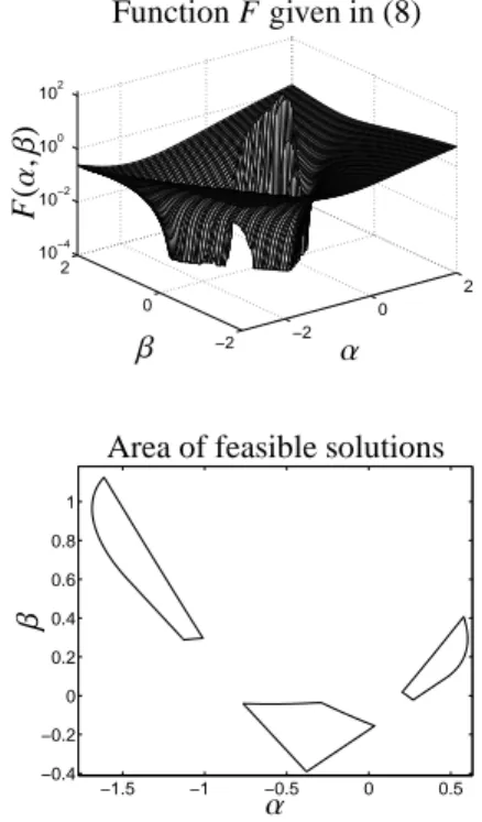
F :R2 →R, F(α, β)= min
S∈R2×2 f (α, β,S ). (8)
−2 0
2
−2 0 2 10−4 10−2 100 102
β α
F(α,β)
Function F given in (8)
−1.5 −1 −0.5 0 0.5
−0.4
−0.2 0 0.2 0.4 0.6 0.8 1
α
β
Area of feasible solutions
Figure 3: The AFS for the model problem from Section 4. Top:
F(α, β) on (α, β)∈[−2,2]×[−2,2]. Bottom: The AFS withεb=10−4, see (11).
Computationally a point (α, β) is considered as valid if and only if F(α, β)≤εtolwithεtol=10−10. Hence,
M=n
(α, β)∈R2: F(α, β)≤εtol
o. (9) Figure 3 illustrates F for the model problem which is presented in Section 4 on the domain (α, β)∈[−2,2]× [−2,2].
The evaluation of F requires the solution of a least- squares problem within 4 parameters and with 3(k + n+3) variables. Our function F given in (8) is some- what different from the pure sum of squares ssq = kD−C+A+k2F as used in [1, 10, 30]; therein C+and A+
are derived from C and A by removing any negative en- tries. However, we prefer to use (8) for the reason of its numerical stability and as (8) requires a minimization of a sum of onlyO(k+n) squares. In contrast to this, the minimization of ssq includes the much larger number ofO(k·n) summands of squares. Here, the number of components is fixed to s=3. If the approach is gener- alized to larger s, then the computational costs increase linearly in s.
3.2. Orientation of the AFS
The orientation of the AFS M depends on the ori- entation of the singular vectors. The orientation of a 4
singular vector means that the sign of a singular vector is not uniquely determined in the sense that the simul- taneous multiplication of the ith left singular vector and the ith right singular vector with−1 does not change the product UΣVT. However, the orientation of the first left singular vector and the first right singular vector can be fixed in advance by the Perron-Frobenius theory as these two vectors are sign-constant and can therefore be assumed in a component-wise nonnegative form. In other words the SVD UΣVT with U ∈Rk×3, V ∈ Rn×3 is equivalent to the SVD ˆUΣVˆT with
U(:,ˆ 1 : 3)=U(:,1 : 3)·diag(1,p1,p2), V(:,ˆ 1 : 3)=V(:,1 : 3)·diag(1,p1,p2)
and p1,p2∈ {−1,1}. The signs of piare associated with a reflection of the AFS along theα- or theβ-axes.
3.3. Initialization: Generation of a first triangle Here we refer to the typical case that the AFS consists of three separated subsets. However, the algorithm can also be applied to all other cases. Further the AFS is assumed to be a bounded set; we plan to give a formal proof for this fact in a forthcoming paper. Here the AFS Mis related to feasible matrices representing the pure component spectra. If the AFS for the concentration factor C is of interest, then the whole procedure can be applied to the transposed data matrix DT.
The algorithm starts with the construction of an ini- tial triangle which is a first coarse approximation of a topologically-connected subset of the AFS. Therefore an admissible factorization D =CA with nonnegative factors C and A is needed. This factorization can be computed by any nonnegative matrix factorization tool [17]. According to (2) the first row A(1,:) reads
A(1,:)= V(:,1)T+α(0)V(:,2)T+β(0)V(:,3)T. Hence (α(0), β(0))∈ Mare determined by
T (1,:)=(t11,t12,t13)=A(1,:)·V and
α(0)= t12
t11
, β(0)=t13
t11
.
This interior point (α(0), β(0)) is the basis for the con- struction of the three vertices P1,P2,P3 of the ini- tial triangle on the boundary∂M ofM. Since Mis a bounded set, P1 and P2 can be determined on the straight line along theα-axis through (α(0), β(0)) having the form
x= α(0) β(0)
! +γ 1
0
! .
0.2 0.3 0.4 0.5 0.6
0 0.1 0.2 0.3 0.4
α
β
P1 P3
P2
∂M
Construction of the initial triangle
Figure 4: Computation of an initial triangle in M. Dotted line:
Boundary of a subset ofM. Bold line: the initial triangle. Asterisk:
Initial point (α(0), β(0))=(0.2438,0.0235).
Henceγ≥0 for P1 andγ≤0 for P2, see Figure 4 for the construction. Then P3is one point of intersection of the mid-perpendicular of the line segment P1P2having the form
x=M+eγυ, M=1
2(P1+P2), υ⊥P1P2. Without loss of generalityeγ ≤ 0 can be assumed, see Figure 4.
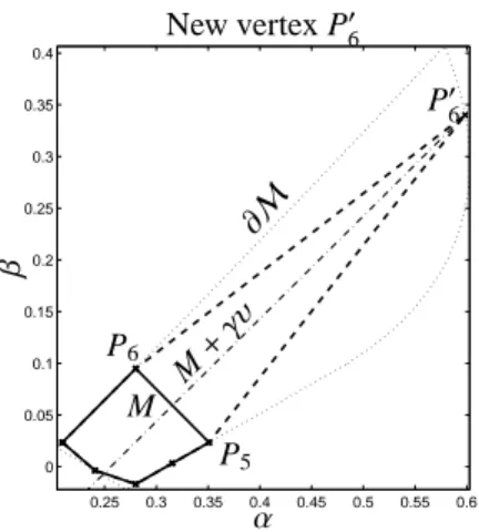
3.4. The polygon inflation: Adding of vertices
The edges of the initial triangle and also the edges of refined polygons are subdivided by introducing new vertices in a way that the refined polygon is a better ap- proximation of the AFS. Next the adding of a new ver- tex is explained. Therefore, let the m-gon P with the vertices (P1, . . . ,Pm) be given. Then P is inflated to an (m+1)-gon P′with the vertices (P′1, . . . ,P′m+1). If the edge between Piand Pi+1is selected for the refinement, then the new vertex P′i+1is a point of intersection of the mid-perpendicular of the edge PiPi+1and the boundary
∂M. The refined polygon has the vertices
(P′1,P′2, . . . ,P′m+1)=(P1,P2, . . . ,Pi,P′i+1,Pi+1, . . . ,Pm).
If P approximates a topologically connected convex subset M, then the new vertex P′i+1 is located not in the interior of P so that the new polygon P′contains P as a subset. In case of a concave boundary element the new polygon P′ may have a smaller area than P. The mid-perpendicular of the edge PiPi+1has the form
M+γυ, γ∈R (10)
with
M=1
2(Pi+Pi+1), υ⊥PiPi+1. 5
0.25 0.3 0.35 0.4 0.45 0.5 0.55 0.6 0
0.05 0.1 0.15 0.2 0.25 0.3 0.35 0.4
α
β
∂M
M M+γυ
P5
P6
P′6 New vertex P′6
Figure 5: Adding of the vertex P′6which is located on the intersection of the mid-perpendicular through P5and P6and the boundary ofM.
The point of intersection of the straight line (10) and
∂Mis not unique (there are two or more points of inter- section); the new vertex P′i+1is determined in a way that the Euclidean distance to M is minimized and that the polygon is not dissected into two parts (to avoid to find a new vertex on the opposite side of the polygon, i.e.
P′i+1M dissects P). Figure 5 illustrates the refinement of a 6-gon to a 7-gon.
The accuracy of a new vertex depends on the func- tion F which is to be minimized along the straight line (10). Numerically we use the relatively slow converg- ing bisection method for the root finding because of its simplicity and robustness. The iteration is stopped if a final accuracyεbis reached so that
P′i+1∈ M, min
x<M
P′i+1−x2< εb. (11)
The number of iterations depends on εb and on the lengthkPi−Pi+1k2 of the edge. In our numerical cal- culations between 3 iterations (for εb = 10−2) and 8 iterations (forεb = 10−5) were needed to determine a vertex P′i+1.
3.5. Adaptive edge selection in the refinement process An adaptive process is used to determine those edges of the polygon whose subdivision promises to improve the approximation of the AFS in the best way. Next a selection strategy is introduced together with a termina- tion criterion.
The central quantity which steers the refinement pro- cess is the change-of-area of the polygon which arises if an edge is subdivided. So if an edge PiPi+1 is sub- divided, then each of the new edges gets a equally
weighted gain-of-area
∆i=1
4kPi−Pi+1k2M−P′i+12 (12) as an attribute. In the next step an edgeℓis selected for which
ℓ=arg max
j ∆j
in order to determine an edge which promises a maxi- mal gain-of-area on the basis of its subdivision history.
If there is no unique indexℓ, then the algorithm starts with the smallest index. As for the initial triangle no subdivision history is available, all three initial edges are subdivided at the beginning.
The refinement process is stopped if the largest achievable gain-of-area drops below some final accu- racyδ. The actual value ofδmay depend on the prob- lem. We often useδ=εb.
3.6. Noisy data
The polygon inflation algorithm works well for non- perturbed as well as for noisy data. The parameter ε in (7) controls the allowance of relative negative con- tributions in C and A and, in our experiments, appears to cause a favorable numerical stability with respect to perturbations.
However, the noise level must be limited in a way that the first three singular vectors V(:,i), i=1,2,3, still contain the essential information on the system. If this is not guaranteed, then the expansion (2) cannot guarantee for a proper reconstruction of C and A. Then even no regular transformation T may exist so that C and A are nonnegative matrix factors.
3.7. Efficiency of the polygon inflation
Three characteristic traits of the polygon inflation al- gorithm are compiled next and are compared with the triangle inclusion method.
1. The polygon inflation algorithm which uses the function (7) has to minimize sums of onlyO(k+n) squares. In contrast to this the function ssq in- cludes O(kn) squares in [10]. (Note that by the definition of the Landau symbol it holds thatO(k+ n)=O(s(k+n)) where s is the number of compo- nents which equals 3 throughout this paper.) 2. Negative entries of C and A larger than−εare not
completely ignored in the polygon inflation algo- rithm but affect the minimum of F, see (8). To show that the ssq function from [10] and the func- tion F (8) result in very similar AFSs, we applied 6
ε M1 M2 M3
0 0 0 0
5·10−3 1.6·10−4 9.3·10−5 1.4·10−4 1·10−2 5.2·10−4 2.8·10−4 4.0·10−4 5·10−2 2.1·10−4 2.2·10−4 1.5·10−4
Table 1: Comparison of the AFS computed with the function F by (8) and the AFS with ssq according to [10]. The Hausdorffdistance of the two AFSs is tabulated for someε. The accuracy of the bound- ary approximation is bounded byεb =10−4. ThereinMiis the ith topologically connected subset ofM.
these algorithms to the model problem from Sec- tion 4 and used the Hausdorffmetric as a measure of distance between these sets. The Hausdorffdis- tance between to sets A and B is
δ(A,B)=max
max
a∈A D(a,B),max
b∈B D(b,A)
where D(x,Y) = miny∈Y(kx−yk2) is the distance of a point x from the set Y. Numerical values of the Hausdorffdistances are listed in Table 1; the distances are very small and the sets coincide ifǫ= 0.
3. The polygon inflation algorithm results in a piece- wise linear interpolation of the boundary ofMby polygons. The local approximation error of a lin- ear interpolation behaves likeO(h2) if the nodes of the interpolant are assumed to be exact. In contrast to this the enclosure of the boundary by a chain of equilateral triangles with the edge-length h results in a final accuracy which is bounded by the width O(h) of this chain.
Further, the local adaptivity of the polygon infla- tion scheme even requires a small number of re- finement steps if the boundary is locally more or less a straight line. A critical nonsmooth region of the boundary can be resolved to any desired accuracy. This adaptive resolution of the bound- ary results in a cost-effective computational proce- dure. In contrast to this number of triangles needed for the triangle inclusion algorithm increases as O(1/h) in the edge length h of the triangles.
3.8. Selection of parameters
Parameters of the polygon inflation algorithm are:
1. The parameterεin (6) controls the degree of ac- ceptable negative entries in the columns of C and the rows of A. Negative matrix elements are not penalized in (7) if their relative magnitude is larger than−ε. This parameter should be increased with
growing perturbations in the spectral data. In our experience 0 ≤ ε ≤ 0.05 seems to be working properly. For model problems and in absence of any errorsε =0 can be used. By construction in- creasingεenlarges the AFS.
2. The parameterεb in (11) controls the quality of the boundary approximation of the AFS. We used εb ≤ 10−3 and sometimesεb ≤ 10−4. The influ- ence of this parameter on the shape and size of the computed AFS is negligible.
3. The parameterδdefines a stopping criterion for the adaptive polygon refinement. If the largest gain-of -area (12) is smaller thanδ, then the refinement can be stopped. We often setδ=εb and state that the shape and size of the computed AFS is not sensi- tive for changes ofδ.
3.9. Two remarks on the numerical implementation 3.9.1. Numerical optimization
Each step of an iterative minimization of F by (8) includes the solution of a nonlinear optimization prob- lem. For a poorly conditioned problem the numerical solutions will scatter around the exact solution. Hence, a new vertex P′i+1might be located in the interior of the AFS in the following sense
minx<M
P′i+1−x2≥εb.
With such an inaccurate vertex the further refinement steps can result in a nonsmooth boundary which may even contain needles directing towards the inside of the AFS. To avoid such misplaced boundary points, we use the powerful optimization procedure NL2SOL [6] and start the iterative minimization with a good initial guess.
A reasonable initial guess can be a convex combination of the numerical solutions which have previously been gained for nearby points. Further, we apply some deci- sion tree before accepting points as valid. Nevertheless, misplaced boundary points can be detected by looking for obtuse angles along the edges of the polygon. Then suspicious vertices may be removed and the optimiza- tion can be restarted.
3.9.2. Weakly separated subregions of the AFS
If parts of the boundary of two isolated subregions of the AFS are in close proximity, then the numerical algorithm tends to agglutinate these regions to a joint connected subset. However, for most of the practical problems the subsets of the AFS appear to be well sep- arated.
7
4. A three-component model problem
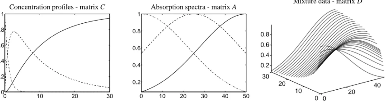
Next the polygon inflation algorithm is applied to a three-component model problem. The total computa- tion time and the number of evaluations of points (α, β) concerning their membership inMis recorded. Further, the accuracy parameters and the noise level are varied.
The results are compared with the triangle enclosing al- gorithm.
4.1. The model problem
We consider the consecutive reactions X −−→K1 Y −−→K2 Z
with the vector of kinetic constants K = (K1,K2) = (1,0.1) and with initial concentrations c(0) = (1,0,0).
Along the time interval [0,30] a number of k = 1000 equidistant nodes is used. The pure component spectra on [0,50] are set to
a1(λ)=exp(− λ2 1000), a2(λ)=exp(−(λ−25)2
1000 ), a3(λ)=exp(−(λ−50)2
1000 ).
The discretization uses n=1500 equidistant nodes. The resulting spectral data matrix D∈ R1000×1500is formed according to
Di j=Ci1A1 j+Ci2A2 j+Ci3A3 j.
Figure 6 shows the factors C and A together with the product matrix D.
4.2. The AFS for C and A
Figure 7 shows the results of a computation of the AFS by means of the polygon inflation algorithm for the concentration factor (MC) and also for the spectral factor (MA). The setsMCandMAare each composed of three isolated and topologically connected subsets.
The associated ranges of possible solutions for the con- centration profiles are shown in Figure 8. A separate concentration profile is drawn for each vertex of the three polygons which approximate the AFS. Addition- ally, a concentration profile is drawn for each node of a quadratic mesh which falls into the AFS. One observes that the area (in the sense of an integral) of connected subsets of the AFS is not directly associated with the size of the area which is enclosed by the series of con- centration profiles. In other words, a large connected
subset of the AFS does not imply strong variations in the associated solutions. This is most evident for the components X and Z (the associated indexes are i = 1 and i = 3). The variability of the concentration pro- files more strongly depends on the variability of the left singular vectors U(:,i), i=1,2,3, of D.
4.3. Variation of the accuracy parameters ε, εb and noisy data
Next a direct comparison is given of the triangle in- clusion algorithm [10] with the polygon inflation algo- rithm from Section 3. Therefore the boundary accuracy parameterεb, see (11), is set toεb = 10−2,10−3,10−4 and the parameter on the acceptance on relative nega- tiveness is set to ε = 5 ·10−12 and 5·10−3, see (6).
In our implementation of the triangle inclusion algo- rithm the parameter εb is the side-length of the equi- lateral triangles. BothMC andMA are computed and the required number of program calls of F (funcalls) is recorded, see Table 2. Further, the computation time on a standard PC with a 2.4GHz Intel CPU with 16 GB RAM is tabulated. The program code has been writ- ten in C and some FORTRAN libraries are used. For the triangle inclusion algorithm the number of funcalls is equal to the number of vertices of the triangles en- closing the boundary of the AFS. In the polygon infla- tion algorithm multiple funcalls are needed to find a new vertex on the boundary of the AFS by means of the bi- section algorithm. However, its total number is always smaller than that for the triangle inclusion approach. If the accuracy parameter εb is decreased by one power of 10, then in our implementation of the triangle inclu- sion scheme the number of funcalls increases with the factor of about 10; in contrast to this the number of fun- calls increases with the factor of less than √
10 for the polygon inflation scheme. All these results appear to be stable if the data are slightly perturbed or if the con- trol parameters for relative negativeness are increased.
Figure 9 shows the AFS for the spectral factor A if the control parameters for relative negativeness are set to ε∈ {0.05,0.04,0.03,0.02,0.01,0}.
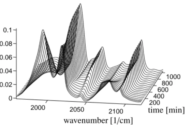
5. Rhodium-catalyzed hydroformylation
The kinetics of the hydroformylation of 3,3- dimethly-1-butene with a rhodium/tri(2,4-di-tert- butylphenyl)phosphite catalyst in n-hexane has been studied in detail in [18]. The in situ FTIR spectroscopic data from this publication are reused for a computation of the AFS; for additional information on the reaction conditions and on the experimental HP FTIR apparatus see [18].
8
0 10 20 30 0
0.2 0.4 0.6 0.8 1
Concentration profiles - matrix C
0 10 20 30 40 50
0.2 0.4 0.6 0.8 1
Absorption spectra - matrix A
0 20
40 0
10 20 30 0.2 0.4 0.6 0.8
Mixture data - matrix D
Figure 6: The matrix factors C and A with dash-dotted line for the component X, dashed line for Y and solid line for Z. The right figure shows the product/absorption data D.
−3 −2 −1 0
0 0.5 1 1.5 2 2.5 3
α
β
AFSMCfor the concentration factor C
(X)
(Y)
(Z)
−1.5 −1 −0.5 0 0.5
−0.4
−0.2 0 0.2 0.4 0.6 0.8 1
α
β
AFSMAfor the spectral factor A
(X)
(Y)
(Z)
Figure 7: Left: The area of feasible solutionsMCfor the concentration factor C. Right: The area of feasible solutionsMAfor the spectral factor A.
For the concentration profiles the solution with the smallest integrated absolute value of the curvature and for which only one reactant is nonzero at time zero have been marked by a small circle. The three associated points in the AFSMAare also marked with a circle.
0 10 20 30
0 0.2 0.4 0.6 0.8 1
t
Feasible concentration profiles X
0 10 20 30
0 0.02 0.04 0.06 0.08
t
Feasible concentration profiles Y
0 10 20 30
0 0.01 0.02 0.03 0.04
t
Feasible concentration profiles Z
Figure 8: Feasible concentration profiles C(:,i) for the three components i=1 for X, i=2 for Y and i=3 for Z according to the three topologically connected subsets of the AFSMCin the left side of Figure 7. The area of a connected subset of the AFS is not correlated with the variability of the range of feasible solutions for the associated component, cf. Section 4.2.
withε=10−12 withε=5·10−3
Triangle inclusion Polygon inflation Triangle inclusion Polygon inflation εb funcalls time [s] funcalls time [s] vertices funcalls time [s] funcalls time [s] vertices Factor
A
10−2 1166 13 352 4 65 1218 13 409 4 81
10−3 11566 83 1314 12 197 12168 89 1346 11 205
10−4 115658 660 3413 26 411 121685 685 4001 32 479
factor C
10−2 2334 19 1541 12 81 2733 22 626 7 117
10−3 23258 153 1966 18 229 27229 178 1666 16 233
10−4 232477 1341 4465 44 467 272897 1609 4541 44 507
Table 2: The number of program calls ofF(funcalls) in order to compute (9) is tabulated for varyingεb together with the required computing time. The termination is controlled byδ=εb, see Section 3.5. The ratios of required computing time and funcalls is not constant as for computations with higher accuracy better initial values are available. Then convergence can be achieved with only a small number of iterations.
9
−2 −1.5 −1 −0.5 0 0.5 0
0.5 1 1.5
α
β
Figure 9: Some different areas of feasible solutions for the factor A for perturbed data and withε∈ {0.05,0.04,0.03,0.02,0.01,0}.
5.1. The FTIR data
We use a spectroscopic data set which contains char- acteristic absorptions from three components, namely the olefin, the acyl complex and the hydrido complex.
A total number of k = 1045 spectra is used and each spectrum contains n=664 spectral channels within the wavenumber interval [1960,2120]cm−1. The sequence of spectra is shown in Figure 10. The spectroscopic data matrix D∈R1045×664is the basis for the computation of the AFS for a three-component system.
5.2. Computation of the AFS and ranges of feasible so- lutions
As explained in Section 3.3 a first nonnegative factor- ization D=CA is to be computed for the initialization.
This can be done by standard factorization tools like the PCD code [24] or by the MCR-ANLS algorithm [15], the SPECFIT code [3] or even by the NNMF code [17]
written in Matlab. For the given spectroscopic data the permissibility of small negative entries in the factors C and A appears to be important; we useε=0.01 in (6).
Further, the boundary approximation parameter (11) is set toεb =10−4. The termination parameter isδ=10−4, see Section 3.5.
Figure 11 shows the two areas of feasible solutions MCandMA. No a priori information has been used for the decomposition, e.g., no mass balance for rhodium is taken into account. The total computation times (the same hardware as in Section 4 is used) are 24.3 seconds forMC and 25.0 seconds forMA. The polygonMCis spanned by 479 vertices and 3897 funcalls are needed
2000 2050 2100
200 400
600 800
1000
0 0.02 0.04 0.06 0.08 0.1
wavenumber [1/cm]
time [min]
Sequence of absorption spectra
Figure 10: Hydroformylation of 3,3-dimethly-1-butene. Series of FTIR spectra which is determined by three components (olefin, acyl complex and hydrido complex). See Figure 2 in [18] for an assign- ment of the peaks to the components as well as for the experimental and spectroscopic details.
for its computation; the polygonMA contains 417 ver- tices with 3487 funcalls.
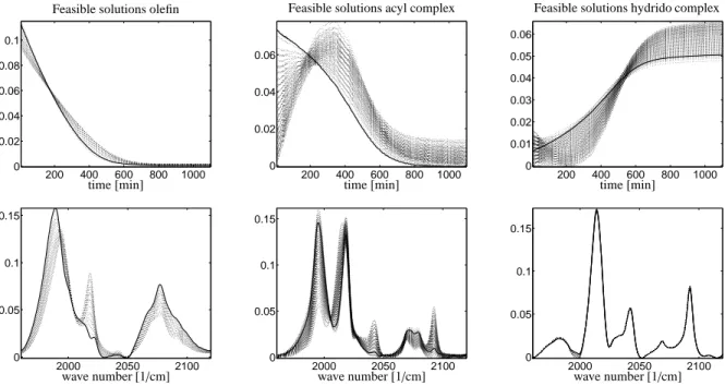
In MA only a very small subset, marked by (c), is responsible for the absorption spectrum of the hydrido complex. The corresponding spectrum appears to be nearly unique, see right lower spectrum in Figure 12;
an explanation can be derived from the relative concen- trations at the end of the reaction and from the isolation of certain peaks in the spectrum of the hydrido complex compared to the spectra of the other components.
This corresponds with a very small range of possi- ble concentration profiles for the olefin, see left upper plot in Figure 12. All other ranges for the concentration profiles and spectra are also shown in Figure 12. As in Section 4.2 a separate concentration profile or spec- trum is drawn for each vertex of the AFS. Additionally, a concentration profile or spectrum is plotted for each node of a quadratic mesh which is located in the AFS.
Within each plot the smoothest solution with the small- est integral of the absolute value of the discrete second derivative has been plotted by a bold line.
6. Conclusion
A new fast numerical scheme for the adaptive approx- imation of the AFS for three-component systems by a sequence of polygons has been introduced. Piecewise linear interpolation of the boundary of the AFS results in a local approximation error which behaves likeO(h2) if h is the distance of adjacent vertices. Further, local adaptivity allows to reduce the number of vertices which 10
−1 −0.5 0 0.5 1
−0.8
−0.6
−0.4
−0.2 0 0.2 0.4
α
β
AFSMCfor the concentration factor C (a)
(b)
(c)
−0.8 −0.6 −0.4 −0.2 0 0.2 0.4
−0.4
−0.2 0 0.2 0.4 0.6
α
β
AFSMAfor the spectral factor A
(a)
(b)
(c)
Figure 11: Hydroformylation of 3,3-dimethly-1-butene with an analysis of a three-component subsystem consisting of the olefin, the acyl complex and the hydrido complex. Left: The area of feasible solutionsMCfor the concentration factor. Right: The area of feasible solutionsMAfor the spectral factor.
InMCthe concentration profiles with the smallest integrated absolute value of the curvature have been marked by a circle. The three associated points in the AFSMAare also marked by a circle. Each of three separated subsets ofMCandMAare associated with a specific component. The subset (a) represents the olefin, (b) represents the acyl complex and (c) marks the hydrido complex.
200 400 600 800 1000 0
0.02 0.04 0.06 0.08 0.1
time [min]
Feasible solutions olefin
200 400 600 800 1000 0
0.02 0.04 0.06
time [min]
Feasible solutions acyl complex
200 400 600 800 1000 0
0.01 0.02 0.03 0.04 0.05 0.06
time [min]
Feasible solutions hydrido complex
2000 2050 2100
0 0.05 0.1 0.15
wave number [1/cm] 2000 2050 2100
0 0.05 0.1 0.15
wave number [1/cm] 2000 2050 2100
0 0.05 0.1 0.15
wave number [1/cm]
Figure 12: Ranges of the feasible concentration profiles (three upper figures) and ranges of feasible spectra (three lower figures). Left figures:
the olefin 3,3-dimethly-1-butene. Middle figures: the acyl complex. Right figures: the hydrido complex. All the ordinates of figures are scaled relatively so that no absolute values on the concentration of absorption should be extracted. No additional information on the reaction system has been used for the decomposition; especially no mass balance on rhodium is taken into account.
11
are needed to approximate the boundary whenever the boundary is smooth. Numerical calculations show con- siderable saving in the computation time for the new polygon inflation scheme. For instance for the problem from Section 5 with a 1045×664 data matrixMCand MAcan be computed in only 50 seconds.
The polygon inflation technique can be generalized to a polyhedron inflation scheme in order to approximate the AFS in case of an s-component system with s≥4.
Local adaptive refinement of the faces of the polyhedron can be applied in a way comparable to three-component systems. Finally, we would like to comment that the non-uniqueness of the solutions in an AFS can be re- duced if any supplemental information on the system is available; see [28] for some complementarity and cou- pling theorems.
References
[1] H. Abdollahi, M. Maeder, and R. Tauler. Calculation and Mean- ing of Feasible Band Boundaries in Multivariate Curve Res- olution of a Two-Component System. Analytical Chemistry, 81(6):2115–2122, 2009.
[2] M.W. Berry, M. Browne, A.N. Langville, V.P. Pauca, and R.J.
Plemmons. Algorithms and applications for approximate non- negative matrix factorization. Computational Statistics and Data Analysis, 52:155–173, 2007.
[3] R.A. Binstead, B. Jung, and A.D. Zuberb¨uhler. SPECFIT/32 Global analysis system. Spectrum Software Associates, Chapel Hill, NC, USA, 2000.
[4] O.S. Borgen, N. Davidsen, Z. Mingyang, and Ø. Øyen.
The multivariate N-Component resolution problem with min- imum assumptions. Microchimica Acta, 89:63–73, 1986.
10.1007/BF01207309.
[5] O.S. Borgen and B.R. Kowalski. An extension of the multivari- ate component-resolution method to three components. Analyt- ica Chimica Acta, 174(0):1–26, 1985.
[6] J. Dennis, D. Gay, and R. Welsch. Algorithm 573: An adaptive nonlinear least-squares algorithm. ACM Transactions on Math- ematical Software, 7:369–383, 1981.
[7] H. Gampp, M. Maeder, C.J. Meyer, and D. Zuberb¨uhler. Cal- culation equilibrium constants from multi-wavelength spec- troscopy data I, Mathematical considerations. Talanta, 32:95–
101, 1985.
[8] P.J. Gemperline. Computation of the Range of Feasible Solu- tions in Self-Modeling Curve Resolution Algorithms. Analytical Chemistry, 71(23):5398–5404, 1999.
[9] P.J. Gemperline and E. Cash. Advantages of soft versus hard constraints in self-modeling curve resolution problems. Alter- nating least squares with penalty functions. Anal. Chem., 75:4236–4243, 2003.
[10] A. Golshan, H. Abdollahi, and M. Maeder. Resolution of Ro- tational Ambiguity for Three-Component Systems. Analytical Chemistry, 83(3):836–841, 2011.
[11] A. Golshan, H. Abdollahi, and M. Maeder. The reduction of ro- tational ambiguity in soft-modeling by introducing hard models.
Analytica Chimica Acta, 709(0):32–40, 2012.
[12] G.H. Golub and C.F. Van Loan. Matrix computations. Johns Hopkins University Press, Baltimore, MD, third edition, 1996.
[13] H. Haario and V.M. Taavitsainen. Combining soft and hard modelling in chemical kinetics. Chemometr. Intell. Lab., 44:77–
98, 1998.
[14] J.C. Hamilton and P.J. Gemperline. Mixture analysis using fac- tor analysis. II: Self-modeling curve resolution. J. Chemomet- rics, 4(1):1–13, 1990.
[15] J. Jaumot and R. Tauler. MCR-BANDS: A user friendly MAT- LAB program for the evaluation of rotation ambiguities in Mul- tivariate Curve Resolution. Chemometrics and Intelligent Lab- oratory Systems, 103(2):96–107, 2010.
[16] A. Juan, M. Maeder, M. Mart´ınez, and R. Tauler. Combining hard and soft-modelling to solve kinetic problems. Chemometr.
Intell. Lab., 54:123–141, 2000.
[17] H. Kim and H. Park. Nonnegative matrix factorization based on alternating nonnegativity constrained least squares and active set method. SIAM J. Matrix. Anal. Appl., 30:713–730, 2008.
[18] C. Kubis, D. Selent, M. Sawall, R. Ludwig, K. Neymeyr, W. Baumann, R. Franke, and A. B¨orner. Exploring between the extremes: Conversion dependent kinetics of phosphite-modified hydroformylation catalysis. Chemistry - A Europeen Journal, 18(28):8780–8794, 2012.
[19] W.H. Lawton and E.A. Sylvestre. Self modelling curve resolu- tion. Technometrics, 13:617–633, 1971.
[20] M. Maeder and Y.M. Neuhold. Practical data analysis in chem- istry. Elsevier, Amsterdam, 2007.
[21] E. Malinowski. Factor analysis in chemistry. Wiley, New York, 2002.
[22] R. Manne. On the resolution problem in hyphenated chro- matography. Chemometrics and Intelligent Laboratory Systems, 27(1):89–94, 1995.
[23] H. Minc. Nonnegative matrices. John Wiley & Sons, New York, 1988.
[24] K. Neymeyr, M. Sawall, and D. Hess. Pure component spectral recovery and constrained matrix factorizations: Concepts and applications. J. Chemometrics, 24:67–74, 2010.
[25] R. Rajk´o. Studies on the adaptability of different Borgen norms applied in self-modeling curve resolution (SMCR) method. J.
Chemometrics, 23(6):265–274, 2009.
[26] R. Rajk´o and K. Istv´an. Analytical solution for determining fea- sible regions of self-modeling curve resolution (SMCR) method based on computational geometry. J. Chemometrics, 19(8):448–
463, 2005.
[27] M. Sawall, A. B¨orner, C. Kubis, D. Selent, R. Ludwig, and K. Neymeyr. Model-free multivariate curve resolution com- bined with model-based kinetics: algorithm and applications.
J. Chemometrics, 26:538–548, 2012.
[28] M. Sawall, C. Fischer, D. Heller, and K. Neymeyr. Reduction of the rotational ambiguity of curve resolution technqiues under partial knowledge of the factors. Complementarity and coupling theorems. J. Chemometrics, 26:526–537, 2012.
[29] R. Tauler. Calculation of maximum and minimum band bound- aries of feasible solutions for species profiles obtained by mul- tivariate curve resolution. J. Chemometrics, 15(8):627–646, 2001.
[30] M. Vosough, C. Mason, R. Tauler, M. Jalali-Heravi, and M. Maeder. On rotational ambiguity in model-free analyses of multivariate data. J. Chemometrics, 20(6-7):302–310, 2006.
12

![Table 1: Comparison of the AFS computed with the function F by (8) and the AFS with ssq according to [10]](https://thumb-eu.123doks.com/thumbv2/1library_info/4870983.1632598/7.918.120.408.89.181/table-comparison-afs-computed-function-afs-ssq-according.webp)