Does the signal contribution function attain its extrema on the boundary of the area of feasible solutions?

Does the signal contribution function attain its extrema on the boundary of the area of feasible solutions?

Klaus Neymeyr^a,b, Azadeh Golshan^c, Konrad Engel^a, Rom`a Tauler^d, Mathias Sawall^a

aUniversit¨at Rostock, Institut f¨ur Mathematik, Ulmenstrasse 69, 18057 Rostock, Germany

bLeibniz-Institut f¨ur Katalyse, Albert-Einstein-Strasse 29a, 18059 Rostock

cUniversity of Newcastle, Department of Chemistry, Callaghan, NSW 2308, Australia

dInstitute of Environmental Assessment and Water Research, Spanish Council of Research, Jordi Girona 18, 08034 Barcelona, Spain

Abstract

The signal contribution function (SCF) was introduced by Gemperline in 1999 and Tauler in 2001 in order to study band boundaries of multivariate curve resolution (MCR) methods. In 2010 Rajk´o pointed out that the extremal profiles of the SCF reproduce the limiting profiles of the Lawton-Sylvestre plots for the case of noise-free two-component systems.

This paper mathematically investigates two-component systems and includes a self-contained proof of the SCF- boundary property for two-component systems. It also answers the question if a comparable behavior of the SCF still holds for chemical systems with three components or even more components with respect to their area of feasible solutions. A negative answer is given by presenting a noise-free three-component system for which one of the profiles maximizing the SCF is represented by a point in the interior of the associated area of feasible solutions.

Key words: signal contribution function, multivariate curve resolution, Lawton-Sylvestre plot, Borgen plot, Area of feasible solutions, MCR-Bands, FACPACK

1. Introduction

The following question on the solution ambiguity underlying multivariate curve resolution (MCR) methods ap- pears to be still open:

“Is it true that the maximum and the minimum of the signal contribution function (SCF) as computed by MCR-Bands are always attained in profiles represented by boundary points of the associated area of feasible solutions?”

The question emerged after the proposal of Gemperline in 1999 [1] for the calculation of the range of feasible solutions in self-modelling curve resolution by using the integrated signal of every constituent and was further devel- oped by Tauler in 2001 [2] with the maximization and minimization of the scaled signal contribution function (SCF).

The meaning of the maximum and minimum SCF boundaries was afterwards examined in detail for two-component systems [3, 4] for which the area of feasible solutions can be represented in the form of a Lawton-Sylvestre plot.

Simultaneously Rajk´o [5] pointed out that for systems with two components, the profiles that minimize and maximize the SCF are represented by the cone boundaries of the Lawton-Sylvestre (LS) plots [6]. This strong relationship of LS-plots and the maximal/minimal profiles resulting from MCR-Bands, which in some sense “enclose” the solution ambiguity of an MCR method, is the basis for the question whether a comparable property still holds for systems with three or more chemical components. For three-component systems the LS-plots find their natural generalization in Borgen plots or more generally the Area of Feasible Solutions (AFS) [7, 8, 9, 10, 11, 12]. Then the question is whether the extremal profiles of MCR-Bands are represented by points on the boundary of the associated AFS. This problem has also been discussed between participants of the CAC 2016 (Barcelona) and TIC 2017 (Newcastle) conferences and the authors.

This paper shows that the extremal profiles of the SCF for two-component systems are represented by the boundary lines of the associated Lawton-Sylvestre plots and that the extremal profiles for systems with three and more compo- nents are not always represented by points on the boundary of the AFS. In some sense, the present analysis combines the two approaches for representing the solution ambiguity of MCR methods, namely the band representation for the feasible solutions and the singular value decomposition based representation. The latter approach represents the ranges of feasible solutions by the expansion coefficients with respect to the spaces of left and right singular vectors.

July 18, 2019

1.1. Overview

First, Section 2 introduces the theoretical background. Section 3 contains a proof (on the basis of the Perron- Frobenius spectral theory of nonnegative matrices) that the SCF takes its extrema in the profiles represented by the boundary lines of the Lawton-Sylvestre cones. Finally, Section 4 gives a negative answer to the above question by presenting a model problem that does not fulfill the desired property.

2. Theoretical background

The spectral mixture data of an s-component chemical system is assumed to be stored in a nonnegativek×n matrixD. The MCR problem is to determine the pure component factors of the concentration profilesC ∈R^k×sand the associated spectraS ∈R^n×saccording to the Lambert-Beer law that reads for the noise-free case

D=CS^T. (1)

For the following analysis a crucial assumption on the matrixDhas to be made, namely thatD^TDis an irreducible matrix [13]. Irreducibility means thatD^TDcannot be transformed to a block-diagonal matrix by simultaneous and equal permutations of the columns and rows, see Appendix A for details. From a chemical point of view, this ex- presses that the spectral mixture data cannot be separated by reordering the measurements and the channel indices into completely independent subsystems.

A possible first step in solving the factorization problem (1) is to compute a singular value decomposition (SVD) D=UΣV^TofDwith thek×kmatrixUof the left singular vectors, thek×ndiagonal matrixΣof the singular values and then×nmatrixVof the right singular vectors. Any factorization (1) ofDcan be represented on the basis of the SVD by means of a regular 2-by-2 block matrixT ∈R^s×sso thatC=UΣT⁻¹andS^T =T V^T. Therein,Thas the form

T = 1 x

1 W

!

(2) with the row vectorx=(x1, . . . ,xs−1) and the all-ones column vector1 =(1, . . . ,1)^T ∈R^s−1, see [7, 4, 9, 14]. The first column ofT needs a justification asS^T =T V^T implies that any spectral profile has a contribution from the first right singular vector. This has been shown in Thm. 2.2 of [14] by using, again, the irreducibility of D^TDand the Perron-Frobenius theorem on nonnegative matrices, cf. Appendix A.

A low-dimensional representation of all feasible spectral profiles is the Borgen plot [7, 4] in the case of a three- component system. In the general case ofs-component systems this low-dimensional representation is a subset of the (s−1)-dimensional space and is called the Area of Feasible Solution (AFS)

MS =n

x∈R^s−1: W ∈R(s−1)×(s−1)

exists in (2) such thatT is regular andC,S ≥0o .

Nonnegativity is the decisive constraint onCandS. Similarly, the corresponding representation of the set of feasible concentration profiles reads

MC=n

y∈R^s−1: a regular matrixT ∈R^s×sexists with (T⁻¹)(:,1)=(1,y^T)^T andC,S ≥0o .

The setsM_S andM_C can be constructed geometrically (Borgen plots) [7, 8, 15, 16] or can be approximated nu- merically by the grid-search method [17, 3], the triangle enclosure method [9, 18], the polygon inflation algorithms [10, 14] or by the ray-casting approach [19]. See [11, 12, 20] for further details.

2.1. The signal contribution function

Gemperline [1] and Tauler [2] have suggested approaches for determining feasible profiles with a minimal and maximal integrated signal or relative signal contribution. The signal contribution function (SCF) has the form kcis^T_ikF/kCS^TkF whereci and si are the concentration profile and the spectrum of theith component. In the case of noise-free data with rank(D) = s, the concentration profileci can be written as a linear combination of the left singular vectors (in scaled form this is a linear combination of the columns ofUΣ) and the associated spectrumsi, which is a linear combination of the right singular vectors. Then the SCF can be written as

g_i(T)=

UΣ(T⁻¹(:,i))(T(i,:))V^T2_F

CS^T2_F (3)

fori ∈ {1, . . . ,s}and with T ∈ R^s×s. Thereink · k²_F is the squared Frobenius norm, i.e., the sum of squares of all matrix elements. For a chemical system with s components, the functionsg_i are minimized and maximized

2

fori = 1, . . . ,sunder the nonnegativity constraints thatUΣT⁻¹ ≥ 0 andT V^T ≥ 0. This results in 2sextremal concentration profiles (eachsfor the minima and sfor the maxima) and analogously 2sextremal spectral profiles.

The constrained minimization/maximization is implemented in the MCR-Bands software [21] and works with the MatLaboptimization routinefmincon.

The resulting extremal profiles can be represented in a low-dimensional way in the AFS. Letci∈R^k,i=1, . . . ,2s, be the extremal concentration profiles and si ∈ Rⁿ, i = 1, . . . ,2s, be the associated spectral profiles. Their low- dimensional representatives [15, 16] in the AFS are

x⁽ⁱ⁾= (V(:,2 : s))^Tsi

(V(:,1))^Ts_i , y⁽ⁱ⁾ =U(Σ(:,2 : s))ci

U(Σ(:,1))ci

, i=1, . . . ,2s. (4)

One typically observes that the profile representing vectorsx⁽ⁱ⁾ andy⁽ⁱ⁾ are located on the boundary of the AFS. For two-component systems this is examined numerically in [3] and systematically analyzed in [5].

3. The SCF for two-component systems 3.1. The SCF

ForC=UΣT⁻¹andS^T =T V^Tand

T = 1 α

1 β

!

, T⁻¹= 1

β−α

β −α

−1 1

!

(5) withα,β, which guarantees regularity ofT, we getC∈R^k×2andS ∈R^n×2

C=(c1,c2)=UΣT⁻¹= 1

β−α(βσ1u1−σ2u2,−ασ1u1+σ2u2), S^T = s^T₁

s^T₂

!

=T V^T = 1 α

1 β

! 3^T

1

3^T

2

!

= 3^T

1 +α3^T

2

3^T

1 +β3^T

2

! .

(6)

The numerator of the signal contribution function (3) can be simplified as for any column-vectorsa∈R^kandb∈Rⁿ it is true thatkab^Tk_F =kak₂kbk₂. Thus we get

kc₁s^T₁k²_F =kc₁k²₂ks₁k²₂=(β²σ²₁+σ²₂)(1+α²)

(β−α)² =:eg₁(α, β), kc2s^T₂k²_F =kc2k²₂ks2k²₂=(α²σ²₁+σ²₂)(1+β²)

(β−α)² =:eg2(α, β).

(7)

In order to study the SCF (3), we can omit theT-independent (and therefore constant) denominatorkCS^Tk²_F =kDk²_F since extrema ofgi(T) are attained in the same (α, β) as extrema ofegi(α, β) by (7). Further the symmetry property

eg1(α, β)=eg2(β, α) provides the justification to restrict the analysis only on finding extrema of

h(α, β) :=UΣ(T⁻¹(:,1))(T(1,:))V^T2_F =kc1s^T₁k²_F =kc1k²₂ks1k²₂ (8) since any extremal point ofh(α, β) is an extremal point ofeg2(β, α) and vice versa, see also [3].

3.2. Extrema of the SCF are attained on the boundary of the feasible-solutions-rectangle

The nonnegativity constraintsC≥0 andS ≥0 imply strong restrictions on (α, β). These restriction have the form (α, β)∈[a,b]×[c,d] or (β, α)∈[a,b]×[c,d],

see, e.g., Sec. 3.6 in [14], with a=−min

Vi2>0 i=1,...,n

Vi1

Vi2

, b= min

i=1,...,k

Ui2σ2

Ui1σ₁ <0, c= max

i=1,...,k

Ui2σ2

Ui1σ₁ >0, d=−max

Vi2<0 i=1,...,n

Vi1

Vi2

. (9)

3

Our aim is to show that extrema ofh(α, β) by (8) cannot be attained in the interior of the rectangle [a,b]×[c,d] but on its boundary. To prove this, we assume that an extremum is attained in an interior point and derive a contradiction.

A necessary condition for an extremum in an interior point is a vanishing gradient vector, namely

∇h=





∂h

∂α

∂h

∂β



= 2 (α−β)³

−(β²σ²₁+σ²₂)(αβ+1) (αβσ²₁+σ²₂)(1+α²)

!

=0. (10)

The factor (β²σ²₁+σ²₂)≥σ²₂in the first component is strictly positive so that

αβ=−1. (11)

In the second component, (1+α²)>0 implies that the first factor must be zero. Hence with (11) we get thatσ²₁ =σ²₂. This contradicts the Perron-Frobenius theorem, see Appendix A, as the largest eigenvalueσ1of the irreducible matrix D^TDis a simple (non-degenerate) eigenvalue. Thus no local extremum can be attained in the interior of [a,b]×[c,d].

3.3. The maximum and minimum of the SCF are attained in the vertices of the feasible-solutions-rectangle

So far, we know that extrema (ξ, η) of the SCF are attained on the boundary of the rectangle [a,b]×[c,d] so that (ξ, η) have the forms

(a, η) or (b, η) withc≤η≤d, (left and right vertical edges), or alternatively (ξ,c) or (ξ,d) witha≤ξ≤b, (upper and lower horizontal edges).

However, if an extremum were attained in an edge-point that is not a vertex, then the SCF extremal profile would not include the associated band of feasible solutions.

Next we show that the minimum and the maximum of the SCF are attained in two vertices of the rectangle [a,b]×[c,d]. To this end, the partial derivatives∂h/∂αand∂h/∂βare proved to be strictly monotone functions on the edges of the rectangle [a,b]×[c,d]. By (10) we get that

∂h

∂α= 2

(β−α)³(β²σ²₁+σ²₂)(1+αβ), ∂h

∂β =− 2

(β−α)³(αβσ²₁+σ²₂)(1+α²).

If these derivatives do not have a zero on the boundary of [a,b]×[c,d], then each of the restrictions of h to the edges of the rectangle is a monotone function. A zero in a vertex is possible as this does not interfere with the strict monotonicity. Since

β−α >0 by α≤b<0<c≤β, β²σ²₁+σ²₂> σ²₂>0 and 1+α²>1>0 it remains to show that

1+αβ,0 and αβσ²₁+σ²₂ ,0 (12)

on the boundary of the rectangle (apart form the endpoints). These two inequalities are proved in the following. For the mathematical analysis, we need the next properties of the columns ofUandV.

Property 3.1. Let3₁and3₂be the column vectors of V. Applying the Perron-Frobenius theorem, see Theorem A.2, to the matrix A=D^TD the vector3₁ is a component-wise positive vector (use−3₁if the SVD yields a component-wise negative vector). Then the orthogonality property3^T

13₂ =0implies that the vector3₂has positive and also negative components (as otherwise the sum of the inner product would be nonzero). The same properties hold for the columns u1and u2of U by Theorem A.2 if applied to A=DD^T.

Proof thatαβ >−1 on the rectangle [a,b]×[c,d] (apart from the vertices): Fig. 1 shows the limit curveαβ = −1, namelyβ=−1/α, in the (α, β)-plane as the lower boundary of the blue area. If we can show that

ad≥ −1, (13)

where (a,d) are the coordinates of the left upper vertex of the rectangle, then the rectangle [a,b]×[c,d] is located below the limit curveαβ=−1 and at the most its vertex (a,d) can lie on this curve. After insertion of (9) in (13) we have to prove that

minVi2>0 i=1,...,n

Vi1

Vi2

·max

Vi2<0 i=1,...,n

Vi1

Vi2

≥ −1.

4

a b

c d

α β

A

^{< 0}

^{> 0}

∂h

∂β

> 0

∂h

∂β

< 0

B C

Figure 1: The rectangle [a,b]×[c,d] of nonnegative profiles together with the limit curvesβ=−1/α(lower boundary of the blue areaA) together with the limit curveβ=−(σ2/σ1)²/α(upper boundary of the red areaC). The white areaBincludes the rectangle [a,b]×[c,d]. There∂h/∂α >0 and∂h/∂β <0 are true.

For the following transformation of this inequality we use Property 3.1, namely thatVi1>0 for alliand that the second column ofVhas positive and also negative entries. Therefore the first factor on the left side of the last inequality is positive and the second factor is negative. Thus we get

1≤ 1

minVi2>0

i=1,...,n

Vi1

Vi2

· −1

maxVi2<0

i=1,...,n

Vi1

Vi2

.

A reformulation of the two quotients yields

1≤max

Vi2>0 i=1,...,n

Vi2

V_i1 ·(−1)·min

Vi2<0 i=1,...,n

Vi2

V_i1 and further

maxVi2>0 i=1,...,n

Vi2

Vi1

·max

Vi2<0 i=1,...,n

−Vi2

Vi1

≥1.

In this form the assumptions on theVi2can be skipped without changing the maxima. Hence it remains to prove

i=1,...,nmax Vi2

Vi1

· max

i=1,...,n

−Vi2

Vi1

≥1. (14)

See Appendix B for the proof of this inequality.

We conclude that

∂h

∂α= 2

(β−α)³(β²σ²₁+σ²₂)(1+αβ)>0

holds below the limit curveαβ=−1 where the rectangle [a,b]×[c,d] is located. This area is marked byBin Figure 1. In addition, we get that∂h/∂α <0 in the area marked byAin Figure 1.

Next we prove the second inequality in (12) in a similar way.

Proof thatαβσ²₁+σ²₂,0 on the rectangle [a,b]×[c,d] (apart from the vertices): Fig. 1 illustrates the limit curve β=− σ2

σ1

!2

1

α (15)

as the upper boundary curve of the red area. In order to prove the desired property it suffices to prove that c≥ − σ2

σ₁

!2

1 b

where (b,c) are the coordinates of the right lower vertex of the rectangle. The limit case of equality can be accepted since a zero of the partial derivative in the vertex (b,c) does not contradict the assertion. With (9) we have to prove that (withb<0)

i=1,...,kmin U_i2σ₂ Ui1σ1

i=1,...,kmax U_i2σ₂ Ui1σ1

≤ − σ₂ σ1

!2

5

α β

h(α, β) (a,d)

(b,c)

∂h

∂α >0

∂h

∂β <0

Figure 2: The minimum of the SCF on the rectangle [a,b]×[c,d] is taken in the point (a,b) and the maximum is taken in the point (b,c).

or equivalently (with Property 3.1)

i=1,...,kmin Ui2

Ui1

| {z }

<0

· max

i=1,...,k

Ui2

Ui1

| {z }

>0

≤ −1.

By multiplication with−1 together withUi1 >0 for alliand minUi2 <0 by Property 3.1 this yields the following inequality

i=1,...,kmax−Ui2

Ui1

· max

i=1,...,k

Ui2

Ui1

≥1. (16)

This inequality is of the same form as inequality (14); see Appendix B.

We conclude that

∂h

∂β =− 2

(β−α)³(αβσ²₁+σ²₂)(1+α²)<0

above the limit curve (15) where the rectangle [a,b]×[c,d] is located. This area is marked byBin Figure 1. Further, we get that∂h/∂β >0 in the areaCin Figure 1.

3.4. Bounding profiles

On the basis of the strict monotonicity of the SCF on the four edges of the rectangle [a,b]×[c,d] as proved in Section 3.3 we conclude that the SCF attains its minimum in (a,d) and its maximum in (b,c). These relations are illustrated in Figure 2.

For the representation of the bounding profiles we still have to implement a scaling for the concentration factor so that the first row of the modified matrix of expansion coefficients equals the all-ones vector. By multiplyingT⁻¹in (5) with the matrix

∆ =(β−α) 1/β 0

0 −1/α

!

we get

e

T⁻¹:=T⁻¹∆ = β −α

−1 1

! 1/β 0

0 −1/α

!

= 1 1

−1/β −1/α

! .

Then the feasible profiles are represented asC=UΣeT⁻¹andS =VT^T according to (6). For (α, β)=(a,d) we get the SCF-minimizing boundsCandS as

C=(c₁,c₂)=(σ1u1−σ2u2/d, σ1u1−σ2u2/a), S =(s₁,s₂)=(3₁+a3₂,3₁+d3₂).

Similarly, the SCF-maximizing boundsCandS are for (α, β)=(b,c)

C=(c1,c₂)=(σ1u₁−σ₂u₂/c, σ₁u₁−σ₂u₂/b), S =(s1,s2)=(3₁+b3₂,3₁+c3₂).

6

The associated series of bands are as follows: The bands of spectra are represented as s1(α)=3₁+α3₂, α∈[a,b],

s2(β)=3₁+β3₂, β∈[c,d] (17)

and the bands of concentration profiles by

c1(β)=σ₁u1−σ₂u2/β, β∈[c,d],

c2(α)=σ1u1−σ2u2/α, α∈[a,b]. (18) An SCF-minimizing profile is not automatically a lower bound for the band of profiles (the same holds for the SCF- maximizing profiles) since in an isosbestic point the relations may change. Therefore the band inclusions read as follows:

min(s₁,s1)≤s₁(α)≤max(s₁,s1), min(s₂,s2)≤s2(β)≤max(s₂,s2), min(c₁,c₁)≤c₁(β)≤max(c₁,c₁), min(c₂,c2)≤c₂(α)≤max(c₂,c2).

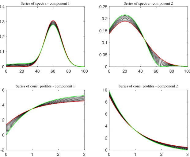
For an illustration see Figure 3. There we consider a two-component model problem with the concentration profile c1(t)=exp(−t) andc2=1−c1(t). The two spectra ares1(λ)=exp(((λ−60)/15)²) ands2(λ)=exp(((λ−20)/35)²).

The mixture data matrix is formed as an 100×100 matrix and the SCF analysis is applied. Ten profiles are drawn in each of the bands. The bounding profiles are drawn in red and green.

Additionally, the band representations (17) and (18) have the important property that the profiles can only intersect within isosbestic points. In other words, this means that the series of profiles both as a function ofαorβis a monotone function with a growth behavior determined by

ds1(α)

dα =3₂ and ds2(β) dβ =3₂.

IfV(i,2)>0 thes1(α) strictly monotone increases as a function ofαor it decreases ifV(i,2)<0. A similar property holds for the concentration profilesc1(β) andc2(α). See Figure 3 for an illustration.

For three-component systems the situation is different. The profiles of a band can also intersect outside the isosbestic points. In anticipation of the example problem that is introduced in Section 4 this can be seen for instance in Figure 8.

4. Study of a three-component model system

In 2010 Rajk´o [5] pointed out that “for three- or more component systems the situation is much more complex and the outcome obtained for two-component systems cannot be straightforwardly generalized”. In fact, the extremal behavior of the SCF as proved in Section 3 cannot be generalized to systems with more than two components. One important difference is that the two profiles that minimize and maximize the SCF do not always enclose the range of all feasible solutions as already pointed out in [22]. Furthermore, the property of two-component systems, namely that the profiles that make the SCF extremal are represented by points on the boundary of the AFS is not always true for three-component systems - even though such a behavior has often been assumed so far. It is a remarkable fact that for three-component systems the extremality of the SCF in a certain profile is not necessarily reflected in an extremal (boundary) position of the AFS-representing point. It took us some effort to construct a model system in which one SCF-maximizing profile is represented by a point in the interior of the AFS and to verify that this finding is not an artifact of a failed numerical optimization.

The model data matrix is constructed for the consecutive equilibrium reactions X −−↽^κ⇀−−¹

κ₋₁

Y −−↽^κ⇀−−²

κ₋₂

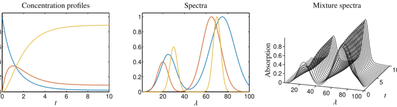
Z withκ1 = 1, κ−1=0.25,κ2=1 andκ−2=0.1. The initial concentrations arecX(0)=1,cY(0)=0 andcZ(0)=0. The concentration profiles are computed fork=101 equidistant nodes int∈[0,10] by using the MatLabode45 routine with the control parameters^RelTol=10⁻¹⁰and^AbsTol=10⁻¹⁰. The spectral profiles are sums of Gaussians

sX(λ)=0.5g(λ,25,100)+g(λ,75,250), sY(λ)=0.4g(λ,20,50)+g(λ,65,150), sZ(λ)=0.6g(λ,30,25)+g(λ,70,25) withg(λ,a,b)=exp(−(λ−a)²/b). These functions are evaluated forn =500 equidistant nodes in [1,100] in order to formS_i1 =s_X(λi),S_i2 =s_Y(λi) andS_i3 =s_Z(λi) fori=1, . . . ,n. HenceD=CS^T ∈R^101×500. Figure 4 shows all profiles and the mixture data.

7

0 20 40 60 80 100 0

0.1 0.2 0.3 0.4

0 20 40 60 80 100

0 0.05 0.1 0.15 0.2 0.25

0 1 2 3

-2 0 2 4 6

0 1 2 3

0 2 4 6 8 10

Series of spectra - component 1 Series of spectra - component 2

Series of conc. profiles - component 1 Series of conc. profiles - component 2

Figure 3: The bands of spectra and concentration profiles for the two-component model problem. The profiles within a band of solutions can only intersect within an isosbestic point due to their monotone increasing or decreasing character. The band boundaries, which are determined by the minimum and maximum of the SCF, are drawn in green and red.

4.1. The AFS and MCR-Bands profiles

The two AFS sets for the given spectral data matrix are computed by the dual Borgen plot procedure [16, 23], see also the FACPACK software [24]. The result is shown in Figure 5. The representatives of the 12 extremal profiles of the SCF (3), namely a minimum and a maximum for each of three pure component spectra and each of the associated concentration profiles, are marked in Figure 5. Points that belong to a maximum of the SCF are marked by a cross and minimum points are marked by a circle. The spectral profile that maximizes the SCF for the componentYis not located on the boundary ofMS. In order to rule out the option of a failed optimization, we analyze the behavior of the SCF below.

4.2. Analysis of the SCF

In order to confirm that the maximum of the spectral SCF for the componentY is attained in the interior of the AFS, we investigate the local behavior of the SCF (3). To this end we cover theith subset of each of the two AFS sets byNiuniformly distributed grid points and fix theith row ofT by the row vector (1,x⁽ⁱ⁾_j ), j=1, . . . ,Ni. Therein,x⁽ⁱ⁾_j are the coordinates of the jth grid point for theith component in row vector form. Then for each grid point the SCF is maximized and also minimized. The resulting function values are stored as

w⁽ⁱ⁾_j = max

T,C≥0,S≥0gi(T) with T(i,:)=(1,x⁽ⁱ⁾_j ), 3⁽ⁱ⁾

j = min

T,C≥0,S≥0gi(T) with T(i,:)=(1,x⁽ⁱ⁾_j).

The MatLaboptimization by fmincon is used; MCR-Bands works with the same routine. In order to support and stabilize the optimizations we use smart initial guesses on the basis of feasible solutions from the geometric, triangle- based Borgen plot construction. Furthermore, fmincon is started several times with different options (e.g. the interior- point-algorithm and active-set-algorithm are used each withTolX=1.E-8). The results are evaluated and the optimal results are selected. About 3% of the optimizations fail and are not plotted. The computational costs are high as 16 optimizations are started for each node.

8

0 2 4 6 8 10 0

0.2 0.4 0.6 0.8 1

t

Concentration profiles

20 40 60 80 100

0 0.2 0.4 0.6 0.8 1

λ Spectra

20 40 60 80 100 0 5

10 0

0.2 0.4 0.6 0.8

λ t

Absorption

Mixture spectra

Figure 4: The concentration profiles (left), the pure component spectra (center) and the mixture spectra (right, only every 5th spectrum is plotted) for the three-component model problem. Blue:X, red:Y, yellow:Z.

−2 0 2 4 6

−20

−15

−10

−5 0 5 10

y1

y2

AFS of the concentration factorMC

0 0.5 1 1.5

−1

−0.5 0 0.5

x1

x2

AFS of the spectral factorM_S

Figure 5: AFS plots for the model problem with colors being consistent to Figure 4. The MCR-Bands extremal profiles maximizing (×symbol) or minimizing (◦symbol) the SCF are marked by their representatives (4). The point representing the maximum of the AFS for the componentYis not located on the boundary of the AFS.

The results of these computations are plotted as two-dimensional functions P⁽ⁱ⁾_max

j=

x⁽ⁱ⁾_j ,w⁽ⁱ⁾_j

,

P⁽ⁱ⁾_min

j= x⁽ⁱ⁾_j ,3⁽ⁱ⁾

j

(19)

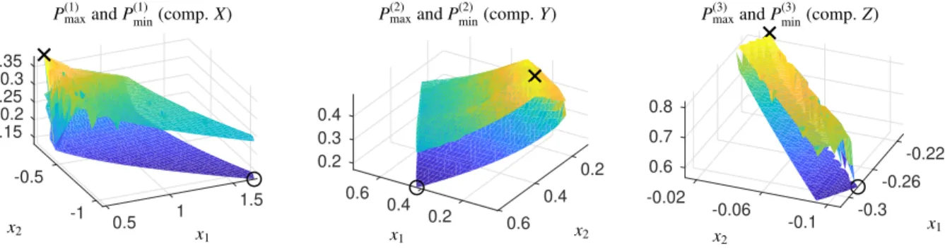
for each of the three components,i=1,2,3, and j=1, . . . ,Ni. Figure 6 shows the results withN1 =394,N2=745 andN3 =489. The minima and maxima are marked by◦respectively×. Close to the extremal solutions no outliers can be seen. This confirms the correctness of the results. The maximum point for componentY is not located on the boundary. This verifies the results from Figure 5. These results are supported by contour plots of P⁽ⁱ⁾max

andP⁽ⁱ⁾_minas shown in Figure 7. Finally, Fig. 8 shows the bands of feasible solutions together with the profiles that maximize/minimize the SCF. The coordinates of the points in the AFS that minimize or maximize the SCF and the associated values of the SCF (3) are listed in Table 1.

5. Conclusion

For two-component systems the SCF has the by no means obvious characteristic that its minimum and maximum supply the profiles that enclose the bands of all possible profiles under the nonnegativity constraint. This property of the SCF is quite surprising for the (globally) non-convex SCF function.

For systems with three or more chemical components we are not aware of publications in which SCF-maximizing or -minimizing profiles are reported to be represented by points in the AFS that are not on its boundary. Instead, these points have always been observed to be located on the boundary in a way that is known from two-component systems.

At the moment, no general analysis is known that provides conditions on the form of the spectral and concentration profiles so that the SCF attains its extrema in the interior of the AFS. However, the model problem in Section 4 together with its numerical analysis shows that the SCF for three-component systems can attain its maximum in an interior point of the AFS. We expect that our counterexample of a three-component system can be extended to systems with more chemical components in a way that the SCF-extremality on the boundary is still broken.

Summarizing, it remains to be noted that the SCF and MCR-Bands are valuable and computationally inexpensive tools for estimating the extent of rotational ambiguity underlying a chemical reaction system. The SCF provides exact bounds for the rotational ambiguity and for the bands of feasible solutions for two-component systems. For systems with three and more components the experiences, as reported in chemometric publications so far, show that the SCF-minimizing and -maximizing profiles often provide useful approximations in order to estimate the under- lying rotational ambiguity even if no feasible lower and upper feasible profiles exist that bound the full range of all

9

0.15 0.2 0.25

-0.5 0.3 0.35

1 1.5 -1 0.5

x₁ x₂

P⁽¹⁾_maxandP⁽¹⁾_min(comp.X)

0.2 0.2

0.6 0.4

0.4 0.3

0.2 0.6

0.4

x1 x2

P⁽²⁾_maxandP⁽²⁾_min(comp.Y)

-0.22 -0.26 0.6

-0.02

-0.3 -0.06

-0.1 0.7

0.8

x1

x2

P⁽³⁾_maxandP⁽³⁾_min(comp.Z)

Figure 6: Mesh plots toP⁽ⁱ⁾maxandP⁽ⁱ⁾_minby (19). Especially, the maximization of the SCF is not always successful (see the outliers). The MCR-Bands maxima are marked by×symbols, and the minima are marked by◦symbols.

0.5 1 1.5

-1 -0.8 -0.6 -0.4

x1

x2

P⁽¹⁾_min(min. comp.X)

0.2 0.4 0.6

0.2 0.3 0.4 0.5 0.6

x1

x2

P⁽²⁾_min(min. comp.Y)

-0.3 -0.25 -0.2

-0.1 -0.08 -0.06 -0.04 -0.02

x1

x2

P⁽³⁾_min(min. comp.Z)

0.5 1 1.5

-1 -0.8 -0.6 -0.4

x1

x2

P⁽¹⁾_max(max. comp.X)

0.2 0.4 0.6

0.2 0.3 0.4 0.5 0.6

x1

x2

P⁽²⁾_max(max. comp.Y)

-0.3 -0.25 -0.2

-0.1 -0.08 -0.06 -0.04 -0.02

x1

x2

P⁽³⁾max(max. comp.Z)

Figure 7: Contour plots for the surfacesP⁽ⁱ⁾_min(top) andP⁽ⁱ⁾max(bottom). The maxima and minima are marked by×respectively◦. The contour lines ofP⁽²⁾maxclearly indicate that the maximum is attained in the interior of the respective subset of the AFS.

10

Component X Component Y Component Z

x1 x2 SCF x1 x2 SCF x1 x2 SCF

Min. SCF 1.667 -1.081 0.01715 0.4214 0.6033 0.03003 -0.2851 -0.1079 0.3217 Max. SCF 0.5538 -0.2145 0.1432 0.1853 0.2279 0.24402 -0.2098 -0.02620 0.6728

Table 1: The table contains the positions and function values of the SCF extrema (minimum points◦and maximum points×) for the factorSas shown in Fig. 5.

0 5 10

0 20 40 60 80

t

Concentration profiles forX

0 5 10

0 5 10 15 20

t

Concentration profiles forY

0 5 10

0 2 4 6 8

t

Concentration profiles forZ

20 40 60 80 100

0 0.05 0.1 0.15 0.2 0.25

λ Spectral profiles forX

20 40 60 80 100

0 0.05 0.1

λ Spectral profiles forY

20 40 60 80 100

0 0.05 0.1 0.15

λ Spectral profiles forZ

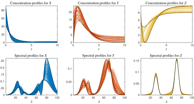
Figure 8: Bands of feasible solutions for the AFS shown in Figure 5. Upper row: feasible concentration profiles. Lower row: feasible spectral profiles. The profiles that maximize/minimize the SCF are drawn in black. The spectrum ofYthat maximizes the SCF and that is not located on the boundary of the AFS is drawn by a black broken line. The associated concentration profile is also marked by a black broken line.

feasible profiles. Nevertheless, the information that can be extracted from the theoretically deeper AFS concept can be approximated to some extent by the extrema of the SCF.

A. Mathematical background

The reducibility/irreducibility of a square matrix is defined as follows [13].

Definition A.1. Anℓ×ℓmatrix A withℓ≥2is called reducible, if anℓ×ℓpermutation matrix P exists so that PAP^T = A1,1 A1,2

0 A2,2

! .

Therein A1,1is an m×m submatrix and A1,2is an m×(ℓ−m)submatrix with1≤m< ℓ. If such a permutation matrix does not exist, then A is called an irreducible matrix. If A is a symmetric matrix, then A2,1=0implies that A1,2=0 due to the symmetry of PAP^T.

Irreducibility of a matrix is an important assumption of the Perron-Frobenius spectral theorem of nonnegative matrices [13].

Theorem A.2. Let A∈R^ℓ×ℓbe an irreducible, nonnegative matrix. Then it holds that

1. The spectral radiusρ(A), i.e., the maximum of the absolute values of the eigenvalues of A, is an eigenvalue of A.

2. For the eigenvalueρ(A)a componentwise strictly positive eigenvector exists.

3. The eigenvalueρ(A)is simple (i.e., has the multiplicity 1).

11

B. Proof of the inequalities from(14)and(16)

The inequalities (14) and (16) are equivalent. We have to prove for any column vectorsu,3 ∈ Rⁿwithkuk2 = k3k₂=1,u^T3=0 and component-wiseu>0 that

i=1,...,nmax −3_i u_i· max

j=1,...,n

3_j

u_j ≥1. (20)

A proper re-indexing of3anduallows us to assume that the negative components of3appear in the firstmcomponents of3. Then let

a_i=−3_i, i=1, . . . ,m, and b_i=3_i+m, i=1, . . . , ℓ withℓ=n−m. The lastℓcomponents ofuare taken to form the vectorw

wi=ui+m, i=1, . . . , ℓ.

Thus we can write the assumptions completely in nonnegative numbers, namely the orthogonality relation as Xm

i=1

uiai= Xℓ

j=1

wjbj

and the normalizations as

Xm

i=1

a²_i + Xℓ

j=1

b²_j=1,

Xm

i=1

u²_i + Xℓ

j=1

w²_j =1.

We have to prove that

i=1,...,mmax ai

ui

· max

j=1,...,ℓ

bj

wj

≥1.

Proof:Let

α:= max

i=1,...,m

ai

u_i and β:= max

j=1,...,ℓ

bj

w_j. Then it holds

Xm

i=1

uiai= Xm

i=1

u²_iai

ui

≤α Xm

i=1

u²_i and Xℓ

j=1

wjbj= Xℓ

j=1

w²_jbj

wj

≤β Xℓ

j=1

w²_j. Thus,

αβ=αβ





Xℓ

j=1

w²_j+ Xm

i=1

u²_i



=α



β Xℓ

j=1

w²_j



+β



α Xm

i=1

u²_i





≥α





Xℓ

j=1

wjbj



+β





Xm

i=1

uiai



=α





Xm

i=1

uiai



+β





Xℓ

j=1

wjbj





≥ Xm

i=1

a²_i + Xℓ

j=1

b²_j=1. 2

Acknowledgement

The authors are grateful to Prof. M. Tasche, University of Rostock, for his support concerning the proof of the inequality (20).

12

References

[1] P.J. Gemperline. Computation of the range of feasible solutions in self-modeling curve resolution algorithms. Anal. Chem., 71(23):5398–

5404, 1999.

[2] R. Tauler. Calculation of maximum and minimum band boundaries of feasible solutions for species profiles obtained by multivariate curve resolution.J. Chemom., 15(8):627–646, 2001.

[3] H. Abdollahi, M. Maeder, and R. Tauler. Calculation and meaning of feasible band boundaries in multivariate curve resolution of a two- component system.Anal. Chem., 81(6):2115–2122, 2009.

[4] H. Abdollahi and R. Tauler. Uniqueness and rotation ambiguities in multivariate curve resolution methods. Chemom. Intell. Lab. Syst., 108(2):100–111, 2011.

[5] R. Rajk´o. Additional knowledge for determining and interpreting feasible band boundaries in self-modeling/multivariate curve resolution of two-component systems.Anal. Chim. Acta, 661(2):129–132, 2010.

[6] W.H. Lawton and E.A. Sylvestre. Self modelling curve resolution.Technometrics, 13:617–633, 1971.

[7] O.S. Borgen and B.R. Kowalski. An extension of the multivariate component-resolution method to three components. Anal. Chim. Acta, 174:1–26, 1985.

[8] R. Rajk´o and K. Istv´an. Analytical solution for determining feasible regions of self-modeling curve resolution (SMCR) method based on computational geometry.J. Chemom., 19(8):448–463, 2005.

[9] A. Golshan, H. Abdollahi, and M. Maeder. Resolution of rotational ambiguity for three-component systems. Anal. Chem., 83(3):836–841, 2011.

[10] M. Sawall, C. Kubis, D. Selent, A. B¨orner, and K. Neymeyr. A fast polygon inflation algorithm to compute the area of feasible solutions for three-component systems. I: Concepts and applications.J. Chemom., 27:106–116, 2013.

[11] A. Golshan, H. Abdollahi, S. Beyramysoltan, M. Maeder, K. Neymeyr, R. Rajk´o, M. Sawall, and R. Tauler. A review of recent methods for the determination of ranges of feasible solutions resulting from soft modelling analyses of multivariate data. Anal. Chim. Acta, 911:1–13, 2016.

[12] M. Sawall, A. J ¨urß, H. Schr¨oder, and K. Neymeyr.On the analysis and computation of the area of feasible solutions for two-, three- and four- component systems, volume 30 of Data Handling in Science and Technology, “Resolving Spectral Mixtures”, Ed. C. Ruckebusch, chapter 5, pages 135–184. Elsevier, Cambridge, 2016.

[13] R.S. Varga.Matrix Iterative Analysis. Springer Series in Computational Mathematics. Springer Berlin Heidelberg, 1999.

[14] M. Sawall and K. Neymeyr. A fast polygon inflation algorithm to compute the area of feasible solutions for three-component systems. II:

Theoretical foundation, inverse polygon inflation, and FAC-PACK implementation.J. Chemom., 28:633–644, 2014.

[15] A. J ¨urß, M. Sawall, and K. Neymeyr. On generalized Borgen plots. I: From convex to affine combinations and applications to spectral data.

J. Chemom., 29(7):420–433, 2015.

[16] M. Sawall, A. J ¨urß, H. Schr¨oder, and K. Neymeyr. Simultaneous construction of dual Borgen plots. I: The case of noise-free data.J. Chemom., 31:e2954, 2017.

[17] M. Vosough, C. Mason, R. Tauler, M. Jalali-Heravi, and M. Maeder. On rotational ambiguity in model-free analyses of multivariate data.J.

Chemom., 20(6-7):302–310, 2006.

[18] A. Golshan, M. Maeder, and H. Abdollahi. Determination and visualization of rotational ambiguity in four-component systems.Anal. Chim.

Acta, 796(0):20–26, 2013.

[19] M. Sawall and K. Neymeyr. A ray casting method for the computation of the area of feasible solutions for multicomponent systems: Theory, applications and FACPACK-implementation. Anal. Chim. Acta, 960:40–52, 2017.

[20] M. Sawall, H. Schr¨oder, D. Meinhardt, and K. Neymeyr. On the ambiguity underlying multivariate curve resolution methods. In R. Tauler, editor,Comprehensive Chemometrics, 2nd edition, page To be published. Elsevier, 2019.

[21] J. Jaumot and R. Tauler. MCR-BANDS: A user friendly MATLAB program for the evaluation of rotation ambiguities in multivariate curve resolution.Chemom. Intell. Lab. Syst., 103(2):96–107, 2010.

[22] R. Rajk´o. Computation of the range (band boundaries) of feasible solutions and measure of the rotational ambiguity in self- modeling/multivariate curve resolution.Anal. Chim. Acta, 645(1–2):18–24, 2009.

[23] M. Sawall, A. Moog, C. Kubis, H. Schr¨oder, D. Selent, R. Franke, A. Br¨acher, A. B¨orner, and K. Neymeyr. Simultaneous construction of dual Borgen plots. II: Algorithmic enhancement for applications to noisy spectral data.J. Chemom., 32:e3012, 2018.

[24] M. Sawall, A. Moog, and K. Neymeyr. FACPACK: A software for the computation of multi-component factorizations and the area of feasible solutions, Revision 1.3. FACPACK homepage: http://www.math.uni-rostock.de/facpack/, 2018.

13