On the area of feasible solutions and its reduction by the complementarity theorem

(1)

On the area of feasible solutions

and its reduction by the complementarity theorem

Mathias Sawall^a, Klaus Neymeyr^a,b

aUniversit¨at Rostock, Institut f¨ur Mathematik, Ulmenstrasse 69, 18057 Rostock, Germany.

bLeibniz-Institut f¨ur Katalyse, Albert-Einstein-Strasse 29a, 18059 Rostock, Germany.

Abstract

Multivariate curve resolution techniques in chemometrics allow to uncover the pure component information of mixed spectroscopic data. However, the so-called rotational ambiguity is a difficult hurdle in solving this factorization problem. The aim of this paper is to combine two powerful methodological approaches in order to solve the factorization problem successfully. The first approach is the simultaneous representation of all feasible nonnegative solutions in the area of feasible solutions (AFS) and the second approach is the complementarity theorem. This theorem allows to formulate serious restrictions on the factors under partial knowledge of certain pure component spectra or pure component concentration profiles.

In this paper the mathematical background of the AFS and of the complementarity theorem is introduced, their mathematical connection is analyzed and the results are applied to spectroscopic data. We consider a three-component reaction subsystem of the Rhodium-catalyzed hydroformylation process and a four-component model problem.

Key words: spectral recovery, multivariate curve resolution, nonnegative matrix factorization, area of feasible solutions, complementarity theorem.

1. Introduction

Multivariate curve resolution (MCR) methods in chemometrics are important and successful tools to extract information on the pure components from spectroscopic data of multi-component chemical reaction systems. However, MCR methods suffer from the so-called rotational ambiguity. This means that the factorization problem for the spectral data matrix often has wide ranges of nonnegative solutions. These solutions are called feasible factors. From these solutions the “true”

nonnegative concentration profiles of the pure components and their associated spectra are to be selected. For two-component systems the observation of such continua of possible solutions has been made by Lawton and Sylvestre [1]. They also gave a representation of these continua of solutions by plotting the associated expansion coefficients in the plane. Such a representation of range of feasible solutions by sets of expansion coefficients is called an area of feasible solutions (AFS).

For three-component systems Borgen and Kowalski [2]

have devised a technique for representing the AFS also in the two-dimensional plane. For details on the construction of the AFS see [3, 4, 5, 6]. The numerical

computation of the AFS is very intensive in terms of computing time. For three-component systems efficient numerical processes have been presented in [7, 8, 9].

For four-component systems Golshan, Maeder and Ab- dollahi [10] recently presented a technique to compute the AFS.

1.1. Using supplemental information

Once having computed the AFS for a given spectral data matrix, one is interested in selecting one solution from the AFS which fits best the chemical system under consideration. Any further information on the reaction system can help to decrease the ambiguity and so to reduce the AFS. Various chemometric techniques have been developed to this end. Examples are the window factor analysis [11], the evolving factor analysis [12, 13], the application of unimodality conditions [14]

or the use of kinetic models [15, 16, 17, 18] and last but not least the uniqueness theorems by Manne [19]. An- other approach for feeding-in partial knowledge of the factors in order to reduce the rotational ambiguity is the complementarity and coupling theory which have been introduced in [20].

... April 29, 2014

(2)

1.2. Aim and organization of this paper

The aim of this paper is to combine the complementarity theorem from [20] with the AFS for systems with an arbitrary number of components; practical applica- tions are shown for three- and four-component chemical reaction systems. It is shown how the knowledge of a single spectrum, i.e. a single point of the spectral AFS, can reduce the AFS for the concentration factor for the remaining components to a straight line in case of a three-component system and vice versa, cf. [21, 9].

We also consider four-component systems where a pre- given point in the spectral AFS results in a plane in the AFS for the concentration factors. Such additional information on a chemical reaction system is sometimes accessible as the spectra of the reactants or the spectrum of the main product might be available. In other cases there are techniques to determine the concentration profiles of certain species. In Section 4 we consider exper- imental data from the Rhodium-catalyzed hydroformylation from which a catalytic subsystem with three components is studied.

The paper is organized as follows: After a brief introduction to the spectral recovery problem and to the AFS, the mathematical background for the application of the complementarity theorem to the AFS is discussed in Section 3. Numerical results are presented for a three-component system which is a subsystem of the Rhodium-catalyzed hydroformylation. Further a four- component model problem is studied.

2. Area of feasible solutions 2.1. The factorization problem

The key equation for the following analysis is the low-rank-approximation of the spectral data matrix D∈ R^k×n

D≈UΣT⁻¹

| {z }

C

T V^T

|{z}

A

, (1)

which can be computed from a singular value decompo- sition [22] of D. Therein U is a k×s matrix containing the first s left singular vectors of D, the n×s matrix V contains the first s right singular vectors of D andΣ is the s×s diagonal matrix with the s largest singu- lar values on its diagonal, see [23, 24] for details. The regular s×s matrix T serves to represent the rotational ambiguity. The desired approximate factors C and A of D can be computed by right-multiplication of UΣwith T⁻¹and left multiplication of V^Tby T . Spectral recov- ery amounts to the construction of a suitable T by using

soft constraints, kinetic models or any other additional information, see e.g. [15, 16, 14, 25, 26].

A systematic and fundamental approach to the factorization problem is to compute and to represent the full set of all nonnegative solutions simultaneously. This complete representation is just the AFS. For an expla- nation of the AFS see the seminal papers of Borgen and Kowalski [2] as well as Rajk ´o and Istv´an [3]. Newer contributions on the numerical computation of the AFS for two-, three- and four-component systems can be found in [5, 7, 8, 9, 10].

2.2. Singular vector expansions

The representation of the AFS for the spectral factor is based on the expansion of the spectra with respect to the basis of right singular vectors given by V. In a similar way the AFS for the concentration factor rests on an expansion of the concentration profiles with respect to the basis of left singular vectors given by U.

In (1) the rows (spectra) of A are represented as linear combinations of the right singular vectors, which are the columns of V. The ith row of A=T V^T reads

A(i,:)=(ti1, . . . ,tis)V^T =ti1

1,ti2

ti1

, . . . ,tis

ti1

| {z }

=:x

V^T

=ti1(1,x)V^T.

(2)

Therein ti1 , 0 has been used, a fact which is by no means obvious, but has been proved in Theorem 2.2 of [9]. Equation (2) shows that the ith spectrum A(i,:) aside from scaling is uniquely determined by the row vector x ∈ R^s−1of expansion coefficients. The scaling constant ti1in (2) can be written as

ti1=(T )i1=(AV)i1=(AV(:,1))i. (3)

The construction for the factor C is similar. The jth column of C =UΣT⁻¹with (T⁻¹)i j=¯ti jreads

C(:,j)=UΣ(¯t1 j, . . . ,¯ts j)^T

=¯t1 jUΣ 1,¯t2 j

¯t1 j

, . . . ,¯ts j

¯t1 j

| {z }

=:y

T

=¯t1 jUΣ(1,y)^T.

(4)

Once again, ¯t1 j,0 is guaranteed by Theorem 2.2 in [9].

It holds that

¯t1 j=(T⁻¹)1 j=(Σ⁻¹U^TC)1 j=σ⁻¹₁ U(:,1)^TC(:,j). (5) 2

(3)

2.3. The AFS

As shown in Equation (2) any spectrum can be repre- sented (aside from scaling) by its vector x of expansion coefficients with respect to the right singular vectors V(:,2), . . . ,V(:,s). This is the basis for a low dimen- sional representation of the AFS. A further argument is needed for the representation of the AFS, namely that by a permutation matrix P and its inverse P^Tcan be in- serted between C and A in (1) and that this allows to rearrange the row of A and columns of C arbitrarily, since CA =(CP^T)(PA) =(UΣT⁻¹P^T)(PT V^T). There- fore only the first row of T is to be considered in order to define the AFS for the spectral factor. The delineation of the area of feasible solutions (AFS) under nonnegativity constraints for an s-component system is as follows

M_A={x∈R^s−1 : exists invertible T ∈R^s×s, T (1,:)=(1,x), UΣT⁻¹≥0 and T V^T ≥0}.

(6) For a two-component system (s=2) the AFS is a real interval, for a three-component system (s = 3) it is a subset in the plane and for s=4 it is a subset of theR³. For s=2 the interval-AFS can easily be written down explicitly. For s =3 geometric approaches to the construction of the AFS can be found in [2, 3]. Numerical methods for the computation of the AFS for s=2,3,4 are described in [5, 7, 10, 8, 9].

In a similar manner the AFSM_C for the concentration factor can be defined. According to (4) and with the same arguments used above, matrices Z are to be deter- mined with the first row equal to (1, . . . ,1) ∈ R^s and with Z(:,1)^T =(1,y) for y∈R^sso that UΣZ and Z⁻¹V^T are nonnegative matrices.

In short formMAandMCare given by M_A:={x∈R^s−1: UΣT⁻¹≥0 and T V^T ≥0}

MC:={y∈R^s−1: UΣZ≥0 and Z⁻¹V^T ≥0} (7) with invertible s×s matrices T and Z so that

T (1,:)=(1,x), Z(:,1)^T =(1,y)

and every matrix element of the first column of T and the first row of Z equals 1. For general data D the matri- ces T and Z⁻¹ do not coincide since the restrictions on T and Z cannot be fulfilled simultaneously.

2.4. Block representation

For this paper it is useful to represent C and A and some of their submatrices by their expansion coeffi- cients x and y according to (2) and (4). We call this the block representation of truncated expansion coefficients with respect to the basis of singular vectors.

Definition 2.1. Let s0 be an integer with 1 ≤ s0 ≤ s and let for i = 1, . . . ,s0 the row vector x⁽ⁱ⁾ ∈ R^s−1 be the truncated vector of expansion coefficients of A(i,:) with respect to the right singular vectors in the sense of (2). Considering s0 rows of A(1 : s0,:) simultaneously yields

X=





 x⁽¹⁾

... x^(s⁰⁾







∈R^s⁰^×(s−1)

as the block representation of truncated expansion co- efficients.

In the same way let y^{( j)}be the representative of C(:,j) in the sense of (4). Then

Y=





 y⁽¹⁾

... y^(s⁰⁾







∈R^s⁰^×(s−1)

is the block representation of C(:,1 : s0).

Remark 2.2. If s0 = s, then the block representations X,Y ∈ R^s×(s−1)define two simplices in theR^s−1 whose vertices are the row vectors of either X or Y.

Further, Equations (2) and (3) result in A(i,:)=(AV(:,1)i(1,x⁽ⁱ⁾))V^T.

This yields for s0 = s and with the s-dimensional 1- vector e=(1, . . . ,1)^T ∈R^s

A=M₁(e,X)V^Twith M₁=diag(AV(:,1)).

Similarly, Equations (4) and (5) result in C(:,j)=(σ⁻¹₁ U(:,1)^TC(:,j)) UΣ(1,y^{( j)})^T so that for s0=s

C=UΣ e^T Y^T

!

M2with M2=diag(σ⁻¹₁ U(:,1)^TC).

3. The AFS and the complementarity theorem As stated in Section 1.1 there are various techniques how to feed in partial knowledge of the factors in order to reduce the rotational ambiguity of an MCR method.

Here we would like to show how the complementarity theorem from [20] can be applied for the purpose of a reduction of the AFS.

3

(4)

−0.5 0 0.5

−0.8

−0.6

−0.4

−0.2 0 0.2 0.4

Series of feasible points inMA

α=x1

β=x2

−2 −1 0 1 2

−10 0 10 20

Associated straight lines inMC

α=x1

β=x2

2000 2050 2100

0 0.05 0.1 0.15

Series of spectra

wavelength [1/cm]

Figure 1: Application of Theorem 3.1 to an (s=3)-component system for the Rhodium-catalyzed hydroformylation process, see Section 4.1 or [27] for details. Left: the spectral AFS is contoured by black lines and consists of three separated segments. A series of feasible spectra is shown by single points colored from blue to red. Right: the series of spectra which are associated with the series of points inMA. Center: Set of straight lines or one-dimensional affine subspaces inMCwhich are associated with the points inMAand which are shown in the same coloration. The axes of the AFS plots are x1and x2. For a three-component system these axes equal (α, β) according to the standard notation.

3.1. Mutual reduction ofM_C andM_A by the comple- mentarity theorem

The complementarity theorem from [9] shows how pre-given spectra for certain pure components restrict the concentration profiles for the remaining components and vice versa. A comparable observation has been made in [21] for three-component systems.

For a reproduction of the complementarity theorem in concise form see Appendix 6.1. Next it is shown how such a pre-given spectrum, which is represented by a single point in the spectral AFSMA reduces the AFS MCfor the complementary components.

Theorem 3.1. Let a spectrum/row A(i₀,:) be given. Ac- cording to (2) it holds A(i₀,:)=t_i₀₁(1,x)V^T and x spec- ifies a point in the spectral AFSMA.

Then all concentration profiles C(:,j) with j,i₀are represented in the sense of (4) by points y which are elements of the s−2-dimensional affine subspace

C⁽ⁱ⁰⁾=









y∈R^s−1: Xs−1

ℓ=1

xℓyℓ =−1









. (8)

Thus all feasible concentration profiles C(:,j) with j, i₀have the form

UΣ(1,y)^T with y∈ C⁽ⁱ⁰⁾.

Proof. For given A(i0,:) Theorem 4.2 from [20], see also Appendix 6.1, can be applied (for the case that 1 : s0 is substituted by i0). This theorem guarantees that the complementary concentration profiles C(:,j) for

j,i0are elements of the space

{UΣ˜y : for ˜y∈R^swith A(i0,:)V ˜y=0}. (9)

Therein ˜y is a column vector in theR^s.

Insertion of A(i0,:)=ti₀1(1,x)V^T into (9) shows that ti₀1(1,x)V^TV ˜y=ti₀1(1,x)˜y=0 (10) is the decisive condition, which is now transformed in order to prove (8). First, Equation (4) allows to write the concentration profile C(:,j)=UΣ˜y in the form

UΣ˜y=¯t1 jUΣ(1,y)^T

with the row vector y ∈ R^s−1. Thus ˜y = ¯t1 j(1,y)^T. In- serting this into (10) yields

ti01¯t1 j(1,x) (1,y)^T=ti01¯t1 j

1+ Xs−1

ℓ=1

xℓyℓ

=0.

Since ti₀1¯t1 j , 0, the second factor equals 0, i.e.Ps−1

ℓ=1xℓyℓ =−1, which proves (8).

Finally, the dimension ofC⁽ⁱ⁰⁾equals s−2 because the vector y∈R^s−1has to satisfy one linear constraint.

The setC⁽ⁱ⁰⁾is an (s−2)-dimensional affine subspace which is a hyperplane inR^s−1and which intersectsM_C. Further, Theorem 3.1 also applies to the situation in whichMAandMChave changed their places. This fact does not require a separate proof but is now stated explicitly.

Corollary 3.2. Theorem 3.1 is applicable to the case in which A and C are swapped. Then a given representa- tive y for a concentration profile C(:,i₀) results in the set

A⁽ⁱ⁰⁾=









x∈R^s−1: x·y^T = Xs−1

ℓ=1

xℓyℓ =−1









of representatives for the complementary pure compo- nent spectra A( j,:) with j,i0.

4

(5)

Theorem 3.1 constitutes a relation between a certain point in either the spectral or concentrational AFS with an affine subspace in the concentrational or spectral AFS. For a two-component system a certain point x∈ MA is directly related with another point y∈ MC. For a three-component system a certain point x ∈ MA

is connected with a straight line inMC, see also [21, 9].

This is demonstrated in Figure 1 where for the case s = 3 a series of feasible points in MA is shown together with the set of associated one-dimensional affine subspaces (straight lines). Details on this problem are presented in Section 4.1. For an (s = 4)-component system a certain point x ∈ M_A is related with a plane;

this is demonstrated in Section 4.2 for a model problem.

If more than one spectrum or concentration profile of the pure components is known, thenM_AandM_Ccan be further reduced. Then, in the best case, even a unique decomposition can be determined.

Corollary 3.3. For given s₀rows A(i,:), i= 1, . . . ,s₀, let x⁽ⁱ⁾∈R^s−1be the representatives in the sense of (2).

Let X ∈ R^s⁰^×(s−1)be the block representation of these coefficients according to Definition 2.1.

Then the representatives y∈ MC of the complemen- tary columns C(:,j), j= s0+1, . . . ,s, are elements of the (s−s0−1)-dimensional affine subspace

C^(1:s⁰⁾=n

y∈R^s−1: Xy^T =(−1, . . . ,−1)^To

. (11)

Proof. Let C(:,j) with j > s0 be a concentration pro- file and let y ∈ M_Cbe its representative, see Equation (4). Theorem 3.1 imposes the conditions x⁽ⁱ⁾y=−1 for i=1, . . . ,s₀, which gives (11). The dimension ofC^(1:s⁰⁾ equals s−s₀−1 since s₀ linear equations are imposed on y∈R^s−1.

Remark 3.4. The dimension s−s0−1 ofC^(1:s⁰⁾is consis- tent with the dimension s−s0in Equation (7) of Theorem 4.2 in [20]. The reason that the dimension ofC^(1:s⁰⁾is reduced by 1 is that the block representation of the ex- pansion coefficients in Definition 2.1 includes the fixed scaling of the first left singular vector. In other words, (1,y) is the vector of expansion coefficients under scal- ing assumptions andω(1,y), forω∈R, is the full sub- space without any scaling.

Corollary 3.3 can also be formulated in a way in which C and A have changed their places.

3.2. Simplices inM_CandM_Aand their relations In this section we assume that so much information on a factor is available that the second factor is completely determined by the complementarity theorem. A well known fact on MCR factorizations D=CA is that

one given factor determines the second factor. The second factor can be determined as follows: In the case of noise-free data D a linear system of equations is to be solved if CA has the full rank of D. In the case of noisy data or if a low-rank approximation of D is considered, then the second factor can be computed by solving least- squares problems. In any case the knowledge of a full factor completely determines the system.

A successful factorization means that in the AFSMA

and the AFS MC each s points are specified. These points are the vertices of two simplices, one inMAand one in MC. For the factor A the simplex in MA has the vertices x⁽ⁱ⁾, i=1, . . . ,s, see (2). The block repre- sentation of these vertices is X ∈ R^s×(s−1)according to Remark 2.2. Analogously, the factor C defines a sim- plex inM_C with the vertices y^{( j)} given by the rows of Y.

For a two-component system the simplex in Ris a line segment. For a three-component system the simplex inR²is a triangle and its edges are determined by the complementarity theorem 3.1. For four-components systems the simplex inR³ is a tetrahedron and its side surfaces, the triangles, are determined by the complementarity theorem once again. All this is analyzed and demonstrated in the following. First the relation of the simplex defined by X to the simplex defined by Y is de- scribed in Theorem 3.5.

Theorem 3.5. Let X ∈ R^s×(s−1)be the block represen- tation of A as introduced in Definition 2.1. Then the vertices Y( j,:), j =1, . . . ,s, can be computed by solv- ing s linear systems of equations. For j =1, . . . ,s and Y( j,:)=y^{( j)}the linear system of equations reads





 x⁽¹⁾

... x^{( j−1)} x^{( j+1)}

... x^(s)





 y^{( j)}T

=







−1 ...

−1







. (12)

The assertion also holds if X and Y are interchanged.

Proof. Corollary 3.3 for s0 = s −1 results in a 0- dimensional affine subspace C^(1:s−1) which is just the single vertex Y(s,:) = y^(s) and proves the case j = s.

The argument can also be applied for the remaining in- dexes j.

Theorem 3.5 and the simplices inM_A andM_C are illustrated by Figure 2 for a three-component system.

Then the axes of the AFS plots are denoted byα = x1

5

(6)

andβ=x2according to the standard notation. For details on the underlying factorization problem see Sec- tion 4.1.2.

Remark 3.6. Theorem 3.5 in Equation (12) formulates a relation between the simplices inM_CandM_Awhich are defined by X and Y. This relation cannot imme- diately be translated to a factorization of D since the feasible factorizations

D=UΣT⁻¹

| {z }

C

T V^T

|{z}

A

= UΣZ

|{z}

C^′

Z⁻¹V^T

| {z }

A^′

with T and Z defined in (7) include a specific scaling of the rows of A and columns of C. Thus in general C^′A=UΣZT V^T ,D holds. What is needed for a cor- rect representation of the factorization are the two di- agonal matrices M1 and M2 as introduced in Remark 2.2. With these matrices and with T = (e,X) and Z^T = (e,Y) for e = (1, . . . ,1)^T ∈ R^s it holds that D=UΣZ M₂M₁T V^T.

3.3. FAC-PACKimplementation

In [9] a fast numerical procedure has been introduced for the numerical computation of the AFSM_Cand the AFS M_A by the polygon inflation algorithm. A tuto- rial and the software, which is calledFAC-PACKand which is written in C with a MatLab graphical user in- terface, are available from

http://www.math.uni-rostock.de/facpack/

The first revision FAC-PACK 1.0 serves to compute the spectral AFSM_Aand the concentrational AFSM_C. The areas of feasible solutions which are shown in Fig- ures 1 and 2 have been computed withFAC-PACK. In the first quarter of 2014 the revision 1.1 ofFAC-PACK has been made publically available. This revision includes an algorithmic implementation of the complementarity theorem which allows to import known spectra or known concentration profiles, to mark their representatives in the AFS and to construct as well as to draw the complementary affine spaces. All the images shown in Figure 2 have been generated with the revision 1.1 of FAC-PACK.

3.4. A sensitivity measure with respect to noise Theorem 3.1 and Equation (8) can be used to derive a relation on the sensitivity of the AFS with respect to noise.

Lemma 3.7. Let x ∈ MA be given and let y ∈ MC

be in the complementary space of concentration profiles

as given by (8). If the perturbation of x due to noise is given byδx, then the induced perturbationδyof y is bounded as follows

kδyk ≥ |(δx)y^T|

kxk (13)

if the quadratic term (δx)(δy)^Tis ignored. The inequality also holds with (x, δ_x) and (y, δ_y) having changed their positions.

Proof. Let a certain spectrum be given and let its repre- sentative be x ∈ M_A. Theorem 3.1 shows that the rep- resentatives y of the complementary concentration pro- files fulfill xy^T =−1. Letδx ∈ R^s−1be a perturbation (row) vector of x andδybe the resulting perturbation for y. From

(x+δx)(y+δy)^T =−1 one gets after subtraction of xy^T =−1

(δx) y^T+x(δy)^T =−(δ_x)(δy)^T =O(kδ_xk kδ_yk) whereOis the Landau symbol and wherek · kis the Eu- clidean vector norm. (The Landau or big O notation is used to describe the asymptotic behavior of a function;

here it expresses that (δx)(δy)^Tis a mixed quadratic term in theδ-perturbations, which quadratically tends to 0, if δ_x→0 andδ_y→0.)

Next the second order term of perturbations on the right-hand side is ignored. Application of the Cauchy- Schwarz inequality leads to

kxk kδ_yk ≥ |x(δ_y)^T|=|(δ_x)y^T|.

This proves thatkδ_yk ≥ |(δ_x)y^T|/kxk.

Inequality (13) shows that the resulting perturbation kδykis bounded from below by|(δx)y^T|/kxk. This lower bound is reciprocal to kxkwhich is the Euclidean dis- tance of x to the origin. An interpretation of this result is as follows: For points x far away from the origin the influence of perturbationsδxon y decreases. However, any x close to the origin appears to be sensitive with respect to perturbations.

This perturbation argument is consistent with spectroscopic observations: For IR-spectra with narrow lo- calized peaks next to non-absorbing frequency bands, the representatives x are often far away from the origin.

Hence the sensitivity with respect to noisy data is rela- tively small. In contrast to this UV/Vis data often has wide absorbing frequency bands without non-absorbing bands. Then the representing vectors x of the true solu- tions are often close to the origin and the reliability of the results of Theorem 3.1 for noisy data decreases.

6

(7)

2000 2050 2100 0

0.05 0.1 0.15

actor

One given spectrum A(1,:)

wavenumber [1/cm]

unscaledabsorption

olefin

2000 2050 2100

0 0.05 0.1 0.15

Two given spectra A(1 : 2,:)

wavenumber [1/cm]

unscaledabsorption

olefin acyl complex

2000 2050 2100

0 0.05 0.1 0.15

Three given spectra A(1 : 3,:)

wavenumber [1/cm]

unscaledabsorption

olefin acyl complex hydrido complex

−0.5 0 0.5 1

−0.8

−0.6

−0.4

−0.2 0 0.2 0.4

α

β

AFSMA- one given component

−0.5 0 0.5 1

−0.8

−0.6

−0.4

−0.2 0 0.2 0.4

α

β

AFSMA- two given components

−0.5 0 0.5 1

−0.8

−0.6

−0.4

−0.2 0 0.2 0.4

α

β

AFSMA- all components known

−3 −2 −1 0 1 2 3

−10 0 10 20

α

β

AFSMC- one 1D affine space

−3 −2 −1 0 1 2 3

−10 0 10 20

α

β

AFSMC- two 1D affine spaces

−3 −2 −1 0 1 2 3

−10 0 10 20

α

β

AFSMC- all components fixed

0 200 400 600 800 1000 0

0.5 1 1.5 2

Feasible solutions C(:,2) and C(:,3)

time [min]

unscaledconcentration

0 200 400 600 800 1000 0

0.5 1 1.5 2

Feasible solutions C(:,1) and C(:,2)

time [min]

0 200 400 600 800 1000 0

0.5 1 1.5 2

Unique concentration factor

time [min]

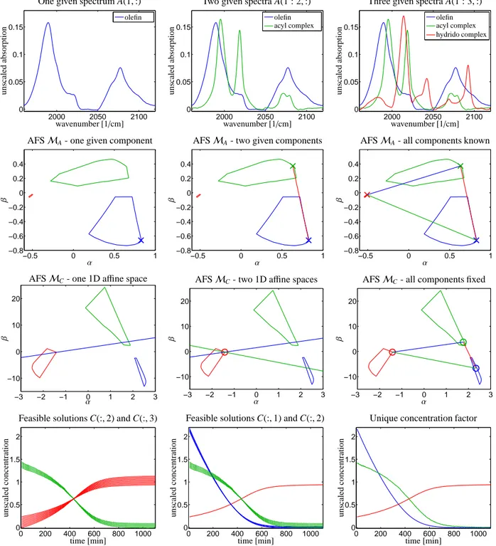
Figure 2: Application of Theorem 3.5 and Corollary 3.3 to spectral data from the Rhodium-catalyzed hydroformylation process, see Section 4.1.

Left Column: One given spectrum fixes a point inMA and a straight line inMCfor the complementary components. This results in one- dimensional continua of concentrations profiles. Center column: Two given spectra determine two points inMAand two straight lines inMC. Their intersection uniquely determines the concentration profile of the third component. Right column: Three given spectra completely determine the complete solution. The two simplices (triangles) inMAandMCaccording to Theorem 3.5 are also shown.

First row: Given one, two and three spectra (rows of A). Second row: AFSM_Awith one, two and three fixed points representing the given spectra.

Third row: AFSMCwith the affine subspaces according to Theorem 3.1 shown by one, two and three straight lines. The points of intersection of these lines uniquely determine concentration profiles. Fourth row: Series of concentration profiles which can be found in the intersection of the AFS with the affine subspaces (straight lines) according to Theorem 3.1.

Known points inMAare marked by×and are related with the straight lines inMC. Uniquely determined points inMCare marked by◦and are associated with the edges of the triangle inMA. The same coloration is used for points in eitherMAorMCand their associated line segments in eitherM_CorM_A. A rescaling of the columns of C or rows of A is necessary for a correct reconstruction D7 =CA, cf. Remark 3.6.

(8)

.

. .

x x+δx

−_kxk^x2

−_kx+δ^x+δ^x

xk²

C_y

C_y+δ_y ϕ

ϕ

Figure 3: The geometric construction underlying Lemma 3.8.

The reciprocal relation betweenkxkand the perturba- tionkδ_y||which is expressed by Equation (13) has some structural resemblance to the observation of Windig, Keenan et. al. [28] namely that in MCR techniques high contrast solutions in the C-space are related to low con- trast solutions in the A-space and vice versa.

The next lemma shows that the acute angle which is enclosed by x and x+δ_xin the A-space equals the acute angle which is enclosed by the associated one- dimensional affine spaces in the C-space and vice versa.

This result can be interpreted as a bound on the poten- tial perturbationδyresulting from a given perturbation δx. The application of this result to the AFS plots in the current paper requires that theαandβaxes are scaled to the same length units.

Lemma 3.8. For (s = 3)-component system let x and x+δxbe given inM_A. Further, letC_yandC_y+δ_y be the associated one-dimensional affine linear subspaces as determined by Theorem 3.1. Then it holds that

∡(x,x+δx)=∡(C_y,C_y+δ_y).

The relation also holds if x and y interchange their po- sitions.

Proof. For a given x inM_A any element y of the com- plementary spaceCysatisfies (x,y)=x1y1+x2y2=−1.

This relation can be rewritten in the Hesse normal form of a straight line

− x kxk,y

= + 1 kxk.

This means that theC_yis a straight line which is orthogonal to−x/kxkand whose smallest distance to the origin is 1/kxk.

Similarly the relation (x+δx,y+δy) = −1 can be rewritten as

− x+δ_x kx+δxk,y+δy

= + 1 kx+δxk

so that Cy+δ_y is a straight line which is orthogonal to

−(x+δx)/kx+δxkand whose smallest distance to the origin is 1/kx+δxk. The geometric setup is shown in Figure 3. Simple geometric arguments (on the sum of angles in a triangle) show that the acute angleϕwhich is enclosed by x and x+δxequals the acute angle enclosed byC_yandC_y+δ_y.

3.5. Further AFS reduction effects

The complementarity theory is only one source for an AFS reduction from pre-given information. Next, three different sources for a reduction of the AFS are listed.

We always assume that a single spectrum is known, i.e. a single point in the AFSM_A is determined. (The same arguments apply if a single concentration profile or single point in the AFS M_C is given.) Then, without claiming completeness, three different sources for restrictions onM_AandM_Care:

1. Restrictions on the AFS segments of the complementary components inM_C. These restrictions are the topic of the present paper.

2. Restrictions on the concentration profile of the component for which the spectrum is given.

3. Restrictions on the AFS segments for the remaining components inM_A.

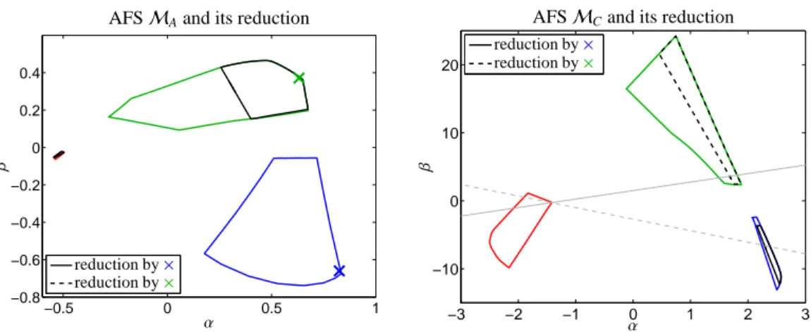
The restrictions of the AFS due to the items 2 and 3 are presented in Figure 4 for the Rhodium-catalyzed hydroformylation process, see Section 4.1. Whilst item 1 enforces a restriction to a one-dimensional affine subspace, items 2 and 3 amount to a moderate decrease of the area of the AFS segments. Further details on item 3 are contained in [9]; the AFS restrictions related to item 2 will be explained in a forthcoming paper. In any case the predictions forM_Cby the complementarity theorem are much more restrictive compared to the other criteria.

3.6. Ambiguity reduction in MCR techniques

There are various further options for the reduction of the rotational ambiguity in multivariate curve resolution techniques. For instance hard-modeling by means of a kinetic model and the restrictions on the concentration profiles in C have been presented in [16]. Other im- portant and well established techniques for the ambiguity reduction are the evolving factor analysis (EFA) and 8

(9)

−0.5 0 0.5 1

−0.8

−0.6

−0.4

−0.2 0 0.2 0.4

AFSM_Aand its reduction

reduction by× reduction by×

α

β

−3 −2 −1 0 1 2 3

−10 0 10 20

AFSMCand its reduction reduction by×

reduction by×

α

β

Figure 4: The AFS and its reduction for the spectral data from the hydroformylation process as considered in Figure 2. One or two points are fixed inMAand are marked by×and×inMA. The resulting reduced AFS segments are shown by a black solid line if only the point×is given and by a broken line if only the point×is given. In the left plot the broken line is contained in the small red segment.

The restrictions by the complementarity theorem inMCare shown by two gray straight lines. These latter predictions are very restrictive since the intersection of the two straight lines determines one point in the red segment uniquely and the intersections with the green and the blue AFS segments are short line segments.

window factor analysis (WFA) [13, 12, 11] and techniques which exploit local rank information in order to extract single pure component spectra and single concentration profiles. For these techniques the Manne theorems are key tools [19].

It is worth noting that the complementarity theory is a hard constraint due to known spectra and concentration profiles which makes predictions on the remaining unknown parts of C and A. In this sense EFA and WFA are related to the complementarity theory. However, in this paper the focus is on the AFS and additional information, which may originate from a local rank analysis, is used in order to reduce the AFS for complementary components.

4. Numerical results

For the numerical experiments we consider a series of FT/IR spectra for a reactive subsystem of the Rhodium- catalyzed hydroformylation process with three components. We also treat a model problem with four components.

4.1. Rhodium-catalyzed hydroformylation

The first application is the Rhodium-catalyzed hydroformylation process. See [27, 8] for details on the reactive subsystem consisting of the olefin, the hydrido com- plex and the acyl complex. A total number of k=1045 spectra have been used within a wavenumber interval with n=664 channels. Hence D is a 1045×664 matrix.

The spectral AFSMAis shown in Figures 1 and 2. The

concentrational AFSMC is plotted in the third row of Figure 2. For this three-component system the standard notationα=x1andβ=x2is used.

4.1.1. Series of feasible points

We start with a demonstration of the relation of points inM_Aand one-dimensional affine subspaces inM_C as proved in Theorem 3.1. Figure 1 shows a series x⁽ⁱ⁾, i = 1, . . . ,15, of 15 feasible points in one segment of MA. If we assign to this segment of the AFS the component number 1, then the complementarity theorem says that the concentration profiles C(:,2 : 3) are restricted to 1D affine subspaces inM_C. For a fixed x=x⁽ⁱ⁾the associated affine subspace isC⁽ⁱ⁾and is given by (8). Figure 1 shows that the series of points in M_A is associated with a series of 1D affine subspaces inM_C. The dimen- sion of each of these subspaces equals 1 since s=3 and only s0 = 1 spectrum is given. The associated series of spectra is also shown in Figure 1. A coloration from blue to red is used for the series of points inM_A, for the associated 1D affine subspaces inM_Cand for the series of spectra.

4.1.2. Successive reduction of the rotational ambiguity Next Theorems 3.1 and 3.5 are applied in order to demonstrate the successive reduction of the rotational ambiguity for a three-component system. The effect of supplying additional information on the factors and the resulting predictions by the complementarity theorem is monitored inMAandMCsimultaneously. Figure 2 shows all results. In the first row of this figure either 9

(10)

0 50 100 0

0.5 1

Factor C

t ⁰ ⁵⁰ ¹⁰⁰

0 0.5 1

Factor A

x

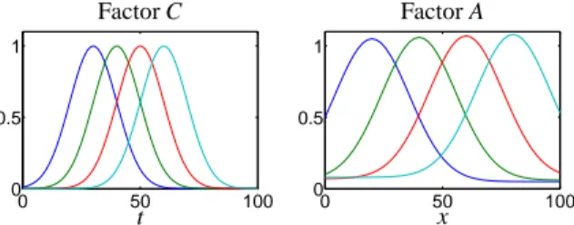
Figure 5: Four concentration profiles C ∈R^70×4 and the associated spectra A∈R^4×51of the simulated four-component model problem in Section 4.2.

one, two or three of the spectra are given. The second row shows the spectral AFS for the system with either one, two or three marked points which represent the given spectra. The third row shows the associated 1D affine subspaces in the concentrational AFS. If one spectrum is given, then the concentration profiles of the complementary components are restricted to a 1D affine space. If two spectra are given, then the concentration profile of one component is uniquely determined and for the remaining two components the concentration profiles are restricted to 1D spaces. If all three spectra are known, then all factors are uniquely determined. This situation is visualized in the right column of images in Figure 2. For this case two triangles (2D simplices) are shown inMA andMC according to Theorem 3.5. For all computations revision 1.1 of FAC-PACK has been used, see Section 3.3.

4.2. A four-component model problem

The representation of an AFS by Equation (7) as well as the arguments of the complementarity theorem from Section 3 apply to any number of components s ≥ 2.

Next a (s=4)-component model problem is considered.

The simulated concentration profiles C∈R^70×4and the spectra A∈R^4×51are shown in Figure 5. The resulting spectral data matrix is D∈R^70×51.

4.2.1. Reduction of the rotational ambiguity by the complementarity theorem

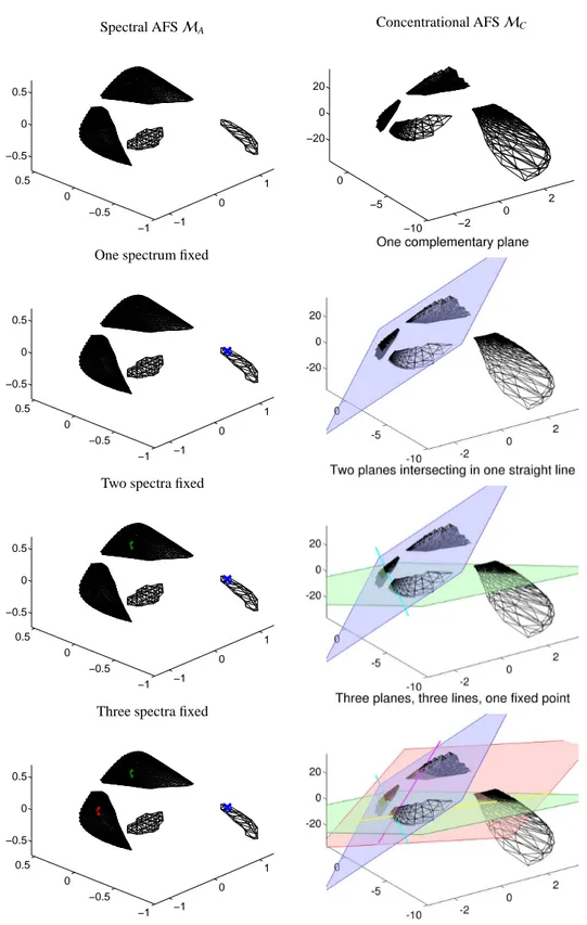
First the areas of feasible solutionsM_C andM_A for D are computed. Every AFS consists of four separated segments which can be associated with the four components of the model problem. These segments are each approximated by a polyhedron whose surface is a 3D triangle mesh. These triangle meshes are shown in the first row of images in Figure 6. Then a first spectrum A(1,:) is fixed and the representative x∈R³ is marked by a blue×inM_Atogether with a plane inM_Cto which C(:,2 : 4) are restricted; see the second row of images in Figure 6. If a second spectrum A(2,:) is given whose

representative is marked by a green ×in M_A, then a second plane can be added to M_C. The intersection of these two planes inM_C is a straight line (drawn by cyan color). This intersection combines the restriction on C(:,2 : 4) and C(:,[1,3 : 4]) so that the concentra- tion profiles C(:,3 : 4) are described, see third row in Figure 6. Clearly, C(:,1) is still represented by some point on the green plane and C(:,2) by some point on the blue plane. If a third spectrum A(3,:) is fixed, then a third plane is added toMAand C(:,4) is uniquely determined by the intersection of the three planes; see the last row in Figure 6. In the last image three lines are shown in cyan, yellow and magenta. These three lines are assigned to the three profiles C(:,i), i = 1,2,3, as pairs.

4.2.2. The simplices inMAandMC

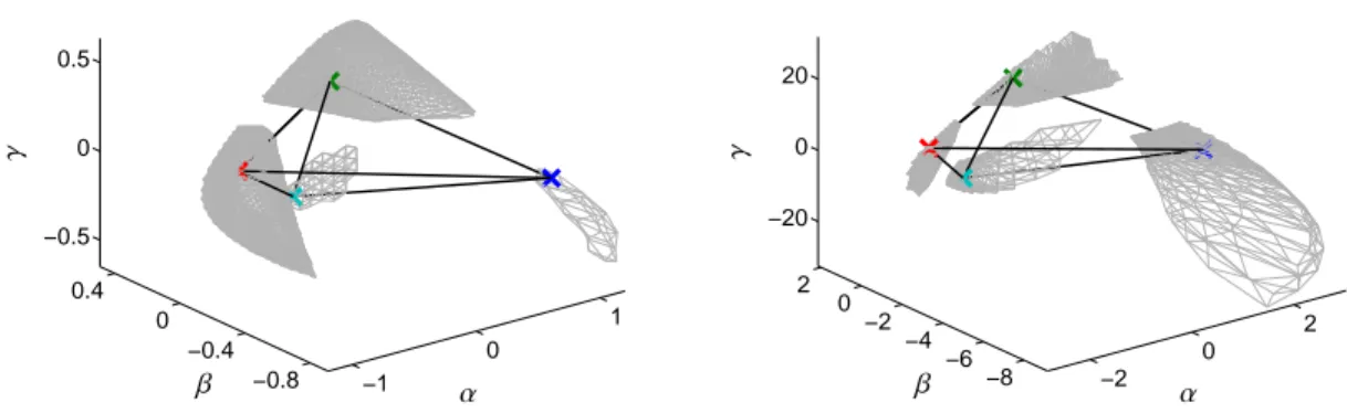
Theorem 3.5 describes the relation of the two simplices MA andMC which each uniquely determine a feasible factorization. For our four-component system such a pair of feasible simplices is shown in Figure 7.

These simplices are not independent of each other. As explained in Remark 3.6 the vertices of the simplices can be listed in the matrices T and Z and together with diagonal scaling matrices M1 and M2 a feasible nonnegative factorization can be written down in the form D=(UΣZ M2)(M1T V^T).

5. Conclusion

The AFS is a powerful tool to study the rotational ambiguity and the band of feasible solutions of multivariate curve resolution problems. However, the computation of all feasible solutions can only be a first step of a successful chemometric analysis of a spectroscopic data. Any further information on the reaction system should be used in order to decrease the rotational ambiguity. Such a decrease is equivalent with a reduction of the AFS. In the best case unique points in the AFS can be specified which uniquely determine one single factorization. A challenging point for the further application of AFS computations might be the analysis of multiway and multiset data [29]. Tauler, Maeder and de Juan [30] have devised a way how MCR-methods can be extended to the analysis of multiset data. Within this procedure the matricized form of the data can be an in- terface for the AFS techniques.

The complementarity theorem appears to be a valu- able tool in order to support this reduction process. Any feed-in of pre-given or suspected spectra or concentration profiles can be used in order to define certain affine 10

(11)

−1 0

1

−1

−0.5 0 0.5

Spectral AFSM_A

−2 0

2

−10

−5 0

−20 0 20

Concentrational AFSMC

−1 0

1

−1

−0.5 0 0.5

One spectrum fixed

−1 0

1

−1

−0.5 0 0.5

Two spectra fixed

−1 0

1

−1

−0.5 0 0.5

Three spectra fixed

Figure 6: Successive reduction of the rotational ambiguity for a four-component system. First row: AFSMAand AFSMC. Second row: A certain spectrum A(1,:) is fixed and Theorem 3.1 restricts C(:,2 : 4) to the blue plane. Third row: Two spectra A(1,:) and A(2,:) inM_A. The resulting two planes inM_Cintersect in a straight line (cyan) to which C(:,3 : 4) are restricted. The coupled concentration profiles C(:,1 : 2) in the sense of Theorem 4.6 in [20] are located on these planes. Fourth row: Three spectra are fixed, the coupled concentration profiles C(:,1 : 3) are each on one line (cyan, yellow, magenta) and the complementary concentration C(:,4) is uniquely given by the intersection of the three planes.

11

(12)

−1 0

1

−0.8

−0.4 0 0.4

−0.5 0 0.5

M_Aand the tetrahedron of solutions

β α

γ

−2 0

2

−6 −8

−2 −4 2 0

−20 0 20

MCand the tetrahedron of solutions

β α

γ

Figure 7: Tetrahedra or 3-simplices for the pure factors shown in Figure 5. The two tetrahedra are related according to Equation (12) in Theorem 3.5. The colors of the vertices are consistent with those of the pure factors in Figure 5.

spaces to which the remaining factor are restricted. If multiple information from different sources is used, then multiple affine subspaces can be formulated. The intersection of these subspaces in the AFS can easily be interpreted as a further strong reduction of the rotational ambiguity. The mathematical theory behind the reduction of the AFS by the complementarity theorem has been implemented to theFAC-PACKsoftware, see Section 3.3, and is available in its revision 1.1.

Acknowledgment

The authors would like to thank H. Abdollahi and members of his group for the inspiring discussions on the topic of this paper at the 4th Iranian Biennial Chemometrics Seminar in Shiraz, Iran, in November 2013.

6. Appendix

6.1. Complementarity theorem

Next the complementarity theorem is reproduced.

For its proof see [20].

Theorem 6.1. Let D ∈ R^k×n+ be a matrix of rank s, which is assumed to be decomposable in the form D= CA with nonnegative factors C ∈ R^k×s+ and A ∈ R^s×n+ . Let UΣV^Tbe a singular value decomposition of D. Fur- ther let the rows A(i,:) for i=1, . . . ,s0be given.

Then all the complementary concentration profiles C(:,j) for j=s₀+1, . . . ,s are contained in the (s−s₀)- dimensional linear subspace

{c∈R^k: c has the form c=UΣy for a vector y∈R^s which satisfies A(1 : s0,:)Vy=0}. (14)

The mathematical background of the complementarity theorem is the factorization

D=UΣV^T =UΣT⁻¹

| {z }

=:C

T V^T

|{z}

=:A

where T is an invertible s×s matrix. If some columns of C or some rows of A are known, then some linear constraints on T⁻¹ or on T can be derived. Then the identity T⁻¹T = I allows to translate these constraints to the inverse factor, i.e., on T or on T⁻¹. In a final step these relations can be formulated as conditions on the factor A or on the factor C. The linear space (14) is the result of this analysis.

References

[1] W.H. Lawton and E.A. Sylvestre. Self modelling curve resolu- tion. Technometrics, 13:617–633, 1971.

[2] O.S. Borgen and B.R. Kowalski. An extension of the multivari- ate component-resolution method to three components. Analyt- ica Chimica Acta, 174:1–26, 1985.

[3] R. Rajk´o and K. Istv´an. Analytical solution for determining feasible regions of self-modeling curve resolution (SMCR) method based on computational geometry. J. Chemometrics, 19(8):448–

463, 2005.

[4] M. Vosough, C. Mason, R. Tauler, M. Jalali-Heravi, and M. Maeder. On rotational ambiguity in model-free analyses of multivariate data. J. Chemometrics, 20(6-7):302–310, 2006.

[5] H. Abdollahi, M. Maeder, and R. Tauler. Calculation and Mean- ing of Feasible Band Boundaries in Multivariate Curve Res- olution of a Two-Component System. Analytical Chemistry, 81(6):2115–2122, 2009.

[6] H. Abdollahi and R. Tauler. Uniqueness and rotation ambigu- ities in Multivariate Curve Resolution methods. Chemometrics and Intelligent Laboratory Systems, 108(2):100–111, 2011.

[7] A. Golshan, H. Abdollahi, and M. Maeder. Resolution of Ro- tational Ambiguity for Three-Component Systems. Analytical Chemistry, 83(3):836–841, 2011.

12