A ray casting method for the computation of the area of feasible solutions for multicomponent systems: Theory, applications and FACPACK-implementation.

(1)

A ray casting method for the computation of the area of feasible solutions for multicomponent systems: Theory, applications and FACPACK-implementation.

Mathias Sawall^a, Klaus Neymeyr^a,b

aUniversit¨at Rostock, Institut f¨ur Mathematik, Ulmenstrasse 69, 18057 Rostock, Germany

bLeibniz-Institut f¨ur Katalyse, Albert-Einstein-Strasse 29a, 18059 Rostock

Abstract

Multivariate curve resolution methods suffer from the non-uniqueness of the solutions. The set of possible nonnegative solutions can be represented by the so-called Area of Feasible Solutions (AFS). The AFS for an s-component system is a bounded (s−1)-dimensional set. The numerical computation and the geometric construction of the AFS is well understood for two- and three-component systems but gets much more complicated for systems with four or even more components.

This work introduces a new and robust ray casting method for the computation of the AFS for general s-component systems. The algorithm shoots rays from the origin and records the intersections of these rays with the AFS. The ray casting method is computationally fast, stable with respect to noise and is able to detect the various possible shapes of the AFS sets. The easily implementable algorithm is tested for various three- and four-component data sets.

Key words: nonnegative matrix factorization, area of feasible solutions, band boundaries of feasible solutions, polygon inflation, FACPACK.

1. Introduction

In computer graphics ray tracing is the fundamental method for producing views of three-dimensional objects on a computer screen. A forerunner of ray tracing is the so-called ”ray casting” as presented by Appel in 1968 [3]. The basic idea of ray casting is to shoot light rays from the eye of an observer to his neighborhood and to detect the nearest blocking objects in the path of these rays. These points are used to cast the visi- ble surface of the objects. Here we extend the idea of ray casting in a way that we record the path of the ray through the object. By assembling all these in-object paths we approximate the shape of the complete object.

We use this algorithm in order to approximate the shape of certain bounded sets which represent the set of all possible nonnegative matrix factorizations (NMF) of a given spectral data matrix in chemometrics. Next we introduce the chemometric problem.

The series of spectra taken from a chemical reaction system can be stored in the rows of a matrix D. Mul- tivariate curve resolution (MCR) methods aim at ex- tracting from these superposed multicomponent spectral data the pure component information. If the chem- ical reaction system contains s chemical components,

then we are interested in matrix factorizations D=CA, where C contains in its s columns the concentration pro- files (along the time axis) of the pure components and where A contains in its s rows the associated pure com- ponent spectra. Thus D =CA is the matrix form of the Lambert-Beer law. The key difficulty of this matrix factorization problem is the so-called rotational ambiguity of the solution [44, 2]. This means that many factoriza- tions D =CA exist with nonnegative factors C and A.

For reaction systems with two components this ambiguity was first analyzed by Lawton and Sylvestre [21].

Later Borgen and Kowalski [7] as well as Rajk ´o and Istv´an [32] extended this analysis to three-component systems. These authors use the Area of Feasible Solu- tions (AFS) in order to represent the set of all nonnegative/feasible solutions in a low-dimensional way. Ef- fective numerical algorithms for the approximate computation of the AFS have been devised by Golshan, Ab- dollahi and Maeder [12] as well as Sawall, Neymeyr et al. [37, 38]. An alternative approach is the direct computation of minimal and maximal band boundaries as suggested by Gemperline [9] and Tauler [43]. See also [11] for a review on recent AFS methods.

A strong advantage of the AFS approach is that it makes available all NMFs. One might call this a global

October 6, 2016

(2)

approach. Hence the AFS comprises all the solutions which can be put out by any MCR method. It is a well- known fact that different MCR methods may result in very different results. Having computed the AFS for a given spectral data matrix, various post-processing techniques can help to eliminate chemically non-relevant solutions in the AFS. This reduction can be done in a controlled and steerable way. To this end, additional soft constraints can be used to reduce the AFS, see [4, 41, 31]. Alternatively, computational techniques like the window factor analysis [26], the evolving factor analysis [24, 22] or kinetic modeling [8, 33] can be em- ployed. See also Malinowski [25], Hamilton and Gem- perline [17] as well as Maeder and Neuhold [23] for a general and deepened introduction to MCR.

The aim of this paper is to present ray casting as a robust and fast numerical method for the computation of the AFS. In principle, ray casting can be applied to chemical reaction systems with any number of compo- nents. If the spectral data matrix D belongs to a chemi- cal reaction system which includes a number of s chem- ical components and D is a rank-s matrix, then the AFS is a bounded (s−1)-dimensional set. The ray casting al- gorithm records the paths of “equiangular” rays starting at the origin on its way through the AFS. All these paths serve to approximate the AFS.

In particular, we demonstrate applications to three- and four-component systems. For four-component systems the ray casting method has been implemented in a new module of the FACPACK software [39]. In a further new software module the complementarity and coupling theory [29, 36, 40, 34] has been implemented for four- component systems.

Organization of the paper: Section 2 briefly introduces the AFS concept and the fundamentals of its numerical approximation. In Section 3 important properties of the AFS are explained and the new gap-free intersection property is introduced and proved. The ray casting method is explained and discussed in Section 4.

Section 5 presents the background of its FACPACK im- plementation. Finally, numerical results for three- and four-component systems are presented in Section 6.

2. The AFS

2.1. Curve resolution methods

The basic equation for the two-way curve resolution problem is the Lambert-Beer law. Its matrix formula- tion in absence of noise reads

D=CA

with the spectral (mixture) data matrix D ∈ R^k×n and with C ∈ R^k×s and A ∈ R^s×n. The number k stands for the number of measured spectra and n is the num- ber of spectral channels of each spectrum. Further, s denotes the number of independent components with s ≤min(k,n). Our problem is to extract from given D the “true” chemically meaningful pure component de- composition D = CA. As already mentioned in the introduction, the rotational ambiguity makes this factorization problem hard to solve. It is an ill-posed problem.

The chemometric literature contains many techniques and algorithms to compute more or less suitable factorizations. Sometimes only parts of the factors are computed. All this reduces the rotational ambiguity. Among many others, some of these MCR approaches are hard- modeling techniques [16, 8], window factor analysis [24, 22, 26] in combination with uniqueness theorems [27], complementarity and coupling theorems [34] and soft modeling [44, 30, 13].

Instead of focusing on a single factorization, one can take up the challenge to compute the set of all NMFs of D. We call such factorizations with C ≥ 0, A ≥ 0 and D = CA feasible solutions. In the following, we describe techniques to get the set of all feasible spec- tral factors A≥0. A set of matrices is difficult to han- dle. However, the AFS provides an approach for a low- dimensional representation of these matrices. The key idea is to consider only the expansion coefficients of the possible spectra with respect to a basis of right singu- lar vectors of the matrix D. The AFS is introduced in Section 2.3; see also [7, 32, 12, 37, 38, 19, 35].

2.2. SVD-based factorization

The most usual way to solve the factorization prob- lem D = CA is to start with a singular value decom- position (SVD) of D ∈ R^k×n. The SVD has the form D =UΣV^T. For an s-component system and if D has the rank s, then s singular values are larger than zero.

These nonzero singular values are the diagonal elements of the diagonal matrixΣ∈R^s×s. The columns of the or- thogonal matrices U ∈ R^k×s and V ∈ R^n×sare the left and right singular vectors. The concentration profiles of the pure components are presented by a linear expansion in terms of the left singular vectors. The pure component spectra are presented by expansions in terms of the right singular vectors. These representations of C and A can be expressed by an invertible matrix T ∈ R^s×s (whose matrix elements are the expansion coefficients for A) so that

D=UΣV^T =UΣT| {z }⁻¹

C

T V^T

|{z}

A

, (1)

2

(3)

see [21]. The expansion coefficient of the first right singular vector and the left singular vector are always nonzero as otherwise A or C would have negative en- tries; see Theorem 2.2 in [38] for the mathematical jus- tification by the Perron-Frobenius theory on properties of eigenvalues and eigenvectors of nonnegative matrices. This together with a scaling argument justifies that the first column of T can be filled with ones, i.e.

T (i,1)=1, i=1, . . . ,s.

2.3. The AFS

A permutation can be applied to the rows of T in (1). The inverse permutation must be applied simultane- ously to the columns of T⁻¹. Thus the set of all possible nonnegative spectra is completely represented by the set of all possible first rows of T . This is the basic idea be- hind the AFS construction. Therefore the AFS consists of all row vectors x∈R^1×(s−1)so that

T =







1 x₁ · · · xs−1

1...

S

1







(2)

in (1) leads to feasible factors C=UΣT⁻¹≥0 and A= T V^T ≥0. Therein S is a proper (s−1)×(s−1) matrix which is to be determined, e.g., by an optimization. We denote the AFS byM. ThusMhas the form

M={x∈R^1×(s−1): T in (2) is a regular matrix, (3) C=UΣT⁻¹≥0 and A=T V^T ≥0}. (4) The analysis and geometric construction of the AFS was first studied for two-component systems in [21].

In [7, 32, 19] the AFS is geometrically constructed for s = 3 components. Numerical methods for the AFS-approximation for three-component systems are the brute-force grid search approach [2], the triangle- boundary-enclosure algorithm [12] and the polygon- inflation method [37, 38]. The paper [10] contains a recent application of polygon-inflation. For s = 4, up to now only the sliced triangle-boundary-enclosure algorithm has been introduced, see [14]. The algorithmic idea of polygon-inflation [37] can also be extended to a polyhedron inflation for four-component systems.

For the numerical approximation of the AFS the cru- cial step is to decide whether a certain point x is feasible or not. This step is also the computationally most time- consuming part of the algorithm due to its repeated application. For the feasibility decision we use the target

function f :R^(s−1)×R(s−1)×(s−1)→Rdefined as f (x,S )=

Xs i=1

Xk j=1

min(0,Cji)²

+ Xs

i=1

Xn j=1

min(0,Ai j)²+kIs−T T⁺k²_F. (5)

With this f the AFS has the form M={x∈R^1×(s−1): min

S∈R(s−1)×(s−1)f (x,S )=0}.

For data including noise, nonlinearities or perturbations the function f needs to be modified, see for example f from [37].

In the following we also need an important superset ofMwhich contains all x so that the linear combina- tions (1,x)·V^T are componentwise nonnegative

M⁺={x∈R^1×(s−1): (1,x)·V^T ≥0}. (6) The setM⁺is called FIRPOL by Borgen and Kowalski [7]. Geometrically FIRPOL is a polygon which speci- fies the outer boundary of the set of the feasible vectors x.

3. The gap-free intersection property of the AFS This section explains the three important properties which constitute the basis for the new ray casting method. These properties are:

1. Boundedness: The AFS is a bounded set.

2. Exclusion of the origin: The origin of the AFS for an s-component system, namely the point 0 ∈ R^s−1, is never an element of the AFS M. How- ever, 0 is always contained inM⁺(FIRPOL), see Eq. (6).

3. Gap-free ray intersection: The intersection of the AFS with a ray starting at the origin is empty or a line segment. The line segment may be degenerated to a single point. In other words, this intersec- tion is gap-free.

The first two properties are not new and are recapitu- lated in Section 3.1. The new ray intersection property is proved in Section 3.2 by Theorem 3.3.

3.1. Boundedness of the AFS and position of the origin The boundedness of the AFS is a necessary prereq- uisite for all numerical algorithms to compute the AFS.

Theorem 2.3 in [38] shows that the AFS is bounded if and only if the matrix D^TD is irreducible. This is a mild 3

(4)

condition which can be assumed to hold whenever the spectral data, loosely speaking, does not allow to split the data matrices into independent reaction subsystems.

The second property claims that the origin is an element ofM⁺(FIRPOL), but is never an element ofM (AFS). Since the first right singular vector3₁can be assumed as a componentwise nonnegative vector by the Perron-Frobenius theory, see Lemma 3.1, it holds that

(1,0, . . . ,0

| {z }

s−1-times

)V^T =3₁≥0.

Thus x=0 is an element ofM⁺according to Equation (6). Further, Theorem 2.5 in [38] proves that the origin is not an element ofM.

3.2. The gap-free intersection property

This section presents and proves the ray intersection property of the AFS, which is the basis for the ray casting method. The idea can easily be explained: If a ray is shot from the origin and if the ray hits the surface of the AFS at a certain point x of the AFSM, then the intersection of this ray with the AFS consists of all points γx with 1 ≤ γ ≤γ^∗so thatγ^∗x belongs to the surface of the set FIRPOLM⁺, see Figure 1. In other words a nonempty intersection of such a ray with the AFS is a line segment (which may degenerate to a single point).

This intersection property is proved by Theorem 3.3.

First, two preparatory lemmata are needed.

Lemma 3.1. Let D ∈ R^k×n be a nonzero nonnegative matrix. Let UΣV^T be a singular value decomposition of D. If the first singular vector V(:,1) is a component- wise nonnegative vector, then the first left singular vec- tor U(:,1) is also a componentwise nonnegative vector.

(The Perron-Frobenius theory [28] guarantees that non- negativity of V(:,1) can always be attained by a proper choice of this singular vector.)

Proof. The equation DV=UΣimplies that DV(:,1)=U(:,1)σ1

withσ1 >0 since D,0. Thus V(:,1)≥0 and D≥0 show that DV(:,1)≥0. Hence U(:,1)≥0.

Lemma 3.2. Let C∈R^k×sand A∈R^s×nbe nonnegative matrices. Further let

X= β b^T

0 I

!

∈R^s×s (7)

withβ ≥ 1 and b ∈ R^s−1 with b ≤ 0 componentwise.

Further, I denotes the (s−1)×(s−1) identity matrix.

Then

e

C=CX⁻¹ (8)

is a nonnegative matrix. Moreover X(1,:)A≥0 implies that

e

A=XA (9)

is also a nonnegative matrix.

Proof. Direct computation shows that X⁻¹= 1/β −b^T/β

0 I

! .

The assumptions on βand b imply that X⁻¹ is a nonnegative matrix. ThusCe= CX⁻¹ is also nonnegative.

By assumption A(1,e :) = X(1,:)A is nonnegative. For the remaining rows ofA the equations (7) and (9) implye that

e

A( j,:)=A( j,:)≥0 for j=2, . . . ,s.

This provesAe≥0.

Lemmata 3.1 and 3.2 together with Corollary 2.3 from [38] help to prove that nonempty intersections of the AFS with rays starting at the origin are line segments. A line segment may even be degenerated to a single point.

Theorem 3.3 (On the intersections of rays with the AFS). Let D ∈ R^k×n be a nonnegative matrix with no zero-column, no zero-row and rank(D)=s so that D^TD and DD^Tare irreducible matrices. Let UΣV^Tbe a trun- cated SVD of D with V(:,1)>0.

If x∈ M, then a numberγ^∗≥1 exists so thatγ^∗x is located on the boundary ofM⁺(FIRPOL) and the line segment

{γx : γ∈[1, γ^∗]} is a subset of the AFSM.

Proof. The feasible point x∈ Mbelongs to a matrix T of the form (with the all-ones vector e = (1, . . . ,1)^T ∈ R^s−1)

T = 1 x^T

e S

! 4

(5)

so that C=UΣT⁻¹and A=T V^Tare nonnegative matrices. Our aim is to show thatCe=UΣeT⁻¹ andAe=T Ve ^T are also nonnegative with

e

T = 1 γx^T

e S

!

for anyγ∈[1, γ^∗]. Thus with X=T Te ⁻¹we have e

C=(UΣT⁻¹)

| {z }

C

(TTe⁻¹)

| {z }

X⁻¹

and Ae=(eT T⁻¹)

| {z }

X

(T V^T)

|{z}

A

which is a representation ofC ande A according to (8)e and (9). In the following we show that X satisfies the assumptions of Lemma 3.2. Then Lemma 3.2 proves the desired nonnegativity ofC ande A. The inverse of thee 2×2 block matrix T reads

T⁻¹= 1+x^TZ⁻¹e −x^TZ⁻¹

−Z⁻¹e Z⁻¹

!

(10) with the Schur complementZ = S −ex^T, see [15].

(One can easily check that T T⁻¹ = I holds.) Lemma 2.3 in [38] says that a componentwise nonnegative vec- tor UΣw necessarily requires that the first component w₁ is nonzero. Under our assumptions on D and the SVD, Lemma 3.1 says that U(:,1)≥ 0. Hence w1 >0 must hold as otherwise for w1<0 the vector UΣw necessarily contains negative components. This argumentation ap- plied to each column of C=UΣT⁻¹implies that the first row of T⁻¹by (10) is strictly positive. In other words we have that

x^TZ⁻¹<0 (11)

holds. The sum of the components of x^TZ⁻¹ equals x^TZ⁻¹e. We conclude from (11) that

x^TZ⁻¹e<0. (12) The two inequalities (11) and (12) are used in the final part of the proof.

The Sherman-Morrison formula [15] allows to write the inverse Schur complement explicitly

Z⁻¹=S⁻¹+S⁻¹ex^TS⁻¹ 1−x^TS⁻¹e. Direct computation shows that

X= 1−(γ−1)x^TZ⁻¹e (γ−1)x^TZ⁻¹

0 I

! .

Asγ≥1, we see that the vector b in (7) equals b=(γ−1)x^TZ⁻¹

and that b ≤ 0 componentwise due to (11). Thus the first assumption of Lemma 3.2 is fulfilled. Further,β= 1−(γ−1)x^TZ⁻¹e≥1 since x^TZ⁻¹e<0 by Eq. (12) andγ≥1. Thus the second assumption of Lemma 3.2 is fulfilled. So Lemma 3.2 guarantees thatCe=CX⁻¹is a componentwise nonnegative matrix.

Finally, we have to show that Ae = XA is a com- ponentwise nonnegative matrix. Lemma 3.2 says that X(1,:)A≥ 0 is sufficient for the nonnegativity ofA. Ite holds that

X(1,:)A=a^T₁ −(γ−1)h

x^TZ⁻¹ea^T₁ −x^TZ⁻¹A([2 : s],:)i

| {z }

=:r

where a^T₁ denotes the first row of A. Forγ=1 the spec- trum a^T₁ is feasible by assumption, i.e. a^T₁ ≥0. Further, forγ=γ∗

X(1,:)A=a^T₁ −(γ^∗−1)r

is also feasible by assumption so that a^T₁−(γ^∗−1)r≥0.

Finally, γ^∗ > 1 can be assumed. Multiplication of the last inequality by the nonnegative constant (γ−1)/(γ^∗− 1) withγ≥1 results in

(γ−1)/(γ^∗−1)a^T₁−(γ−1)r≥0.

Asω :=1−((γ−1)/(γ^∗−1))≥0 for 1≤γ≤γ^∗we can addωa^T₁ ≥0 to the last inequality which results in

a^T₁ −(γ−1)r≥0

which shows that X(1,:)A≥0. Lemma 3.2 provesAe≥ 0.

Theorem 3.3 implies Corollary 3.4.

Corollary 3.4. On the assumptions of Theorem 3.3 let x be a point on the boundary ofM⁺(FIRPOL). If x is not feasible, then the ray which starts at the origin and which runs through x contains no feasible point.

Proof. Assume the existence of a point y = ωx ∈ M with 0 < ω < 1. Then Theorem 3.3 says that the line segment from y to x is contained in the AFS. This con- tradicts the assumption that x is not in the AFS.

4. The ray casting method

This section provides a detailed explanation of the new ray casting algorithm for approximating the AFS.

The single steps of the algorithm are fundamentally based on the three properties of the AFS, namely the 5

(6)

−0.5 0 0.5 1 1.5

−0.5 0 0.5

Outer bounds and rays

−0.5 0 0.5 1 1.5

−0.5 0 0.5

Feasible end-points on the rays

−0.5 0 0.5 1 1.5

−0.5 0 0.5

Enclosure of the AFS

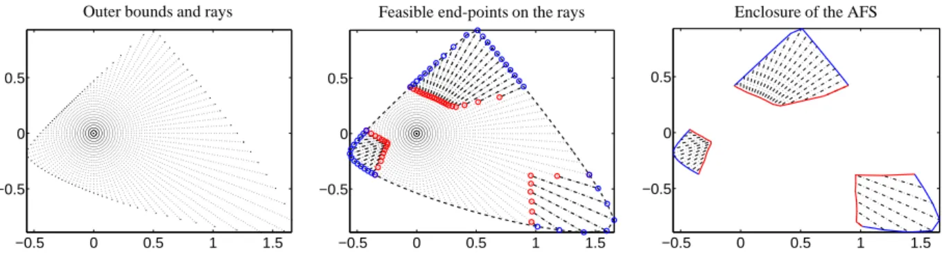
Figure 1: Construction of the 2D AFS for a three-component system by m=100 rays. Left: Equiangular ray casting with ray directions3_i ∈R² (step 1). Computation of outer bounds radii Ri(step 2). Center: Computation of the inner radii ri(step 3). The points of the setR^outare marked by blue circles and the points of the setRⁱⁿare marked by red circles. Right: Connection of the inner and outer points (step 4). The boundary sections on the boundary of FIRPOL are colored in blue. Boundary sections on the inner boundary are colored in red. Also, the connecting lines between inner and outer boundaries are colored in red. For demonstration purposes the angle-resolution is very low. Typically much more than m=100 rays are used.

boundedness, the exclusion of the origin and the gap- free ray intersection, see Section 3. The ray casting al- gorithm works with equiangular rays (e.g. in polar coordinates) which start at the origin. The origin is never a feasible point. If a certain point x is feasible, then the complete line segment of this ray from x to the bound- ary ofM⁺(FIRPOL) belongs to the AFS. Conversely, if the intersection of the ray with the boundary ofM⁺ is not a feasible point, then the intersection of this ray with the AFS is empty. Computationally, we first check the feasibility of this point of intersection. In a second step, we look for the point on this ray which is feasible and closest to the origin. In a final step, all these extremal points are connected in order to approximate the boundary of the AFS.

4.1. Notation and algorithm

We consider a number of m vectors3_i, i=1, . . . ,m, starting at the origin of the AFS. An exemplary, equiangular 2D setting of these vectors is shown in Figure 1 (left subplot) and a 3D setting is shown in Figure 2 (left subplot). For ease of presentation we do not distinguish the vectors3_i from the rays{c3_i : c ≥ 0}. If the ray 3_i hits the AFS, then two radii are determined. These are the minimal radius r_i, i.e. the distance of the closest AFS-point on3_i to the origin, and the maximal radius R_i, which is the maximal distance of an AFS-point on this ray to the origin. Mathematically, these radii for a given ray3_iare

ri=min

γ >0 with min

S f (γ3_i,S )=0

, (13)

Ri=max

γ >0 with min

S f (γ3_i,S )=0

(14)

with f (x,S ) by (5). Hence Riis the distance of the point of intersection of the ray 3_i with the boundary ofM⁺ (FIRPOL). Theorem 3.3 proves that the line segment

{γ3_i: ri≤γ≤Ri} (15) equals the intersection of the ray 3_iwith the AFS. We denote byRⁱⁿthe set of all points with minimal radii on the rays3_i, i =1, . . . ,m, and byR^outthe corresponding set of points with maximal radii.

The steps of the ray casting algorithm are as follows:

1. Assign a number of m equiangular rays3_iin the (s−

1)-dimensional space, e.g., by using (generalized) polar coordinates.

2. For each ray compute the maximal radius R_iso that Ri3_iis located on the surface ofM⁺(FIRPOL).

3. For each ray test whether Ri3_i∈ Mor not. If Ri3_i∈ M, then compute the minimal radius r_i=min{γ >

0 : γ3_i∈ M}.

4. Connect the matching interior points ri3_iand asso- ciated exterior points Ri3_iin order to approximate the boundary of (a segment) of the AFS.

4.2. Computation of the extremal points

For noise-free data the computation of the maximal radius Rican either be done by direct evaluation of the nonnegativity constraints or alternatively by means of numerical bisection. The computational costs are low as only the FIRPOL constraint (1,x)V^T ≥ 0 is to be checked along the ray. The computation of the radius riis done by using the bisection method along each ray.

We use the bisection method with an additional control parameterεbin a way that

min

S f (ri3_i,S )=0 and min

S f ((ri−εb)3_i,S )>0 (16) 6

(7)

−1 0

1 −1 −0.50 0.5

−0.5 0 0.5

x₁

x2

x3

outer bounds and rays

−1 0 1 −1 −0.50 0.5

−0.5 0 0.5

x₁

x2

x3

feasible points on the rays

−2 0

2 −1 0

1

−0.5 0 0.5

x1

x2

x3

enclosed AFS

Figure 2: Computation of a three-dimensional AFS for a four-component system (s=4) with m=512 rays. Left: 512 rays3_i ∈R³(step 1) are shown with end-points on the boundary of FIRPOL. The length of the ray3_iis Ri(step 2). Center: Computation of the inner radii ri(step 3). Only feasible directions are plotted. Right: Matching points on the surfaces of the segments of the AFS are connected by grid lines (step 4). As in Figure 1 the points and lines on the outer boundary are drawn in blue and those on the inner boundary are drawn in red.

with f by (5). In each step a nonlinear optimization problem on finding a proper S must be solved. Thus the computational costs are relatively high.

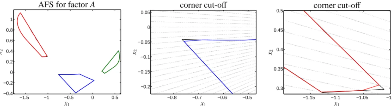
4.3. Precision, resolution and corner cut-off

The numerical accuracy of the radii r_iand R_ican be controlled by the parameterεbin (16). The density of the extremal pointsRⁱⁿ andR^out on the surface of the AFS is determined by the number of rays m. A large number m of rays results in a fine lateral resolution of the boundary of the AFS.

A critical aspect of the ray casting method is that a low angle-resolution, i.e. m is small, may result in a corner cut-off. Especially if a first ray has a relatively large intersection with the AFS and a second adjacent ray contains no feasible point, then some part of the boundary of the AFS approximation is determined by the first ray. The cone between these two rays may in- clude a part of the AFS which is then cut off. An in- creased resolution by a larger number m of rays can reduce such a cut-offof boundary-near regions of the AFS. Figure 3 demonstrates a minor corner cut-offfor a two-dimensional AFS.

4.4. Two- and three-component systems

The computation of the AFS for two- and three- component systems (s=2 or s=3) is well-understood, see for example [21, 7, 32, 1, 2, 12, 37, 38].

For two-component systems (s=2) the AFS consists of two separated intervals, i.e.

M=[−R1,−r1]∪[r2,R2]

with the sets of positive minimal and maximal radiiRⁱⁿ andR^out, see Section 4.1,

Rⁱⁿ={r₁,r2}, R^out={R₁,R2}.

Computationally, these radii, which represent the boundaries ofM, can be determined by starting the al- gorithm with (the only possible) m = 2 rays given by 3₁=−1 and3₂=1.

For three-component systems (s = 2) the AFS is a subset of the planeR². A number of m equiangular rays is constructed in polar coordinates

3_i= cosφ_i sinφi

!

with φi=2πi−1

m , i=1, . . . ,m.

(17) Figure 1 shows the application to the model problem of a three-component consecutive reaction with shifted Gauss profile spectra taken from Section 2.1 of [39]. A number of m=100 rays are used for the approximation of the boundary of the AFS which consists of three isolated subsets, which we call the segments of the AFS.

4.5. Four components

For four-component systems (s = 4) the AFS is a three-dimensional set. Spherical coordinates can be used to construct evenly distributed (and with respect toφi,1andφj,2equiangular) rays

3_i+j=





sin(φi,1) cos(φj,2) sin(φi,1) sin(φj,2)

cos(φi,1)



, φi,1=πi−1

ℓ1

, φj,2=2πj−1 ℓ2

,

(18) for i=1, . . . , ℓ1and j=1, . . . , ℓ2. This allows to form m = ℓ1ℓ2 rays. Figure 2 shows the application to a model problem (D ∈ R^10×11 with C formed by Gaus- sians and A formed by partially overlapping and shifted Gaussians) withℓ₁=13 andℓ₂=32. However, the res- olution with m =512 rays is relatively low and is only used for demonstration purposes.

7

(8)

−1.5 −1 −0.5 0 0.5

−0.4

−0.2 0 0.2 0.4 0.6 0.8 1

x₁ x2

AFS for factor A

−0.8 −0.7 −0.6 −0.5

−0.2

−0.15

−0.1

−0.05 0 0.05

x₁ x2

corner cut-off

−1.15 −1.1 −1.05 −1

0.3 0.35 0.4 0.45 0.5

x₁ x2

corner cut-off

Figure 3: AFS approximations for the model problem from Sec. 6.1. Left: The colored boundary curves of the AFS have been computed by ray casting with m=300 rays with a boundary precision ofεb =10⁻³. The (for the most part underlying) black solid lines result from the polygon inflation method by the FACPACK software [38]. Center and right: Enlargements of the left-upper area of the blue AFS segment and the right lower area of the red segment. The dotted lines are the rays of the ray casting algorithm. A minor corner cut-offcan be stated, see Sec. 4.3.

4.6. Higher number of components

For s-component systems with s ≥ 5 the rays3_i ∈ R^s−1 can be constructed by using (s−1)-dimensional spherical coordinates [6]

3_i,1=cos(φi,1), 3_i,2=sin(φ_i,1) cos(φ_i,2), 3_i,3=sin(φi,1) sin(φi,2) cos(φi,3),

...

3_i,s−2=sin(φi,1)·. . .·sin(φi,s−3) cos(φi,s−2), 3_i,s−1=sin(φi,1)·. . .·sin(φi,s−3) sin(φi,s−2).

(19)

The discretization for the last angleφi,s−2is φi,s−2=2πi−1

ℓs−2

, i=1, . . . , ℓs−2, and for the remaining angles we use

φj=πi−1 ℓj

, i=1, . . . , ℓj, j=1, . . . ,s−3.

This general definition already includes the cases of polar coordinates (s=3) and 3D spherical coordinates (s=4). The total number of rays is m=ℓ1ℓ2. . . ℓs−2. 4.7. Stability for the various shapes of an AFS

In general, the AFS can be a topologically connected set with holes, or the AFS can consist of several isolated subsets, the segments of an AFS. Especially for two-component systems the AFS consists of two separated intervals, one only in the negative numbers and the other only in the positive numbers. For s =3 the AFS is well known to be either a single-segment AFS with a hole around the origin [37, 38] or it consists of three

isolated segments. Additionally, nonnegative matrices can be constructed whose AFS consists of 6 segments, 9 segments or even higher multiples of 3 segments. How- ever, an AFS for a real chemical reaction system with more than 3 segments is not known up to now. For s=4 there is no general presumption on the possible number of segments. Figure 7 shows an AFS with four clearly separated segments. Further Figure 9 presents a single- segment AFS with a complicated ”Swiss-cheese like”

hole structure. Further experiments have shown that the AFS for the case s=4 may also have a closed surface with no holes going through to the origin. However, the origin is never contained in the AFS - any AFS has a hole around the origin.

The ray casting algorithm is general and flexible enough to compute approximations of all AFS types.

The gap-free intersection property of the AFS by Theo- rem 3.3 guarantees that the ray casting algorithm can work successfully for any number s of components.

This is a main advantage compared to the triangle- boundary-enclosure algorithm [12, 14] or the basic polygon inflation method [37]. However, the inverse polygon inflation algorithm [38] and the geometric constructive Borgen plot approach [7, 32, 19] also work for any AFS of a three-component system.

4.8. Factor-locking

Sometimes certain pure component spectra or concentration profiles are known, e.g., a spectrum of the main reactant or main product. This additional information reduces the rotational ambiguity [34, 29]. If par- ticular columns of C or rows of A are available, then the equation D=CA provides some information on the other factor (A or C). See, for example, [5, 40, 29] for a systematic analysis of these mutual restrictions for sys- tems with s=3 or s=4 chemical components. Given 8

(9)

.

3₁

3₂ 3

3

3₄

w

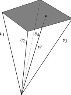
Figure 4: Detection of degenerated AFS segments: The initial ray w (computed by an NMF) has a feasible point on the surface ofM⁺(FIRPOL).

The gray rectangle is a part of the surface ofM⁺. The pyramid spanned by the closest neighboring rays3_i, i=1, . . . ,4, serves to check the degree of degeneracy of the AFS segment whether it is a line segment or plane segment.

components are represented in the AFS by fixed points.

This type of additional information is called an equality constraint [5]; in the FACPACK software [38] equality constraints can be set by factor-locking. Such a constraint also reduces the size of the AFS segments for the remaining unknown factors.

Remark 4.1. Let one or more points in the AFS be given, i.e. certain pure component spectra or concen- tration profiles are fixed. Then the gap-free intersection property (see Theorem 3.3) still holds for the reduced AFS-segments of the remaining components.

The proof of Remark 4.1 is very similar to the proof of Theorem 3.3. Once again, one can prove that the sub- matrix S of T which represents a certain vector x of the AFS can also be used to represent the stretched point γx. Locked points of the AFS are represented by cer- tain components of S which remain unchanged. Hence, γx is feasible also in the presence of these locked points.

Essentially, Remark 4.1 says that the ray casting algorithm can be applied without changes to the case of ac- tive equality constraints. The resulting AFS is a subset of the original AFS (only under nonnegativity constraints).

5. Software implementation in FACPACK

The FACPACK-toolbox is a collection of several SMCR methods with the focus on global AFS methods [39]. The software contains implementations of the polygon inflation method and its variants [37, 38], of the geometric-constructive Borgen-plots [7, 32, 19], of the complementarity theorem [40] and its restrictions on the AFS [40] and so on. FACPACK is equipped with a graphical user interface in MatLab. The computational cores of the program are written in C. The toolbox can be downloaded from

http://www.math.uni-rostock.de/facpack/

The latest revision of the software includes a module for computing the three-dimensional AFS for (s = 4)- component systems by means of ray casting. Addition- ally, a further new module implements the complementarity theory [34] for four-component systems by means of ray casting.

5.1. Refinement process

The minimal and maximal radii r_i and R_i, see Eqns. (13) and (14), are computed for each ray by solv- ing nonlinear optimization problems. The numerical results of these optimizations, especially for the inner points, depend on good initial guesses. In order to iden- tify and to rule out wrongly classified points, a refinement post-process is started at the end of the AFS com- putation. The reliability of each minimal radius ri is checked by restarting the optimization process with various initial values. These initial values are taken from the already computed inner radii of the closest neighboring rays.

5.2. Approximation of degenerated AFS segments A special challenge for any numerical approximation of the AFS are cases in which the s-dimensional AFS contains lower dimensional segments.

An important example is a three-dimensional AFS for a four-component system which contains planar, linear or punctiform segments. The new 3D-AFS module of FACPACK can compute all these types of AFS seg- ments. Therefore the algorithm does not only compute the minimal and maximal radii for the m rays, but also uses the initial NMF of the spectral data matrix D. For a four-component system, the initial NMF provides four feasible points and these define the directions of four 9

(10)

initial rays. If along one such ray the minimal radius and the maximal radius coincide, then this indicates a degenerated AFS segment. In such a case the algorithm checks the four closest neighboring rays; see Figure 4 for an illustration of the pyramid spanned by the neighboring rays together with the enclosed initial ray from the NMF. If the minimal radius and the maximal radius coincide for the initial NMF ray and if for all four neighboring rays the intersections with the AFS are either empty or consist of only a single point, then the AFS segment is degenerated. The algorithm has to distinguish planar segments from linear segments and from punctiform segments:

Planar segments:

If a certain AFS segment is not a volume segment, then the algorithm tests this segment for planarity. Any planar segment must be a subset of a plane which has been used for the construction of the surface of the poly- hedronM⁺ (FIRPOL). If an initial ray contains only one feasible point (necessarily this point is located on the surface ofM⁺), then an adapted polygon inflation method [37] is used in order to compute the boundary of the associated planar AFS segment, which is again located on the surface ofM⁺.

Linear segments:

If a segment is neither a volume segment nor a planar segment, then the algorithm tests this segment for linearity. In order to detect a line segment, we follow the optimization strategy on the search direction as described in Sec. 4.6 of [38]. In contrast to [38] we need two different angle variables in the optimization for the computation of a linear segment in 3D. Starting from a feasible point x∈R³(which might be gained by an initial NMF) the two anglesφ1andφ2are determined in a way so that the point

x+r





sinφ1cosφ2

sinφ1sinφ2

cosφ1



 (20)

is feasible for a sufficiently small nonzero radius r. Next the minimal and maximal bounds rl ≤0 and rr ≥0 on this line segment are computed so that the points on the line segment with rl ≤r ≤rrin (20) are feasible. The result is a feasible line segment.

Punctiform segments:

If the segment is not a volume segment, a planar segment or a linear segment, then it must be an isolated point. A unique pure component has been found.

Figure 5 shows the AFS for the upper triangular ma-

trix

D=







1 2 3 4

0 1 2 3

0 0 1 2

0 0 0 1





 .

Its AFS consists of a unique point, a linear segment, a planar segment and a volume segment. This simple rank-4 matrix comprises all difficulties of an AFS computation for segments with different dimensionalities in an elegant and easy way. ¹ This artificial example can principally be extended to a data matrix which corre- sponds to a chemically interpretable data set.

The unique point is computationally accessible from any initial NMF of D. The computation of the linear segment by means of a two-angle approach is described above. A first approximation of the planar segments di- rectly results from the ray casting algorithm. This approximation can be refined by applying the idea of the polygon inflation method within this plane. Then only two of the three coordinates x1, x2 and x3 are free variables. This procedure is similar to the slicing method from [14]; however the computed plane is usually not orthogonal to one of the coordinate axes.

5.3. Ray casting combined with soft constraints As demonstrated in [5, 4, 41, 31] and in further publi- cations, the AFS can significantly be reduced by applying soft constraints. A straightforward implementation of soft constraints like unimodality, closure or mono- tonicity may be inconsistent with the gap-free intersection property which is of central relevance for the ray casting algorithm. Equality constraints can easily be implemented, see Section 4.8 and Remark 4.1.

The key problem with the unimodality and mono- tonicity constraints is that it is not evident that Theorem 3.3 still holds for the constraint-restricted set M. At least, the property thatγ^∗x is located on the boundary of M⁺, see Thm. 3.3, has to be adapted in an appropriate way if additional constraints are used. A thorough analysis of these questions should be a topic of future work - the current work is devoted to the basic nonnegativity constraint.

6. Numerical results

Next the ray casting algorithm is applied to model problems with s = 3 and s = 4 components. The re- sults for s=3 are compared with the results gained by

1We are very grateful to Annekathrin J ¨urß, University of Rostock, for providing the idea behind this model problem.

10

(11)

0 2

−1 0 1 2 3 4 5 6 4

−4

−3

−2

−1 0 1 2

x₁ x2

x3

AFS with a unique point, a line-, a plane- and a volume-segment

Figure 5: The AFS for the upper triangular rank-4 matrix D∈R^4×4with Di j=max( j−i+1,0) consists of a unique point (cyan), a linear segment (red), a planar segment (green) and a volume segment (blue).

the polygon inflation method [37, 38] in its FACPACK implementation [39].

6.1. Three components

We re-use the model problem of a consecutive irre- versible reaction with three components from Sec. 4 of [37]; the unimodal model spectra are strongly overlap- ping. We use the associated data matrix D∈R^k×nwith k = 1000 and n = 1500. The AFS consists of three clearly separated segments. The ray casting algorithm is applied with m=300 rays. The bisection method uses the boundary precisionεb = 10⁻³, see Eqn. (16). The results are shown in Figure 3 together with the results of the polygon inflation method (by black lines which are for the most part covered by the colored lines).

The computation time of the ray casting algorithm is 66.9 seconds. The ray casting algorithm is written in C and the program code uses one core of a 2.4GHz Intel CPU on a standard PC with 16 GB RAM. For this two- dimensional AFS the adaptive polygon inflation method needs only 12 seconds; see also Table 2 in [37].

Next the precision of the results by ray casting is compared to the precision of the polygon inflation method. In order to measure the distance of the two AFS approximations we use the Hausdorffdistanceδ(A,B), which is the mutual deviation of two sets A and B

δ(A,B)=max

maxa∈A d(a,B),max

b∈B d(A,b)

. (21)

Therein d(a,B) = minb∈Bka−bk2 is the minimal dis- tance of a point a to a set B. We have computed the three

Hausdorffdistances separately for each of the three segments of the AFS. The results are

(δ₁, δ₂, δ₃)=(9.17·10⁻³, 5.00·10⁻³, 1.48·10⁻²).

For δ1 (blue segment in Figure 3) and δ2 (green segment) the distances are consistent with the boundary precision εb = 10⁻³. Forδ3 (red segment in Figure 3) the larger distance can be explained by the efficient spatial adaptivity of the polygon inflation method. In contrast to this, ray casting works with a fixed angular resolution, which can result in a certain corner cut-off, cf. Section 4.3.

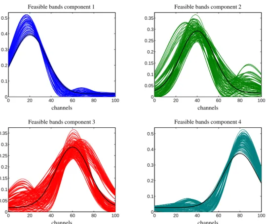
6.2. Four components with four isolated segments Next a model problem with s=4 components, k=70 spectra and n=50 channels is discussed. The factors C and A are shown in the left and centered plot of Figure 6. Ray casting uses m =5000 rays. The computation takes 447.4 seconds. The AFS consists of four isolated segments. Two segments are small and their distance to the origin is larger compared to the two remaining segments. Hence fewer rays hit these smaller segments.

For a proper approximation of these two segments we have increased the ray density by the factor 4. The resulting AFS is plotted in Figure 7. The associated series of spectra, the so-called feasible bands, are plotted in Figure 8.

6.3. Four components with a single-segment AFS By adding constant offsets to the four spectra from Section 6.2, the overlap of these spectra is increased.

11

(12)

0 20 40 60 80 100 0.2

0.4 0.6 0.8 1

time

Conc. profiles (for Sec. 6.2 and 6.3)

0 20 40 60 80 100

0 0.2 0.4 0.6 0.8 1

channels Pure comp. spectra (Sec. 6.2)

0 20 40 60 80 100

0 0.2 0.4 0.6 0.8 1 1.2

channels

Spectra with offset (data section 6.3)

Figure 6: The pure components of the two model problems discussed in Section 6.2 and 6.3. Left: The same concentrational factor C is used for the two model problems. Center: Spectral factor A for the model problem from Section 6.2. The resulting AFS is shown in Figure 7. Right: Spectral factor which underlies Section 6.3 with added offsets which increase the overlap between the spectra. The resulting single-segment AFS is shown in Figure 9.

The factor C remains unchanged; see left subplot in Fig- ure 6. The resulting AFS of D=CA is plotted in Figure 9. The AFS is a topologically connected set with three holes. Compared to the first 3D AFS much more rays hit the AFS. Hence the computation time increases to 1889 seconds.

7. Application to FT-IR experimental data

Next the ray-casting method is applied to experimental and noisy in-situ FT-IR data of a three-component system. The results are compared with those gained by the polygon inflation method.

7.1. Hydroformylation data

The in-situ FT-IR data have been taken from the hydroformylation of 3,3-dimethyl-1-butene with a phosphite-modified rhodium catalyst, see [20]. Here we consider only the spectral window [1963,2116]cm⁻¹ since this interval contains the characteristic signals from three components, namely the olefin, if the acyl complex and the hydrido complex, see [20]. The wavenumber grid has n=639 channels. With k =850 spectra the matrix D has the dimensions 850×639.

7.2. AFS computations

For this three-component system we compute the AFS for the spectral factor A by means of the ray casting algorithm. The results are compared to those of the polygon inflation algorithm. The ray casting method is run six times with m ∈ {100,200,300,400,500,1000,5000}. The boundary precision is ε = 10⁻³ for all computations and four sweeps of refinement have been applied. The FACPACK-implementation of the polygon inflation method is used with the default control parametersεb=

δ=10⁻³, see [37, 38] for details on the control parameters.

For these computations ray casting and polygon inflation use the same control parameter ε = 0.005 as a lower bound for the acceptable relative nonnegativeness of the factors in the sense

j=1,...,kminC( j,i) max

j=1,...,kC( j,i) ≥ −ε,

j=1,...,nmin A(i,j) max

j=1,...,nA(i,j) ≥ −ε, (22) for i=1, . . . ,s.

Figure 10 shows the results of ray casting with m = 1000 rays together with the results of polygon inflation.

The AFS consists of three isolated segments. The results are almost the same. The Hausdorffdistance measure by Eq. (21), which describes the distance between two sets, is applied to the corresponding pairs of AFS segments. The computation times for ray casting for different numbers of rays are listed in Table 1. The polygon inflation method needs only 6.45s. All computations have been run on a standard PC with a 2.4GHz Intel CPU (only one core is used) and 16 GB RAM.

The computation times increase linearly in the number of rays. The Hausdorff distances are consistent with the control parameters on the boundary precision εb=10⁻³.

These results support that the new ray casting algorithm is a proper tool for AFS computations. How- ever, for two- and three-component systems there are faster methods (e.g. polygon inflation and Borgen plots [7, 32, 19]). The true benefit of ray casting is its easy applicability to systems with four or even more components.

12

(13)

−1

−0.5 0

0.5 1

−0.6 −0.8

−0.2 −0.4 0.2 0

0.4

−0.6

−0.4

−0.2 0 0.2 0.4 0.6

x1

x₂ x3

3D AFS with four separated segments

Figure 7: The three-dimensional AFS for the four-component model problem from Section 6.2. The pure component factors C and A are shown in the left and centered plot of Figure 6. The AFS consists of four isolated segments. Only for the two rightmost segments the ray density has been increased by the factor 4 as these segments are more distant from the origin. By means of these additional rays, a comparable quality of surface approximation can be gained for each of the four segments.

8. Conclusion

Up to now various methods have been developed for the geometric construction or numerical approximation of the AFS for two-, three- and four-component systems. Sometimes the geometric construction of the AFS for two- and three-component systems in the form of Borgen plots is considered as the most elegant and approximation-free approach. However, Borgen plots can only be constructed for noise-free and non- perturbed data. Nevertheless, the recent concept of Gen- eralized Borgen plots provides a remedy [19].

For experimentally determined spectral data there is no way around numerical approximation methods. Typ- ically, these numerical methods are tailored to problems for a fixed number of components. For example, the triangle-boundary-enclosure method [12] and polygon inflation [37] work for three-component systems and the slicing approach [12], which extends the triangle-boundary-enclosure method to four-component systems, works for four-component systems. Some- times the brute-force and computationally most expen-

sive grid search method is considered as a method of first choice since the method is free of any requirements.

In some sense the ray casting method can be considered as a smart variant of the grid search method in a sense that grid points are substituted by rays. A decisive ben- efit of ray casting is that for AFS in d dimensions (for a system with s=d+1 chemical components) a num- ber of m^d grid points must be analyzed but only m^d−1 must be checked. This saves one dimension and makes ray-casting much faster than the classical grid search.

Our ray casting algorithm is stable for perturbed data.

The algorithm can be applied to compute any type of an AFS, e.g. those with isolated segments, those with partially connected segments or those with holes through its outer surface. However, the price for this general- ity and robustness is a smaller precision-to-effort ratio compared to polygon inflation.

References

[1] H. Abdollahi, M. Maeder, and R. Tauler. Calculation and Mean- ing of Feasible Band Boundaries in Multivariate Curve Resolu-

13

(14)

0 20 40 60 80 100 0

0.1 0.2 0.3 0.4 0.5

channels Feasible bands component 1

0 20 40 60 80 100

0 0.05 0.1 0.15 0.2 0.25 0.3 0.35

0 20 40 60 80 100

0 0.05 0.1 0.15 0.2 0.25 0.3 0.35

0 20 40 60 80 100

0 0.1 0.2 0.3 0.4 0.5

Figure 8: The figure shows the series of spectra, so-called feasible bands, which are associated with the AFS presented in Figure 7. For this four-component system, see Section 6.2, the single spectra are computed along a subset of all computed rays. The distance of points along a certain ray for which spectra are drawn is about 0.1. Spectra are always drawn for the end-points of the intersection of a ray with an AFS segment. The (rescaled) original pure component spectra are drawn by black lines.

tion of a Two-Component System. Anal. Chem., 81(6):2115–

2122, 2009.

[2] H. Abdollahi and R. Tauler. Uniqueness and rotation ambigui- ties in Multivariate Curve Resolution methods. Chemom. Intell.

Lab. Syst., 108(2):100–111, 2011.

[3] A. Appel. Some techniques for shading machine renderings of solids. In Proceedings of the April 30–May 2, 1968, Spring Joint Computer Conference, AFIPS ’68 (Spring), pages 37–45, New York, NY, USA, 1968. ACM.

[4] S. Beyramysoltan, H. Abdollahi, and R. Rajk´o. Newer develop- ments on self-modeling curve resolution implementing equality and unimodality constraints. Anal. Chim. Acta, 827(0):1–14, 2014.

[5] S. Beyramysoltan, R. Rajk´o, and H. Abdollahi. Investigation of the equality constraint effect on the reduction of the rotational ambiguity in three-component system using a novel grid search method. Anal. Chim. Acta, 791(0):25–35, 2013.

[6] L.E. Blumenson. A derivation of n-dimensional spherical coor- dinates. The American Mathematical Monthly, 67:63–66, 1960.

[7] O.S. Borgen and B.R. Kowalski. An extension of the multivari- ate component-resolution method to three components. Anal.

Chim. Acta, 174:1–26, 1985.

[8] A. de Juan, M. Maeder, M. Mart´ınez, and R. Tauler. Combining hard and soft-modelling to solve kinetic problems. Chemom.

Intell. Lab. Syst., 54:123–141, 2000.

[9] P.J. Gemperline. Computation of the range of feasible solu-

tions in self-modeling curve resolution algorithms. Anal. Chem., 71(23):5398–5404, 1999.

[10] S. Ghaheri, S. Masoum, and A. Gholami. Resolving of chal- lenging gas chromatography-mass spectrometry peak clusters in fragrance samples using multicomponent factorization ap- proaches based on polygon inflation algorithm. J. Chromatogr.

A, 1429:317–328, 2016.

[11] A. Golshan, H. Abdollahi, S. Beyramysoltan, M. Maeder, K. Neymeyr, R. Rajk´o, M. Sawall, and R. Tauler. A review of recent methods for the determination of ranges of feasible solutions resulting from soft modelling analyses of multivariate data. Anal. Chim. Acta, 911:1–13, 2016.

[12] A. Golshan, H. Abdollahi, and M. Maeder. Resolution of Rota- tional Ambiguity for Three-Component Systems. Anal. Chem., 83(3):836–841, 2011.

[13] A. Golshan, H. Abdollahi, and M. Maeder. The reduction of rotational ambiguity in soft-modeling by introducing hard models.

Anal. Chim. Acta, 709(0):32–40, 2012.

[14] A. Golshan, M. Maeder, and H. Abdollahi. Determination and visualization of rotational ambiguity in four-component sys- tems. Anal. Chim. Acta, 796(0):20–26, 2013.

[15] G.H. Golub and C.F. Van Loan. Matrix Computations. Johns Hopkins Studies in the Mathematical Sciences. Johns Hopkins University Press, Baltimore, MD, 2012.

[16] H. Haario and V.M. Taavitsainen. Combining soft and hard modelling in chemical kinetics. Chemom. Intell. Lab. Syst.,

14