How to compute the Area of Feasible Solutions

(1)

1. Introduction 1

How to compute the Area of Feasible Solutions

A practical case study and users’ guide to FAC-PACK

M. Sawall¹and K. Neymeyr^1,2,

1 Institut für Mathematik,Universität Rostock, Ulmenstrasse 69, 18057 Rostock, Germany.

2 Leibniz-Institut für Katalyse, Albert-Einstein-Strasse 60, 18069 Rostock, Germany.

Abstract

The area of feasible solutions (AFS) is a low dimensional representation of the set of all possible nonnegative factorizations of a given spectral data matrix. The AFS can be used to investigate the so-called rotational ambiguity of MCR methods in chemometrics, and the AFS is an excellent starting point for feeding in additional information on the chemical reaction system in order to reduce the ambiguity up to a unique factorization.

TheFAC-PACKprogram package is a freely available and easy-to-use Matlab toolbox (with a core written in C and FORTRAN) for the numerical AFS computation for two- and three-component systems. The numerical algorithm ofFAC-PACKis based on the inflation of polygons and allows a stable and fast computation of the AFS. In this contribution we explain all functionalities of theFAC-PACKsoftware and demonstrate its application to a consecutive reaction system with three components.

1 Introduction

Multivariate curve resolution techniques in chemometrics suffer from the non-uniqueness of the nonnegative matrix factorizationD=CAof a given spectral data matrixD∈R^k×n. ThereinC∈R^n×sis the matrix of pure components concentration profiles andA∈R^s×nis the matrix of the pure component spectra. Further,sdenotes the number of independent chemical components. This non-uniqueness of the factorization is often called the rotational-ambiguity. The set of all possible factorizations of D into nonnegative matricesCandAcan be presented by the so-called Area of Feasible Solutions (AFS).

The first graphical representation of an AFS goes back to Lawton and Sylvestre in 1971 [10]. They have drawn for a two-component system the AFS as a pie-shaped area in the plane; this area contains all pairs of the two expansion coefficients with respect to the basis of singular vectors, which result in nonnegative factors C and A. In 1985 Borgen and Kowalski [4] extended AFS computations to three-component systems by the so-called Borgen plots, see also [14, 22, 1, 2].

In recent years, methods for the numerical approximation of the AFS have increasingly gained impor- tance. Golshan, Abdollahi and Maeder presented in 2011 a new idea for the numerical approximation of the boundary of the AFS for three-component systems by chains of equilateral triangles [6]. This idea has even been extended to four-component systems [7].

An alternative numerical approach for the numerical approximation of the AFS is thepolygon inflation method which has been introduced in [18, 19, 20]. The simple idea behind this algorithm is to approximate the boundary of each segment of the AFS by a sequence of adaptively refined polygons.

A numerical software for AFS computations with the polygon inflation method is calledFAC-PACK and can be downloaded from

http://www.math.uni-rostock.de/facpack/

(2)

2. A practical case study 2

The current software revision 1.1 ofFAC-PACKappeared in February 2014.

The aim of this contribution is to give an introduction into the usage of FAC-PACK. In Section 2 a sample model problem is introduced, the initial data matrix is generated in MatLab and some functionalities of the software are demonstrated. In Section 3 this demonstration is followed by the Users’ guide toFAC-PACK, which appears here for the first time in printed form.

2 A practical case study

2.1 Generation of test data

Let us consider the consecutive system of reactions X → Y → Z with kinetic constants k1 = 0.75 and k2 = 0.25. The time interval for the concentration factorC is assumed to bet∈[0,20]with an equidistant discretization byk= 21grid points. The spectral factorAis constructed on the wavelength intervalλ∈[0,100]with an equidistant discretization which usesn= 101points. The three Gaussian functions (plus a constant)

a1(λ) = 0.95 exp(−(λ−20)² 500 ) + 0.3, a2(λ) = 0.9 exp(−(λ−50)²

500 ) + 0.25, a3(λ) = 0.7 exp(−(λ−80)²

500 ) + 0.2

define the rows ofAby their evaluation along the discrete wavelength axis. According to the bilinear Lambert-Beer model the spectral data matrix D =CA for this reaction is a21×101matrix with the rank 3. This model problem is a part of theFAC-PACKsoftware; see the data setexample2.mat in Section 3.3.3. The pure component concentration profiles and spectra together with the mixture spectra for the sample problem are shown in Figure 1.

TheMatLabcode to generate data matrixDreads as follows:

t = linspace(0,20,21)’;

x = linspace(0,100,101)’;

k = [0.75 0.25];

C(:,1) = exp(-k(1)*t);

C(:,2) = k(1)/(k(2)-k(1))*(exp(-k(1)*t)-exp(-k(2)*t));

C(:,3) = 1-C(:,1)-C(:,2);

A(1,:) = 0.95*exp(-(x-20).^2./500)+0.3;

A(2,:) = 0.9*exp(-(x-50).^2./500)+0.25;

A(3,:) = 0.7*exp(-(x-80).^2./500)+0.2;

D = C*A;

save(’example2’, ’x’, ’t’, ’D’);

2.2 AFS computation with FAC-PACK

Here we consider thefactorization problemwhich is an inverse problem compared to the construction of Din Section 2.1. For givenDwe are looking for matrix factorizationsD=CAwith nonnegative factors C andA. The pair of matrices (C, A)as constructed in Section 2.1 is one possible factorization ofD

(3)

2.2 AFS computation withFAC-PACK 3

0 5 10 15 20

0 0.2 0.4 0.6 0.8 1

t FactorC

0 20 40 60 80 100

0 0.2 0.4 0.6 0.8 1 1.2

λ FactorA

0 20 40 60 80 100

0 0.2 0.4 0.6 0.8 1 1.2

λ Mixture spectraD

Figure 1: Pure component concentration profiles and spectra together with the mixture spectra for the sample problem presented in Section 2.1.

0 5 10 15 20

0 1 2 3 4 5

t

NMF factorCbyFAC-PACK

0 20 40 60 80 100

0 0.05 0.1 0.15 0.2 0.25

λ

NMF factorAbyFAC-PACK

Figure 2: Initial nonnegative matrix factorization (NMF) for the model problem as computed byFAC-PACK.

within the set of all nonnegative matrix factorizations ofD. The set of all nonnegative factorizations is described by the area of feasible solutions (AFS), which is a certain low dimensional representation of these feasible matrix pairs. For geometric techniques to compute the AFS see [4, 14] and the references therein. For numerical methods to compute the AFS see [1, 6, 2, 7, 18, 19].

In FAC-PACK the computation of the AFS is based on the polygon inflation algorithm, which is explained in [18, 19]. The users’ guide toFAC-PACKis contained in Section 3; a quick introduction is given in Section 3.1 and a detailed introduction is given in Section 3.2. The program starts with the import of the spectral data, see Section 3.3.2. In the following we consider the model problem from Section 2.1. For this sample data there is no need for a baseline correction. Otherwise the baseline correction module as introduced in Section 3.1.1 can be used.

The first step of the polygon inflation algorithm is the computation of a singular value decomposition (SVD). The SVD is computed automatically after the data matrix is loaded. For the given sample problem the four largest singular values are

σ1= 23.920, σ2= 7.444, σ3= 2.991, σ4= 0.000.

Sinceσ4= 0, the rank ofD equals3andDrepresents a three-component system. After selecting3as the number of components in the AFS computation module, an initial nonnegative matrix factorization (NMF) can be computed, see Section 3.5.3. This initial NMF often has no physical or chemical meaning and is sometimes called an abstract factorization. However, this initial NMF provides the starting

(4)

2.3 Reduction of the rotational ambiguity by the complementarity theorem 4

point from which the polygon inflation algorithm inflates the polygons. The initial NMF for the model problem is presented in Figure 2.

The set of all nonnegative matrix factorizations of D is represented by the area of feasible solutions (AFS). For a three-component system the AFS is a subset of the two-dimensional plane, see Section 3.5.4 and [18] for the mathematical background of this low-dimensional representation. Section 3.5.4 additionally contains the setting options for the various control parameters of the polygon inflation algorithm and also the options on the algorithmic variants of the polygon inflation algorithm. The resulting area of feasible solutions (AFS) for the spectral factorAis denoted byMA and is shown in Figure 3. This AFS consists of three separated segments (isolated subsets) shown by a blue, a green and a red set.

−0.5 0 0.5 1 1.5

−0.5 0 0.5 1

α

β

Spectral AFSM_A

Figure 3: The spectral AFS M_A for the model problem from Section 2.1. The three markers (+) in green, red and blue indicate the components of the initial NMF. These three points are the starting points for the polygon inflation method. Furthermore, the series of points marked by the symbol◦represent the single spectra, which are rows of the spectral data matrixD.

Each of the three segments of the spectral AFS MA is approximated by an adaptively generated polygon. The AFS MC for the concentration factor C can be computed in a similar way; then the complete algorithm is applied to the transposed data matrix D^T. In some cases the AFS consists of only one segment with a hole or of more than three segments. Then the AFS is computed by a modification of the method which is called the inverse polygon inflation algorithm [19]. In this modified algorithm first the superset FIRPOL of the AFS is computed and in a second step points not belonging to the AFS are eliminated by inflation a second polygon in the interior of FIRPOL.

2.3 Reduction of the rotational ambiguity by the complementarity theorem

ThebilinearLambert-Beer modelD=CAresults intwofactors and sotwoareas of feasible solutions can be constructed. The spectral AFS MA has been considered in Section 2.2. The concentrational AFS MC can be constructed in the same way if the algorithm is applied to the transposed data matrixD^T. The simultaneous representation ofMA andMC can be very advantageous. In this way restrictions can be analyzed of the partial knowledge of one factor on the other factor. This mutual

(5)

dependence of the factors is a consequence of the factorization D=UΣV^T =UΣT⁻¹

| {z }

C

T V^T

| {z }

A

.

where partial knowledge ofAimplies some restrictions on the matrix elements of thes×s matrixT, this implies some restrictions on T⁻¹ and so the factor C is to some extent predetermined. Therein s is the rank ofD, which is the number of independent components. A systematic analysis of these restrictions appeared in [17] and has led to the complementarity theorem. The application of the complementarity theorem to the AFS is analyzed in [20], see also [3].

For the important case of ans= 3-component system a given point in one AFS (either a given spectrum or concentration profile) is associated with a straight line in the other AFS. The form of this straight line is specified by the complementarity theorem. Only points which are located on this line and which are elements of the AFS are consistent with the pre-given information. In case of a four-component system a given point inMA(orMC) is associated with a plane inMC (orMA) and so on.

For three-component systems this simultaneous representation of MA andMC together with a representation of the restrictions of the AFS by the complementarity theorem is a functionality of the Complementarity & AFSmodule ofFAC-PACK. This module, its options and results are explained in the users’ guide in Section 3.1.3. This module gives the user the opportunity to fix a number of up to three points in the AFS. These points correspond to known spectra or known concentration profiles. For example such information can be available for the reactants or for the final products of a chemical reaction. Typically any additional information on the reaction system can be used in order to reduce the rotational ambiguity for the remaining components. Within the AFS computation module the locking of spectra (or concentration profiles) results in smaller AFS segments for the remaining components, see Section 3.5.6. Here we focus on the simultaneous representation of the spectral and the concentrational AFS and the mutual restrictions of the AFS by adding partial information on the factors. Up to three points (for a three-component system) in an AFS can be fixed. These three points determine a triangle in this AFS and also a second triangle in the other AFS. These two triangles correspond to a factorization of D into nonnegative factors C and A. All this is explained in the users’ guide in Section 3.6. The reader is invited to experiment with theMatLabGUI ofFAC-PACK, to move the vertices of the triangles through the AFS by using the mouse pointer and to watch the resulting changes for all spectra and concentration profiles. This interactive graphical representation of the system provides the user with the full control of the factors and supports the selection of a chemically meaningful factorization.

In Figure 4 the results of the application of the Complementarity & AFS module are shown for the sample problem from Section 2.1. The four rows of this figure show the following:

1. First row: A certain point in the AFS MA is fixed and the associated spectrum A(1,:) is shown. This point is associated with a straight line in the concentrational AFSMC. This line intersects two segments ofMC. The complementary concentration profilesC(:,2) and C(:,3) are restricted to the two continua of the intersection. Up to now no concentration profile is uniquely determined.

2. Second row: A second point in MA is fixed and this second spectrumA(2,:)is shown (green color). A second straight line (green) is added toMC by the complementarity theorem. The intersection of these two lines in MC uniquely determines the complementary concentration C(:,3).

3. Third row: Three points are fixed inMAwhich uniquely determines the factorA. The triangle in MA corresponds with a second triangle inMC. All this determines a nonnegative factorization D=CA.

(6)

−0.5 0 0.5 1 1.5

−0.5 0 0.5 1

1 fixed point inM_A

0 20 40 60 80 100

0 0.2 0.4 0.6 0.8 1

1 spectrum

0 2 4 6 8

−10

−5 0 5

1 line inM_C

−0.5 0 0.5 1 1.5

−0.5 0 0.5 1

2 fixed points inM_A

0 20 40 60 80 100

0 0.2 0.4 0.6 0.8 1

2 spectra

0 2 4 6 8

−10

−5 0 5

2 lines inM_C

0 5 10 15 20

0 0.2 0.4 0.6 0.8 1

1 unique profile

−0.5 0 0.5 1 1.5

−0.5 0 0.5 1

0 20 40 60 80 100

0 0.2 0.4 0.6 0.8 1

3 spectra

0 2 4 6 8

−10

−5 0 5

3 lines inM_C

0 5 10 15 20

0 0.2 0.4 0.6 0.8 1

Unique factorC

−0.5 0 0.5 1 1.5

−0.5 0 0.5 1

0 20 40 60 80 100

0 0.2 0.4 0.6 0.8 1

3 spectra

0 2 4 6 8

−10

−5 0 5

3 lines inM_C

0 5 10 15 20

0 0.2 0.4 0.6 0.8 1

Unique factorC

Figure 4: Successive reduction of the rotational ambiguity. First row: one fixed spectrum is associated with a straight line inM_C. Second row: two fixed spectra in M_A result in two straight lines in M_C. The point of intersection uniquely determines one concentration profile. Third row: three fixed points in M_A uniquely determine a complete factorizationD=CA. Fourth row: This complete factorization reproduces the original factors from Section 2.1.

(7)

4. Fourth row: A second nonnegative factorization is shown, which exactly reproduces the original components of the model problem from Section 2.1.

2.3.1 Soft constraints and the AFS

Multivariate curve resolution methods often use soft-constraints in order to favor solutions which are particularly smooth, monotone, unimodal or that have other comparable properties. While moving vertices of triangle-factors interactively through the AFS the user might be interested to see where in the AFS solutions with certain properties can be found.

To this end theComplementarity & AFSmodule of FAC-PACKprovides the option to plot the level set contours for certain constraint functions within the AFS window. Contour plots are available for estimating the

• monotonicity of the concentration profiles (inMC),

• the smoothness of spectra (inMA) or concentration profiles (inMC),

• the Euclidean norm of the spectra (in MA) in order to estimate the total absorbance of the spectra,

• and the closeness to an exponentially decaying function (inMC) in order to find concentration profiles of reactants which are degraded in a first order reaction.

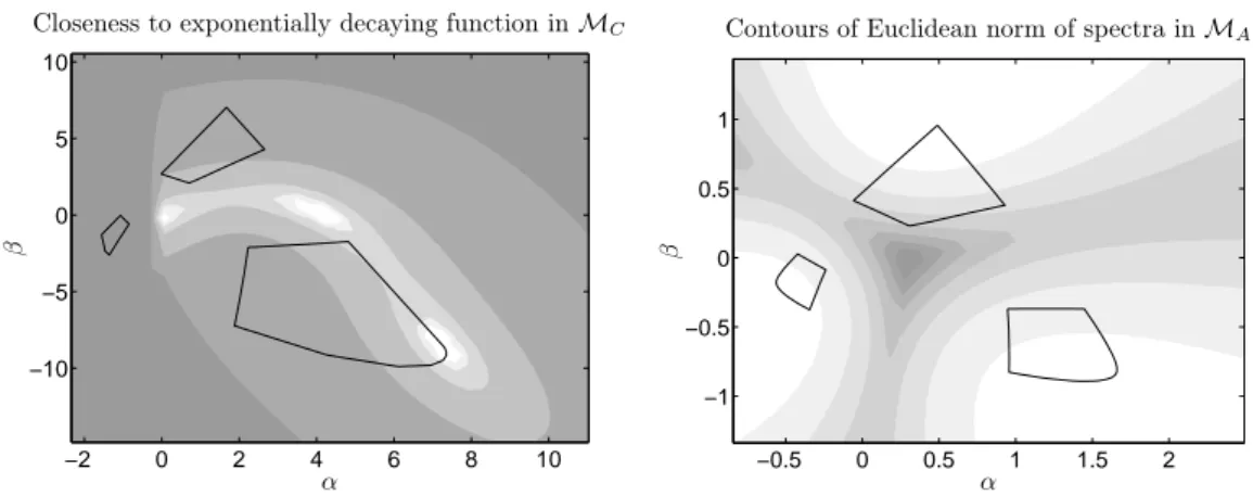
In Figure 5 two contour plots are shown. First, inMA the closeness of a concentration profile to an exponentially decaying function is shown. The smallest distance, which is shown by the lightest grey has the coordinates(α, β)≈(7.2714,−8.5516). This point is the same which is shown in the fourth row and third column of Figure 4 and which can be identified with the reactant X in the model problem from Section 2.1. Second, the contours of the Euclidean norm of the spectra within theMA window.

These contours serve to estimate the total absorbance of the spectra and can for instance be used in order to identify spectra with few and narrow peeaks.

−2 0 2 4 6 8 10

−10

−5 0 5 10

α

β

Closeness to exponentially decaying function inM_C

−0.5 0 0.5 1 1.5 2

−1

−0.5 0 0.5 1

α

β

Contours of Euclidean norm of spectra inM_A

Figure 5: Contour plots within the(α, β)-plane close to the areas of feasible solutionsM_Cand M_A for the data from Section 2.1. Left: Contours of closeness of a concentration profile to an exponentially decaying function in theM_Cwindow. Right: The contour plot of the Euclidean norm (total absorbance) of the pure component spectra within theM_A window.

(8)

3. Users’ guide toFAC-PACK 8

3 Users’ guide to FAC-PACK

Here the users’ guide on the revision 1.1 ofFAC-PACKfollows.

FAC-PACKis an easy-to-use software for the computation of nonnegative multi-component factorizations and for the numerical approximation of the area of feasible solutions (AFS). Revision 1.1 contains new functionalities for the reduction of the rotational ambiguity.

Important features ofFAC-PACKare:

• a fast C program with a graphical user interface (GUI) inMatLab,

• baseline correction of spectral data,

• computation of a low-rank approximation of the spectral data matrix and initial nonnegative matrix factorization,

• computation of the spectral and concentrational AFS by the polygon inflation method,

• applicable to two- and three-component systems,

• live-view mode and factor-locking for a visual exploration of all feasible solutions,

• reduction of the AFS by factor-locking,

• simultaneous representation of the spectral and concentrational AFS,

• reduction of the rotational ambiguity by the complementarity theorem.

3.1 Quick start

Download theFAC-PACKsoftware from

Then extract the software package facpack.zip, open aMatLabdesktop window and start facpack.m.

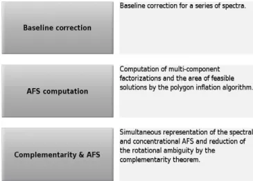
The user can now select one of the three modules ofFAC-PACK, see Figure 6.

3.1.1 Baseline correction module

Step 1: If the baseline needs a correction (e.g., if a background subtraction has partially turned the series of spectra negative), then theBaseline correctionbutton can be pressed. This simple correction method only works for spectral data in which frequency windows with a distorted baseline are clearly separated from the main signal groups of the spectrum; see Figure 7.

Step 2: Load the spectral data matrix. Sample data shown above isexample0.

Step 3: One or more frequency windows should be selected in which more or less only the distorted background signal is present and which are clearly separated from the relevant spectral signals.

In each of these frequency windows (marked blue) the series of spectra is corrected towards zero. However, the correction is applied to the full spectrum. In order to select these frequency windows click the left mouse button within the raw data window, move the mouse pointer and release the mouse button. This procedure can be repeated.

(9)

3.1 Quick start 9

Figure 6: The start window ofFAC-PACK

Step 4: Select the correction method, e.g.polynomial degree 2.

Step 5: Compute the corrected baseline.

Step 6: Save the corrected data.

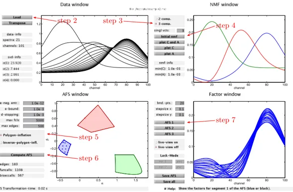
3.1.2 AFS computation module

Step 1: Press the ButtonAFS computationin order to compute the AFS.

Step 2: Selectexample2as sample spectral data matrix.

Step 3: Select3as the number of components.

Step 4: Compute an initial nonnegative matrix factorization (NMF).

Step 5: ChoosePolygon inflation.

Step 6: Compute the AFS which consists of three segments (a blue, red and green segment).

Step 7: Plot the range of spectral factors associated with segment 1 (blue segment) of the AFS.

A second test problem is shown in Figure 9:

Step 1: Selectexample3as the data matrix.

Step 2: Select3as the number of components.

Step 3: Compute an initial nonnegative matrix factorization (NMF).

Step 4: ChooseInverse polygon inflation. The AFS consists of only one segment with a hole.

Step 5: Compute the AFS.

Step 6: Selectlive-view on.

Step 7: Move the mouse pointer through the AFS and watch the interactively computed solutions.

3.1.3 Complementarity & AFS module

Step 1: Press the buttonComplementarity & AFSto activate this GUI.

Step 2: The sample dataexample2can be selected.

Step 3: SelectFIRPOLto plot two supersets including the AFS forC andA and/or selectfullto show

(10)

3.2 Introduction toFAC-PACK 10

0 10 20 30 40 50 60 70 80 90 100

0 0.2 0.4 0.6 0.8 1

channel

0 10 20 30 40 50 60 70 80 90 100

0 0.2 0.4 0.6 0.8 1

channel

step 2

step 3 step 4

step 5

step 6

Figure 7: Baseline correction within 6 steps.

the AFS for the spectral and the AFS for concentrational factor. The sets FIRPOL can easily and quickly be computed; the computation of the AFS forCand forAmay be time-consuming.

Step 4: Click the buttonfirstand move the mouse pointer through the spectral AFS (factorA). A first spectrumA(1,:)can be locked by clicking in the AFS. The associated spectrum is shown in the spectral factor window (right-upper window).

Step 5: Click the buttonsecondand move the mouse pointer once again through the AFS forA. While moving the mouse pointer through the AFS a second spectrumA(2,:)is shown in the spectral factor window together with the unique (by the complementarity theorem) concentration profile of the remaining third component. A certain second spectrumA(2,:)can be locked by clicking in the AFS.

Step 6: Finally, a third spectrum A(3,:) can be selected by moving the mouse pointer through the spectral AFS. The resulting predictions on the spectral factor are shown interactively. This third spectrum can also be locked.

Step 7: These last three buttons and also the buttons first, second, third can be clicked and then a spectrum or concentration profile can be modified by moving the mouse pointer through the AFS. This allows to modify the two triangles in the spectral and concentrational AFS which uniquely determine a feasible factorization of the given spectral data matrix.

In the following sections the functionalities ofFAC-PACKare explained in detail.

3.2 Introduction to FAC-PACK

FAC-PACKis a software for the computation of nonnegative multi-component factorizations and for the numerical approximation of the area of feasible solutions (AFS). Currently, the software can be applied to systems with s= 2ors= 3components.

Given a nonnegative matrixD∈R^k^×ⁿ, which may even be perturbed in a way that some of its entries are slightly negative, a multivariate curve resolution (MCR) technique can be used to find nonnegative matrix factorsC∈R^k^×^sandA∈R^s^×ⁿso that

D≈CA. (1)

Some references on MCR techniques are [10, 8, 12, 11, 15]. Typically the factorization (1) does not

(11)

0 10 20 30 40 50 60 70 80 90 100

0 0.2 0.4 0.6 0.8 1 1.2

channel 00 20 40 60 80 100

0.05 0.1 0.15 0.2 0.25

channel

0 20 40 60 80 100

0 0.05 0.1 0.15 0.2

channel

−0.5 0 0.5 1 1.5

−0.8

−0.6

−0.4

−0.2 0 0.2 0.4 0.6 0.8 1

α

β

step 2 step 3

step 4

step 5

step 6

step 7

Figure 8: Quickstart in 6 steps.

result in unique nonnegative matrix factors C and A. Instead a continuum of possible solutions exists [12, 22, 9]; this non-uniqueness is called the rotational ambiguity of MCR solutions. Sometimes additional information can be used to reduce this rotational ambiguity, see [5, 16] for the use of kinetic models.

The most rigorous approach is to compute the complete continuum of nonnegative matrix factors (C, A) which satisfy (1). In 1985 Borgen and Kowalski [4] found an approach for a low dimensional representation of this continuum of solutions by the so-called area of feasible solutions (AFS). For instance, for a three-component system (s= 3) the AFS is a two-dimensional set. Further references on the AFS are [21, 14, 22, 1]. For a numerical computation of the AFS two methods have been developed: the triangle-boundary-enclosure scheme [6] and the polygon inflation method [18]. FAC- PACKuses the polygon inflation method.

FAC-PACK works as follows: First the data matrix D is loaded. The singular value decomposition (SVD) is used to determine the numbersof independent components underlying the spectral data inD.

FAC-PACKcan be applied to systems withs= 2ors= 3predominating components. Noisy data is not really a problem for the algorithm as far as the SVD is successful in separating the characteristic system data (larger singular values and the associated singular vectors) from the smaller noise-dependent singular values. Then the SVD is used to compute a low rank approximation of D. After this an initial nonnegative matrix factorization (NMF) is computed from the low rank approximation of D.

This NMF is the starting point for the polygon inflation algorithm since it supplies two or three points within the AFS. From these points an initial polygon can be constructed, which is a first coarse approximation of the AFS. The initial polygon is inflated to the AFS by means of an adaptive algorithm. This algorithm allows to compute all three segments of an AFS separately. Sometimes the

(12)

0 10 20 30 40 50 60 70 80 90 100

0 0.2 0.4 0.6 0.8 1

channel 00 20 40 60 80 100

0.05 0.1 0.15 0.2 0.25 0.3 0.35 0.4 0.45 0.5

channel

0 20 40 60 80 100

0 0.05 0.1 0.15 0.2 0.25 0.3 0.35 0.4 0.45 0.5

channel

−0.6 −0.4 −0.2 0 0.2 0.4 0.6 0.8

−0.5 0 0.5 1

α

β

step 1 step 2

step 3

step 4

step 5

step 6 step 7

Figure 9: Quick start withlive-view modein 7 steps.

AFS is a single topologically connected set with a hole. Then an "inverse polygon inflation" scheme is applied. The program allows to compute from the AFS the continuum of admissible spectra. The concentration profiles can be computed if the whole algorithm is applied to the transposed data matrix D^T. Alternatively, the spectral and the concentrational AFS can be computed simultaneously within the “Complementarity & AFS” graphical user interface (GUI).

FAC-PACKprovides a live-view mode which allows an interactive visual inspection of the spectra (or concentration profiles) while moving the mouse pointer through the AFS. Within the live-view mode the user might want to lock a certain point of the AFS, for instance, if a known spectrum has been found. Then a reduced and smaller AFS can be computed, which makes use of the fact that one spectrum is locked. For a three-component system this locking-and-AFS-reduction can be applied to a second point of the AFS.

Within the GUI "Complementarity & AFS" the user can explore the complete factorization D=CA simultaneously in the spectral and the concentrational AFS. The factorizationD=CAis represented by two triangles. The vertices of these triangles can be moved through the AFS and can be locked to appropriate solutions. During this procedure the program always shows the associated concentration profiles and spectra for all components. In this wayFAC-PACKgives the user a complete and visual control on the factorization. It is even possible to import certain pure component spectra or concentration profiles in order to support this selection-and-AFS-reduction process within the "Complementarity

& AFS" GUI.

(13)

3.3 Get ready to start 13

−2 0 2 4 6 8 10

−10

−5 0 5 10

−0.5 0 0.5 1 1.5 2

−1

−0.5 0 0.5 1

0 2 4 6 8 10 12 14 16 18 20

−0.2 0 0.2 0.4 0.6 0.8 1

0 10 20 30 40 50 60 70 80 90 100

−0.2 0 0.2 0.4 0.6 0.8

step 2 1

step 3

step 5 step 4

step 6 step 7

Figure 10: The complementarity & AFS module.

3.3 Get ready to start

Please download FAC-PACKfrom

Then extract the file facpack.zip. Open aMatLabdesktop and runfacpack.m.

This software is shareware that can be used by private and scientific users. In all other cases (e.g. com- mercial use) please contact the authors. We cannot guarantee that the software is free of errors and that it can successfully be used for a particular purpose.

3.3.1 Program structure

The current revision ofFAC-PACKconsists of three graphical user interface (GUI) windows to solve the following problems in multivariate curve resolution:

1. Correction of the baseline for given spectroscopic data or pre-processed data, e.g., after background subtraction,

2. Computation of the area of feasible solutions for two- and three-component systems,

3. Simultaneous representation of the spectral and concentrational AFS and interactive reduction of the rotational ambiguity up to uniqueness by means of the complementarity theorem [17, 20].

OnceFAC-PACKis started it is necessary to select one of the three GUIs "Baseline correction", "AFS computation" or "Complementarity & AFS". No additional MatLab toolboxes are required to run the software.

Baseline correction This GUI has the following two windows:

(14)

3.3 Get ready to start 14

1. Raw data window (Left window): The raw data window shows thek raw spectra which are the rows of the data matrixD∈R^k×n.

2. Baseline corrected data window (Right window): This window shows the control parameters for the baseline computation together with the corrected spectra. Seven simple functions (polynomials, Gaussian- and Lorentz curves) can be used to approximate the baseline.

AFS computation The GUI uses four windows:

1. Data window (Upper-left window): The data window shows the k rows (spectra) of the data matrixD∈R^k×nin a 2D-plot. The number of spectrakis printed together with the number of spectral channelsn. The four largest singular values ofD are shown. By transposing the data matrixDit is possible to compute the AFS for the concentration factorC (instead of the AFS for the spectral factorA).

2. NMF window (Upper-right window): This window allows to set the number of components to s= 2ors= 3and to compute an initial NMF. The smallest minimal components ofC andA are printed. The figure shows the profiles of the so-called abstract matrix factors. The buttons allow to compute the profiles ofCand/orA.

3. AFS window (Lower-left window): Various control parameters allow to make certain settings for the AFS computation in order to control the approximation quality or maximal number of edges.

Pressing theCompute AFSbutton starts the AFS computation. The live-view mode is active after the AFS has been drawn. Just move the mouse pointer to (and through) the AFS.

4. Factor window (Lower-right window): This window shows the spectral factors (or concentration profiles if the transpose option has been activated in the first window) for the grid points shown in the AFS window.

Complementarity & AFS The GUI is built around four windows and a central control bar:

1. Pure factor windows (Upper row): These windows show three concentration profiles and three spectra of a factorizationD=CAwhich is computed by a step-wise reduction of the rotational ambiguity for a three-component system.

2. C,A- AFS windows (Lower row): Here FIRPOL, a superset which includes the AFS, and/or the AFS can be shown for the factorsC andA. A feasible factorization D =CAis associated with two triangles whose vertices represent the concentration profiles and spectra.

3. Control bar (Center): Includes all control parameters for the computations, the live-view mode, the import of pure component spectra or concentration profiles as well as the control buttons for adding contour plots on certain soft constraints.

3.3.2 Importing initial data

Spectral data are imported to FAC-PACK by means of a MAT-file ∗.mat. This file must contain the matrix D ∈ R^k×n whose rows are the k spectra. Each spectrum contains absorption values at n frequencies. The file may also contain a vector x with n components representing the spectral wavenumbers/frequencies and a time-coordinates vectort∈R^k.

The spectral data matrix Dis loaded by pressing one of the buttons (1)¹, (18) or (64) depending on the active GUI. The dimension parametersk andn are shown in the GUI. The four largest singular values are shown in the fields (22)-(25) or (71)-(74). These singular values allow to determine the numerical rank of the data matrix and are the basis for assigning the number of componentss.

1Red numbers refer to Section 3.7.

(15)

3.4 Baseline correction module 15

3.3.3 Sample data

FAC-PACKprovides some sample data matrices:

example0.mat: k= 51spectra,n= 201channels,s= 3components with a baseline turning negative to demonstrate the baseline correction.

example1.mat: k= 51spectra,n= 101channels,s= 2components.

example2.mat: k= 21spectra,n= 101channels,s= 3components, the AFS has three clearly separated segments.

example3.mat: k= 21spectra,n= 101channels,s= 3components, the AFS is one topologically connected set with a hole.

example4.mat: some random noise has been added to data matrixD given in example2.mat, the AFS has three clearly separated segments.

3.3.4 External C-routine

All time-consuming numerical computations are externalized to a C-routine in order to accelerate FAC-PACK. This C-routine is AFScomputationSYSTEMNAME.exe, wherein SYSTEMNAME stands for your system including the bit-version. For example AFScomputationWINDOWS64.exeis used on a 64 bit Windows system. The external routine is called if any of the buttons Initial nmf (30), Compute AFS(43),no. 1(57) orno. 2(59) is pressed. Pre-compiled versions of theC-routine for the following systems are parts of the distribution:

- Windows 32/64 bit, - Unix 32/64 bit and - Mac 64 bit.

The execution of the external routine can always be stopped byCTRL + Cin the command window.

If the C-routine takes too much computation time, the reason for this can be large values fork,n,max fcls(40) ormax edges(41) or too small values forε-bound(38) orδ-stopping(39).

3.3.5 Further included libraries

The C-routineAFScomputationSYSTEMNAME.exeincludes thenetliblibrarylapackand theACMrou- tinenl2sol. Any use ofFAC-PACKmust respect

thelapacklicense, seehttp://www.netlib.org/lapack/LICENSE.txt, and

thenl2sollicense, seehttp://www.acm.org/publications/policies/softwarecrnotice.

3.4 Baseline correction module

AFS computations depend sensitively on distorted baselines and negative components in the spectral data. Such perturbing signals can pretend further components in the reaction system and negative components are not consistent with the nonnegative factorization problem. TheBaseline correction GUI tries to correct the baseline and is accessible by pressing the buttonBaseline correctionon the FAC-PACK start window, see a screen shot on page 32. Data loading is explained in Section 3.3.2.

TheTransposebutton (2) serves to transpose the data matrixD.

TheBaseline correctionGUI is a simple tool for spectral data preprocessing. It can be applied to series of spectra in which the distorted baseline in some frequency windows is well separated from the relevant signal. We call such frequency intervals, which more or less show the baseline, zero-intervals.

(16)

3.4 Baseline correction module 16

The idea is to remove the disturbing baseline from the series of spectra by adapting a global correction function within in the zero-intervals to the baseline. See Figure 11 where four zero-intervals have been marked by blue columns. The zero-intervals are selected in the raw data window (8) by clicking in the window, dragging a blue zero-interval and releasing the mouse button. The procedure can be repeated in order to define multiple zero-intervals. The Reset intervals button (7) can be used in order to reset the selection of all zero-intervals.

0 20 40 60 80 100

0 0.2 0.4 0.6 0.8 1

channel

Raw spectra

Figure 11: Four zero-intervals are marked by blue columns. In these intervals the spectral data is corrected towards zero. Data: example0.mat.

Mathematically every spectrum is treated separately. Let a∈ Rⁿ be a certain spectrum. Then the aim is to compute a baseline functionb∈Rⁿso that the norm of the residuuma−bis minimal within the selected intervals. The baseline-corrected spectrum is thenanew=a−b. Once again, this explains the naming zero-intervals, since there the spectrum is assumed to be zero.

The sum of the interval lengths of these zero-intervals should be as large as possible in order to ensure a reliable baseline approximation. However, the required number of frequency grid points depends on the degrees of freedom of the type of the baseline function. The text field (11) shows the information

"ok"/"not ok" in order to indicate whether or not the selected intervals are large enough for the baseline approximation. Data cutting is a further functionality of the baseline correction GUI: If only a certain frequency subinterval is to be analyzed or the baseline correction is only to be applied to a subinterval, then this subinterval can be marked by mouse clicking and dragging and then the Cut data-button can be pressed. The user can always return to the initial data by pressing theReset cutting-button (6).

3.4.1 Type of the baseline Four types of baselines are available:

• Polynomials of order zero up to order four,

• a Gauss curve,

• or a Lorentz curve.

The most recommended baselines are polynomials with the degrees 0, 1 or 2. A polynomial of degree 0 is a constant function so that a constant is added or subtracted for each spectral channel of a spectrum.

(17)

3.5 AFS computation module 17

The baselines "Gauss curve" and "Lorentz curve" can be used to remove single isolated peaks from the series of spectra. Once again, the curve profile is fitted in the least-squares sense to the spectroscopic data within the selected frequency interval. Then the fitted profile is subtracted from the spectrum.

3.4.2 Program execution and data export

The baseline correction by an external C-procedure is started by pressing theCorrect baseline-button (12). The computation times for data wrapping and for solving the least-squares problem are shown in the text fields (13) and (14). The corrected series of spectra (in black) is shown in the window (16) together with the original data (in gray). The baseline-corrected data can be stored in aMatLabfile by pressing theSave-button (15).

By clicking the right mouse button in a figure a separateMatLab figure opens. The figure can now be modified, printed or exported in the usual way. If for some reason (e.g. program runs too long) the external C-procedure for the baseline correction is to be stopped, thenCTRL + Conly works the MatLab command window (and not in the GUI).

0 20 40 60 80 100

0 0.2 0.4 0.6 0.8 1

channel

Baseline corrected series of spectra

Figure 12: Sample problemexample0.matwith corrected baseline by a 2nd order polynomial.

3.5 AFS computation module

This section describes how to compute the area of feasible solutions (AFS) for two- and three- component systems withFAC-PACK.

3.5.1 Initial steps

The AFS computation module can be started by pressing theAFS computationbutton on theFAC- PACKstart window. Data loading by theLoadbutton (18) is explained in Section 3.3.2. The loading process is followed by a singular value decomposition (SVD) of the data matrix. The computing time is printed in the fieldComputing time info(47). The dimensions ofDare shown in the data window together with the singular valuesσ1, . . . , σ4. These singular values allow to determine the "numerical rank" of the data matrix and are the basis for assigning the number of components s in the NMF window.

(18)

FAC-PACK provides some sample data matrices. These sample data sets are introduced in Section 3.3.3. Figure 13 shows the series of spectra from example2.mat. Three clearly nonnegative singular values indicate a three-component system.

3.5.2 Transposing the problem

FAC-PACK computes and displays the spectral matrix factor A, see (1), together with its AFS. In order to compute the first matrix factorCand its AFS, press theTransposebutton (19) to transpose the matrixD and to interchangexandt.

3.5.3 Initial NMF

To run the polygon inflation algorithm an initial NMF is required. First the number of components (eithers= 2ors= 3) is to be assigned. In the case of noisy data additional singular vectors can be used for the decomposition by selecting a larger number ofsingl vcts(29). For details on this option see [13], wherein the variablez equalssingl vcts.

The initial NMF is computed by pressing the button Initial nmf (30). The NMF uses a genetic algorithm and a least-squares minimizer. The smallest relative entries in the columns ofCand rows of A, see [18] for the normalization of the columns ofCand rows ofA, are also shown in the NMF window, see (34) and (35). These quantities are used to define an appropriate noise-levelε; see Equation (6) in [18] for details.

The initial NMF provides a number of sinterior points of the AFS; see Equations (3) and (5) in [18].

The buttonsplot C and A(31),plot C(32) andplot A(33) serve to display the factorsC andA together or separately. Note that these abstract factors are associated with the current NMF. After an NMF computation theAfactor is displayed.

Figure 14 shows the factorAfor an NMF forexample2.mat. The relative minimal components in both factors are greater than zero (9.9·10⁻⁴ and10⁻³). So the noise-levele-neg. entr.: (37) can be set to the lower bounde-neg. entr.: 1·10⁻¹².

3.5.4 Computation of the AFS

For two-component systems (s= 2) the AFS consists of two real intervals. FAC-PACKrepresents the associated AFS by the two orthogonal sides of a rectangle. The sides are just the intervals of admissible values forαandβwhere

T =

1 α 1 β

is the transformation matrix which constitutes the rotational ambiguity. See [1, 2] for the AFS for the cases= 2. However in [1], see Equation (6), the entries of the second row ofT are interchanged.

For three-component systems (s= 3) the AFS is formed by all points(α, β)so that

T =





1 α β

1 s11 s12

1 s21 s22





is a transformation which is associated with nonnegative factors C and A, see [18]. A permutation argument shows that with(α, β)the points(s11, s12)and(s21, s22)belong to the AFS, too.

(19)

0 10 20 30 40 50 60 70 80 90 100

0 0.2 0.4 0.6 0.8 1 1.2

channel

Figure 13: Test matrixexample2.matloaded by pressing theLoadbutton (18).

0 20 40 60 80 100

0 0.05 0.1 0.15 0.2 0.25

channel

Figure 14: The initial NMF forexample2.matwith s= 3components.

(20)

The initial NMF is the starting point for the numerical computation of the AFS since it provides first αandβin the AFS.

Next various control parameters for the numerical computation of the AFS are explained. Further two ways of computing different kinds of the AFS are introduced.

Control parameters Five control parameters are used to steer the adaptive polygon inflation algorithm. FAC-PACKaims at the best possible approximation of the AFS with the smallest computational costs. Default values are pre-given for these control parameters.

• The parametere-neg. entr. (37) is the noise level control parameter which is denoted byεin [18]. Negative matrix elements ofCandAdo not contribute to the penalization functional if their relative magnitude is larger than−ε. In other words, an NMF with such slightly nonnegative matrix elements is accepted as valid.

• The parametere-bound(38) controls the precision of the boundary approximation and is denoted by εb in [18]. Decreasing the value εb improves the accuracy of the positioning of new vertices of the polygon.

• The parameterd-stopping(39) controls the termination of the adaptive polygon inflation procedure. This parameter is denoted byδin Section 3.5 of [18] and is an upper bound for change- of-area which can be gained by a further subdivision of any of the edges of the polygon.

• max fcls. (40) andmax edges(41) are upper bounds for the number of function-calls and for the number of vertices of the polygon.

Type of polygon inflation FAC-PACKoffers two possibilities to apply the polygon inflation method for systems with three components (s= 3). The user should select the proper method according to the following explanations:

1. The "classical" version of the polygon inflation algorithm is introduced in [18] and applies best to an AFS which consists of three clearly separated segments. Select Polygon inflation by pressing the upper button (42). A typical example is shown in Figure 15 for the test problem example2.mat. In each of the segments an initial polygon has been inflated from the interior.

Interior points are accessible from an initial NMF.

2. Alternatively, the Inverse polygon inflation procedure is activated by pressing the lower button in (42). This should be done if the AFS is only one topologically connected set (with a hole) or if the isolated segments of AFS are in close neighborhood. See Figure 16 for an example.

The inverse polygon inflation method is more expensive than the classical version. First the complement of the AFS is computed and then some superset of the AFS is computed. A set subtraction results in the desired AFS. The details are explained in [20].

The user should always try the second variant of the polygon inflation algorithm if the results of the first variant are not satisfying or if something appears to be doubtful.

3.5.5 Factor representation & live-view mode

Next the plotting of the spectra and/or concentration profiles is described. These factors can be computed from the AFS by certain linear combinations of the right and/or left singular vectors. The live-view mode allows an interactive representation of the factors by moving the mouse pointer through the AFS.

(21)

−0.5 0 0.5 1 1.5

−0.8

−0.6

−0.4

−0.2 0 0.2 0.4 0.6 0.8 1

α

β

Figure 15: An AFS with three clearly separated segments as computed by the "classical"

polygon inflation algorithm. Data: example2.mat.

−0.6 −0.4 −0.2 0 0.2 0.4 0.6 0.8

−0.5 0 0.5 1

α

β

Figure 16: An AFS which consists of only one segment with a hole. For the computation the inverse polygon inflation algorithm has been applied toexample3.mat.

(22)

0 20 40 60 80 100

0

channel / time

Figure 17: The live-view mode for the two-component system example1.mat. By moving the mouse pointer through the AFS the transformation to the factorsCand Ais computed interactively and all results are plotted in the factor window. The spectra are drawn by solid lines and the concentration profiles are represented by dash-dotted lines.

−0.5 0 0.5 1 1.5

−0.5 0 0.5 1

α

β

AFS

0 20 40 60 80 100

0 0.05 0.1 0.15 0.2

channel Solution

Figure 18: The AFS for the problemexample2.matconsists of three separated segments. The blue segment of the AFS is covered with grid points (dark blue points). For each of these points the associated spectrum is plotted in the right figure.

−0.5 0 0.5 1 1.5

−0.5 0 0.5 1

α

β

AFS

0 20 40 60 80 100

0 0.1 0.2 0.3 0.4

channel Solution

(x,y) = (0.9896, −0.4196)

Figure 19: The live-view mode is active for the 3 component system example2.mat. In the green AFS-segment the mouse pointer is positioned in the left upper corner at the coordinates(0.9896,−0.4196). The associated spectrum is shown in the right figure together with the mouse pointer coordinates.

(23)

Two-component systems For two-component systems a full and simultaneous representation of the factors C and A is possible. In order to get an overview of the range of possible spectra one can discretize the AFS-intervals equidistantly. For each point of the resulting 2D discrete grid the associated spectrum is plotted in the factor window. The discretization parameter (subinterval length) is selected in the field (50) and/or (51). The plot of the spectra is activated by pressing buttonAFS 1(52) or buttonAFS 2(53).

Live-view mode: The live-view mode can be activated in the field (55). By moving the pointer through the AFS the associated solutions are shown interactively. Figure 17 shows a typical screen shot. The y-axis labels are turned off.

Three component systems For three-component systems the range of possible solutions is presented for each segment of the AFS separately. The user can select with the buttons AFS 1 (52), AFS 2(53) andAFS 3(54) a specific AFS which is then covered by a grid. First the boundary of the AFS segment (which is a closed curve) is discretized by a number ofbnd-ptsnodes. The discretization parameters for the interior of this AFS segment arestep size x(50) andstep size y(51); the interior points are constructed line by line. The resulting nodes are shown in the AFS window by symbols

×in the color of the AFS segment. For each of these nodes the associated spectrum is drawn in the factor window. For the test problemexample2.matthe bundle of spectra is shown in Figure 18. The resolution can be refined by increasing the number of points on the boundary or by decreasing the step size in the direction ofxory.

If the admissible concentration profiles are to be printed, then the whole procedure is to be applied to the transposed data matrix D; activate the Transposebutton (19) at the beginning and recompute everything.

Live-view mode: The live-view mode can be activated in the field (55). By moving the pointer through the AFS, the associated solutions are shown interactively. An example is shown in Figure 19.

Additionally, a certain point in the AFS can be locked by clicking the left mouse button; then the AFS for the remaining two components is re-computed. The resulting AFS is a smaller subset of the original AFS, which reflects the fact that some additional information is added by locking a certain point of the AFS. See Section 3.5.6 for further explanations.

3.5.6 Reduction of the rotational ambiguity

With the computation of the AFS FAC-PACKprovides a continuum of admissible matrix factorizations. All these factorizations are mathematically correct in the sense that they represent nonnegative matrix factors, whose product reproduces the original data matrixD. However, the user aims at the one solution which is believed to represent the chemical system correctly. Additional information on the system can help to reduce the so-called rotational ambiguity. FAC-PACKsupports the user in this way. If, for instance one spectrum within the continuum of possible spectra is detected, which can be associated with a known chemical compound, then this spectrum can be locked and the resulting restrictions can be used to reduce the AFS for the remaining components.

Locking a first spectrum After computing the AFS, activate the live-viewmode (55). While moving the mouse pointer through any segment of the AFS, the factor window shows the associated spectra. If a certain (known) spectrum is found, then the user can lock this spectrum by clicking the left mouse button. A×is plotted into the AFS and the buttonno. 1(56) becomes active. By pressing this button a smaller subset of the original AFS is drawn by solid black lines in the AFS window. This

(24)

−0.5 0 0.5 1 1.5

−0.5 0 0.5 1

α

β

AFS

−0.5 0 0.5 1 1.5

−0.5 0 0.5 1

α

β

AFS

Figure 20: Reduction of the AFS for the test problem example2.mat. Left: the reduced AFS is shown by black solid lines after locking a first spectrum (marker×). Right: The AFS of the remaining third component is shown by a black broken line.

smaller AFS reflects the fact that some additional information on the system has been added. The buttonesc(57) can be used for unlocking any previously locked point.

Locking a second spectrum Having locked a first spectrum and having computed the reduced AFS the live-viewmode can be reactivated. Then a second point within the reduced AFS can be locked. By pressing buttonno. 2(58) the AFS for the remaining component is reduced for a second time and is shown as a black broken line. Once again, the buttonesc(59) can be used for unlocking the second point.

Figure 20 shows the result of such a locking-and-AFS-reduction procedure for the test problemexam- ple2.mat. For this problem the AFS consists of three clearly separated segments and the final reduction of the AFS is shown by the black broken line in the red segment of the AFS. The live-view mode allows to display the possible spectra along this line. The resulting restrictions on the complementary concentration factorC can be computed by the module AFS & Complementarity, see Section 3.6.

3.5.7 Save data and extract axes

To save the results in aMatLab *.mat file press eitherSave AFS(60) orSave all(61). A proper file name is suggested.

Save AFS saves the data D, the factors U, S, V of the singular value decomposition, the factors Cinit, Ainit of the initial NMF and the AFS. The AFS has the data format of a structure which contains the following variables:

• For s = 2 the AFS consists of two segments: AF S{1} ∈ R² and AF S{2} ∈ R² with α ∈ [AF S{1}(1), AF S{1}(2)] andβ∈[AF S{2}(1), AF S{2}(2)]and vice versa.

• For s = 3 and an AFS consisting of three segments: AF S{i} ∈ R^mⁱ^×2 with i = 1,2,3 is a polygon whosex-coordinates areAF S{i}(:,1)and whosey-coordinates areAF S{i}(:,2).

• For s = 3 and an AFS consisting of one segment with a hole: AF S{1} ∈ R^m×2 is the outer polygon (AF S{1}(:,1) thex-coordinates and AF S{1}(:,2)the y-coordinates) andAF S{2} ∈

(25)

3.6 Complementarity & AFS module 25

R^ℓ^×2 is the inner polygon surrounding the hole.

If the lock-mode has been used, see Section 3.5.6, then the results are saved inAF SLockM ode1and LockP oint2 (case of one locked spectrum) as well asAF SLockM ode2and LockP oint1(case of two locked spectra).

The user can get access to all figures. Therefore click the right mouse button in the desired figure.

Then a separate MatLabfigure opens. The figure can now be modified, printed or exported in the usual way.

3.5.8 Cancellation of the program

Whenever the buttonsInitial nmf(30),Compute AFS(43),no. 1(57) orno. 2(59) are pressed, an external C-routine is called, see Section 3.3.4. The GUI does not respond to any activities during the execution of the C-routine. Therefore, in case of any problems or in case of too long program runtimes, the C-routine cannot be canceled from the GUI. The termination can be enforced by typing CTRL + C in the MatLab command window. Time consuming processes can be avoided if all the parameters are adjusted to reasonable (default) values.

3.5.9 How to get help

If theHelpbox (62) is checked and the mouse pointer is moved over a button, a text field or an axis, then a short explanation appears right next to theHelpfield. Further, a small pop-up window opens if the mouse pointer rests for more than one second on a button.

3.6 Complementarity & AFS module

This FAC-PACKmodule simultaneously shows the AFS for the spectral factor and the AFS for the concentration factor. It demonstrates how the rotational ambiguity for a three-component system can be reduced by means of the complementarity theory. For the complementarity theorem see [19, 20]

and for comparable results see [3]. Solutions can be selected and modified within a live-view mode.

Any changes in the spectral AFS are immediately mapped to changes in the concentrational AFS and vice versa. This gives the user the full control over and a visualization of a the complete factorization D=CA.

3.6.1 Initial steps

The Complementarity & AFS module module can be started by pressing theComplementarity &

AFSbutton on theFAC-PACKstart window. Data loading by theLoadbutton (18) is explained in Section 3.3.2. The loading process is followed by a singular value decomposition (SVD) of the data matrix. The dimensions of D are shown in the fields (69) and (70) together with the four largest singular values in the fields (71-74). For this module the fourth singular value should be "small"

compared to the first three singular values so that the numerical rank of D equals 3. For noisy data one might try to use a larger number of vectors in the field (78), see also Section 3.5.3.

In Figure 13 we consider the sample dataexample2.mat, cf. Section 3.3.3. The parameters in the fields (75)-(77) control the AFS computation. The meaning of these parameters is explained in Section 3.5.4.